



Abstract
We estimate intraday periodicities in return volatility by implementing two time series procedures—flexible Fourier form and cubic spline. We use intraday data for more than five years for crude oil futures contracts traded at the Multi Commodity Exchange India Limited. Filtration of the intraday periodicities from the raw returns reveals long-run dependence in volatility. We observe the presence of recurring and consistent intraday patterns in return volatility. Further, we find that adjustment for the intraday periodicity in return volatility improves forecasting performance. Our results are robust after controlling for the scheduled macroeconomic announcements.
Introduction
Existence of consistent and recurring intraday patterns in return volatility across global markets and financial instruments has been widely documented in finance literature, particularly, U-shaped patterns in volatility during the trading day has attracted a great deal of attention from researchers (for example, see Abhyankar, Ghosh, Levin, & Limmack, 1997; Cai, Hudson, R., & Keasey, 2004; Daigler, 1997; Ekman, 1992; Harris, 1986; Wood, McInish, & Ord, 1985). Andersen and Bollerslev (1997) showed that the presence of intraday periodic patterns induce distortions in volatility estimation process. Therefore, volatility prediction without adjusting intraday periodicity may be misleading. The number of higher observations in high frequency data than daily data, compared to the identifiable shocks, potentially provides a more accurate forecast of return volatility (McMillan & Speight, 2004).
Time series procedures— Fourier flexible form (FFF) and cubic spline are very successful in estimating intraday periodicities in return volatility (Andersen, Bollerslev & Cai, 2000; McMillan & Speight, 2010). Andersen and Bollerslev (1997) suggest a sequential estimation or ‘two-step procedure’ for the adjustment of intraday periodicities in volatility modelling. In the first step—we obtain filtered returns by removing the deterministic periodicity components from the raw returns and then in the second step—volatility models are applied on the filtered returns. Cai et al. (2000) use the FFF to estimate the intraday periodicities for gold futures contracts traded at COMEX, a division of NYMEX. They conclude that an adjustment for the intraday periodicities is necessary to study the characteristics of intraday volatility. Andersen, Bollerslev and Cai (2000) and Bollerslev, Cai and Song (2000) find long memory dependence after the filtration of intraday periodicities in return volatility for the Nikkei 225 index and US Treasury bond futures.
Engle and Russell (1998) implement the cubic spline approach to estimate the time-adjusted duration in autoregressive conditional duration (ACD) models for irregularly spaced tick data. This approach fits three-degree polynomials between the pre-specified knots fixed at the points where changes in intraday patterns are expected. Taylor (2004b) and Giot (2005) implement the cubic spline approach in an ACD framework for the FTSE-100 index futures and stocks traded on the NYSE. Evans and Speight (2010) applied both FFF and cubic spline approaches to study the effect of calendar and macroeconomic announcements on intraday periodicities for Euro-Dollar, Euro-Sterling, and Euro-Yen exchange rates. They find that calendar and macroeconomic announcements have an impact of intraday periodicities. However, they do not find any economic significance from those announcements.
The characteristics of intraday periodicities in return volatility and accurate volatility forecasting are very useful for market participants such as day traders, algorithmic traders, high-frequency portfolio managers, scalpers, and hedgers, since they need to evaluate the risk involved in their portfolios more frequently than long-term investors. This study provides an extensive analysis of intraday patterns in return volatility for crude oil futures contracts, which is the most liquid futures contract traded at the Multi Commodity Exchange of India Ltd (MCX). During the year 2010, approximately 78,257 contracts were traded daily. We used 10-minute interval data spanning more than five years from June 2005 to December 2010. Studies on Indian commodity futures market are rare, although it is a one of the fastest-growing emerging markets. Since the inception of the national commodity exchanges in 2003, the commodity futures market in India has witnessed a rapid growth in volume. Trading volume (in terms of value of trade) in all the exchanges during 2010–11 was approximately US$2.5 trillion. Details about the commodity contracts trading in Indian market has been provided in Table 1. Within six years of its inception, the MCX became the fourth largest derivatives exchange in Asia. According to the 2010 Volume Survey Report 2010 of Futures Industry Association, Washington, US, the MCX is the sixth largest commodities exchange in the world in terms of the number of traded contracts during April 2009 to March 2010.
This study extends the extant finance literature in many ways. First, it analyses oil futures contracts traded in the Indian commodity market which is an emerging market and is unexplored in this econometric framework. Second, the extensive analysis of intraday periodicity in return volatility is mainly limited to foreign exchange rate markets and market indices. Commodity futures markets are still unexplored though it is required to test the robustness of the results obtained in other markets. Third, we employed two alternative techniques—FFF and cubic spline, to capture and test the importance of intraday periodicities in volatility modelling.
We find the presence of intraday periodicities in the return volatility. Our results suggest that the filtration of deterministic intraday periodicities reveals long-run dependence property in volatility. Our findings suggest that an adjustment for the intraday periodicity in return volatility results in improved volatility estimates and volatility forecasting.
The remainder of this paper is structured as follows: Section 2 describes the data and provides statistical analysis of intraday periodicity and the correlation structure of intraday returns and volatility. Section 3 discusses the methodology for estimating and the adjustment procedure for intraday periodicities in the volatility model. Estimates of intraday periodicities and volatility forecast are discussed in Section 4 and finally, Section 5 concludes the study.
Most Liquid Commodities Traded in National Exchanges
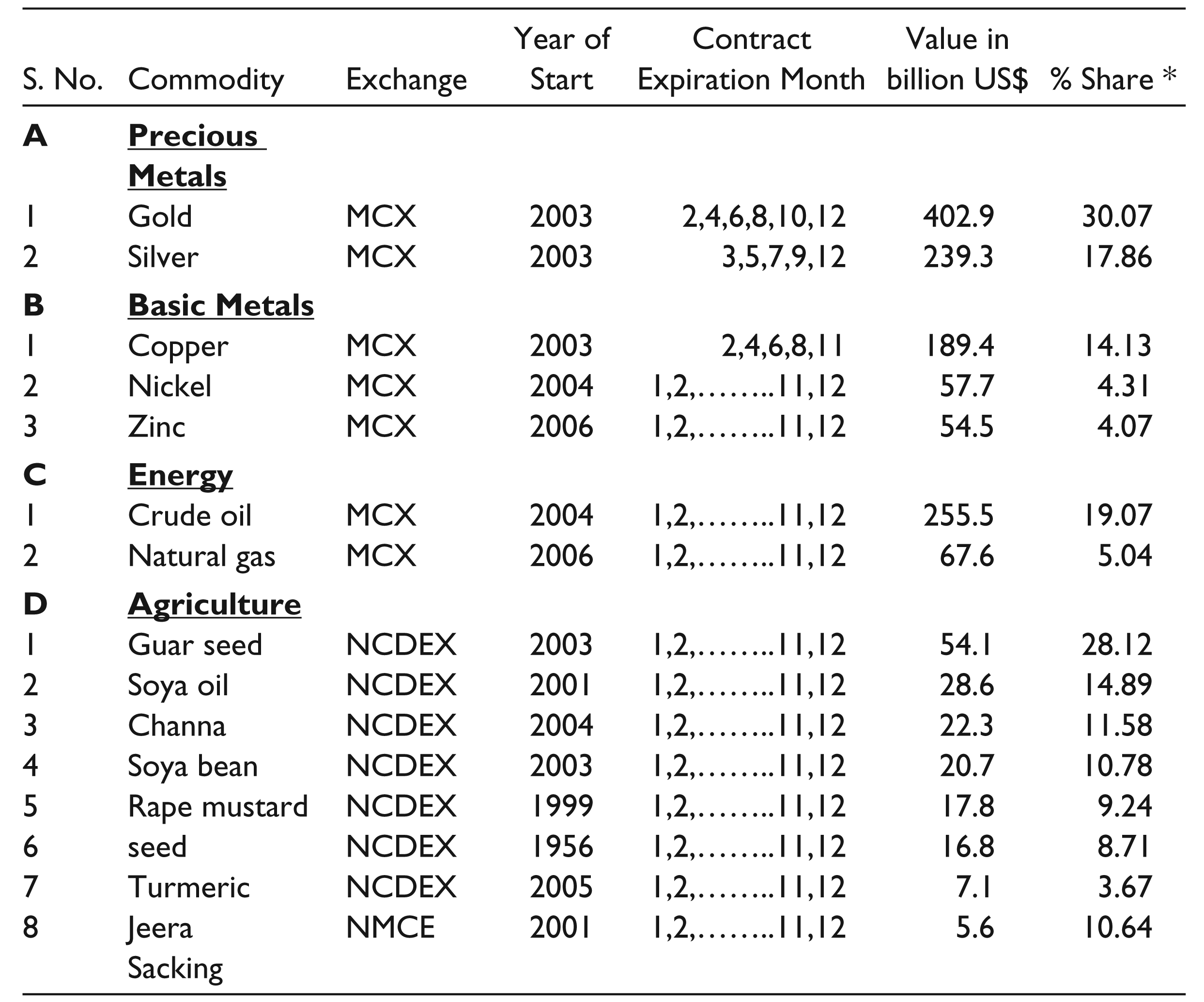
Most Liquid Commodities Traded in National Exchanges
We obtained intraday proprietary data at 10-minute intervals for the nearest to maturity months, from the exchange for crude oil futures contracts from June 2005 to December 2010, which provides data of 1,375 days for 65 contracts. The data are composed of the best bid price/quantity, best ask price/quantity, open and the last traded price for each time interval for the nearest month to expiration contracts.
The Press Information Bureau, India, provides data for macro-economic announcements with the time stamp near to minute. The data set covers press releases about the estimates of the monthly industrial production index, monthly export and import, the weekly wholesale price index, monthly oil and natural gas production, and announcements of Bond and T-bill auctions. They also report on actions taken by the central bank related to the monetary policy such as change in repo rates, reverse repo rate, bank rates, etc.
MCX provides a trading window from 10:00

Rt,n is the return for nth 10-minute interval on the day t, t= 1, 2, … T. T denotes the trading days and n=1, 2, … N denotes the number of intervals during the day t.
Descriptive statistics for the 10-minute returns show that returns are not different from zero (–0.0000171). Ten-minute returns show the presence of fat tails and high peak as the skewness comes to be –0.348 and kurtosis 18.731. Jarque-Bera statistics show that the returns are not normal.
Identification of Intraday Periodicities
In order to identify the intraday patterns in return volatility, we draw (Figure 1) the average of 10-minute returns and absolute returns across all intervals. We use absolute return as the proxy for return volatility. Pagan and Schwert (1990) among others, pointed out that absolute return reduces the influence of heavy tails and occasional shocks, which is in accordance with the literature (e.g., see Evans & Speight, 2010). 1

Return volatility is high at the opening then it declines sharply and again starts rising around 1:00
Further, to characterize intraday periodicity in return volatility, we plotted a day-correlogram, which is shown in Figure 2.
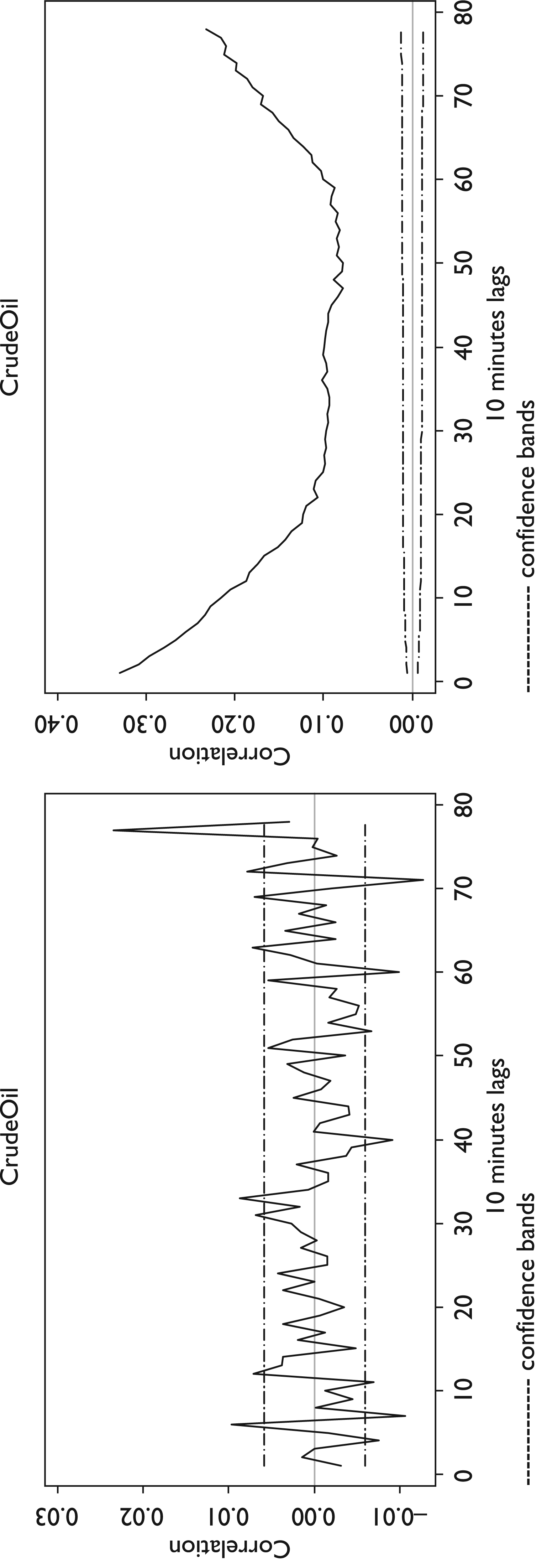
The correlogram for 10-minute returns (left panels) in Figure 2 does not show any discernible patterns and violates the 95% confidence interval band at several lags, but it does not suggest any particular order for the return process. The day-correlogram for return volatility (right panel) shows a spike at first lag, declines sharply for higher lags and again starts rising until the end creating a distorted U shape. If these patterns are consistent across all the days, it may cause distortion in the long-run persistence of return volatility.
Several studies such as Poshakwale (1996), Murry and Zhu (2004), and Nath and Dalvi (2005) find a day-of-the-week effect in returns and return volatility. To be more conclusive and to capture the day-of-the-week effect, we plotted a 5-day correlogram.
Five-day Correlogram for 10-minute Absolute Returns
Figure 3 shows a correlogram for weekdays, that is, from Monday to Friday. The autocorrelation patterns in the correlogram show the presence of cyclical patterns in return volatility indicating the presence of deterministic intraday patterns in return volatility. The 5-day correlogram shows a small rise instead of decay in autocorrelations for Fridays. An increase in autocorrelations on Friday indicates the presence of a day-of-the-week effect. These results confirm the patterns observed in previous studies on foreign exchange markets (e.g., Andersen & Bollerslev, 1997, 1998; Bollerslev et al., 2000; Andersen et al., 2000).

Modeling Intraday Periodicity
From earlier studies by Wood et al. (1985), Ekman (1992) and Daigler (1997), periodicity in return, volatility is estimated as the average of return volatility across the trading days. In this study, we estimate intraday periodicity in return volatility by using two time series approaches—FFF and cubic spline. The advantage of the time series procedures such as FFF and cubic spline is that they use complete time series data in estimating the desired model and provides estimates that are more reliable.
Flexible Fourier Form
Andersen and Bollerslev (1998) pointed out that the volatility process can be assumed to be driven by the calendar effect, macroeconomic news announcement effect and volatility persistent factor. Intraday returns can be decomposed as

where Rt,n is the intraday return for the nth interval on day t. is the price of the asset at the end of nth interval on day t. E(Rt,n) denotes the expected return of nth interval on day t. N is the number of time intervals per day. σt,n is the remaining long memory volatility component for the nth interval on day t. St,n denotes the intraday periodicity component which includes the calendar effect and macroeconomic announcement effects observed during the nth interval on day t. Zt,n is an i.i.d error term with a mean of zero and unit variance that is assumed to be independent from the daily volatility process.
The components of equation (1) are not separately identifiable. Using the logarithm and rearranging the terms, we get

E(Rt,n) may be approximated with the average of intraday returns across trading days, whereas
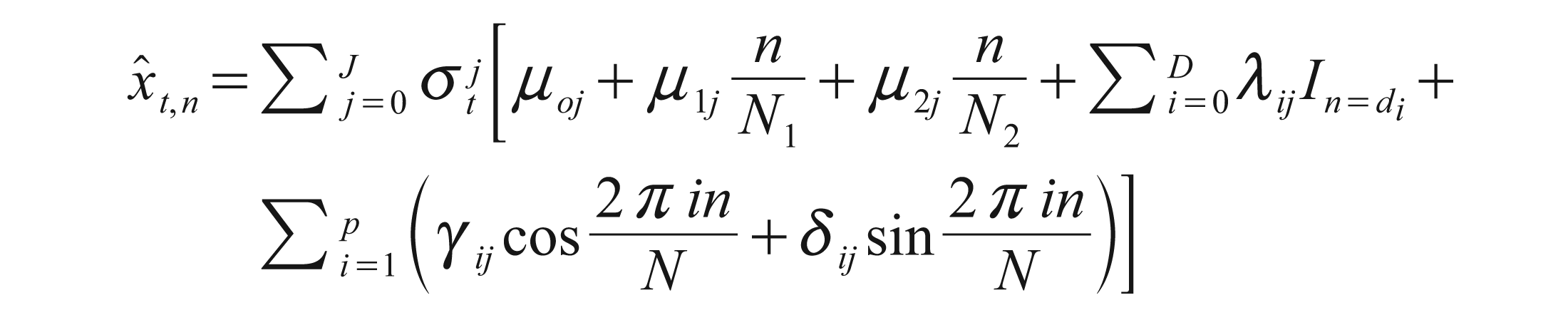
where P denotes the tuning parameter and refers to the order of expansion. P is chosen based on the information criteria such as Akike information criterion and Bayesian information criterion. N1 = (N+1)/2 and N2 = (N+1) (N+2)/2 are normalizing constants. Each of J+1 FFF are parameterized with the non-linear components in n (μ coefficients) and the number of sinusoids (γ and δ coefficients). J>0 allows the possible interaction between daily return volatility and periodic components. λ ij is the coefficient corresponding to dummies which may be introduced in the time interval during a day, corresponds to calendar events or news announcements. The value of J is determined on the basis of the best fit of the intraday periodic component, information criteria and the parsimony of the model.
Intraday periodic component is estimated as follows:

The filtered return series is obtained by normalizing the returns with the estimated periodic component as

Although the FFF method provides a parsimonious model, but it is not flexible in its functional form and assumes equality at the starting and closing of the periodic cycle (Taylor, 2004a). On the other hand, cubic spline allows for sharp peaks and troughs observed in a time series (Evans & Speight, 2010)
In the cubic spline approach, intraday periodicity patterns are obtained by fitting a three-degree polynomial between the predefined points called ‘knots’. Knots are positioned in such a way so as it can capture the complexities in intraday periodicities, for example, knots may be positioned at the opening and closing of dominant markets to capture the opening and closing effects of those markets. Following Evans and Speight (2010), operational regression equation to estimate the intraday periodicity component can be written as
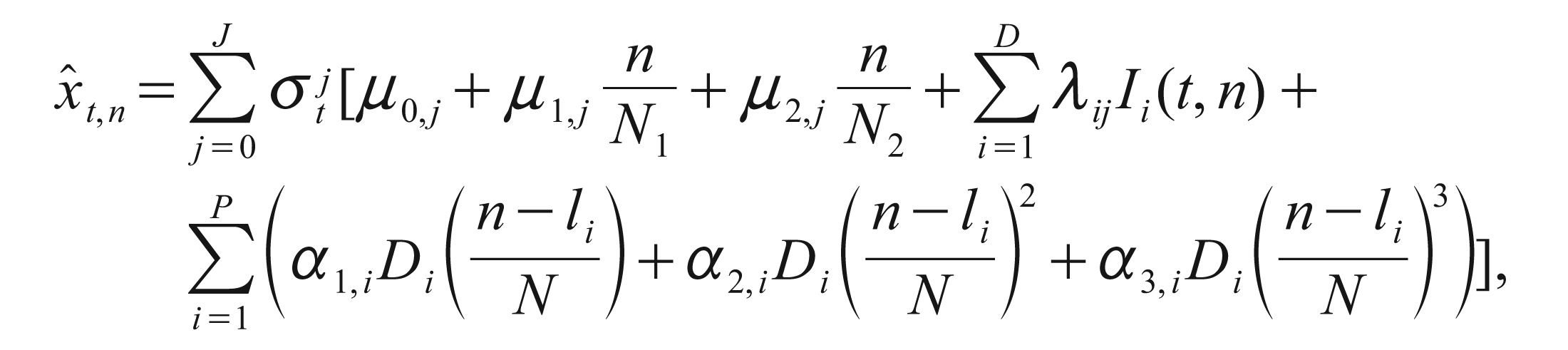
where N1 = (N+1)/2 and N2 = (N+1) (N+2)/2 are normalizing constants. li denotes the interval during the day in which ith knot (i=1,2,…,P) is placed. Di’s are dummy variables assigned the value one if li > n, otherwise zero. N is the number of intervals during the trading day. α1,i, α2,i, α3,i are the coefficients to be estimated. Ii(t,n) is the dummy variable taking the value of 1 for any calendar effect that occurs on day t and macroeconomic announcements that occurs at the nth interval on the tth day.
We employ five knots during the trading hours in order to capture the deterministic periodicity component. The first knot is positioned corresponding to the opening of the Indian commodity market at 10:00
Nelson (1991) proposed an exponential-GARCH (EGARCH) model where conditional variance is a function of past residuals and conditional variance. Nelson assumed that the errors follow a generalized error distribution (GED). He also pointed out that the use of GED improves the estimates of models in the presence of high kurtosis and fat-tails, which are the stylized facts of the return series. The conditional variance equation of the EGARCH model can be expressed as

The EGARCH model has several advantages over the GARCH models. First, there is no need to impose restrictions to ensure non-negativity in the parameters since it always provides a positive conditional variance (Brooks, 2008). Second, the asymmetric effect or leverage effect, that is, higher volatility levels observed following the negative shocks as compared to positive shocks, can be tested through this model. Haniff and Pok (2010) pointed out that EGARCH produced superior results compared to other GARCH and threshold GARCH (TGARCH) models. In this study, we have implemented two approaches—a sequential estimation approach and PGARCH models augmented with the FFF and cubic spline for volatility forecasting.
Andersen and Bollerslev (1997) proposed a ‘sequential estimation approach’ or ‘two-step method’ by making use of the FFF to estimate the conditional volatility. In the first step, which is the filtration of raw returns, the periodicity component is estimated and removed from the raw returns. In the second step, filtered returns are modelled with conventional volatility models, like GARCH and readjusted for periodicity. We make use of FFF and cubic spline to estimate the intraday periodicities in return volatility and to get filtered returns.
Periodic Models
Bollerslev and Ghysels (1996) proposed periodic-GARCH (PGARCH) allow the time dependency and periodicity in the conditional variance terms of GARCH model. Variance equation for the PGARCH model can be expressed as

where s(t) denotes the stage of the periodic cycle. Within periodic cycles, a periodic model allows the coefficients in the variance equation to take a different value in each period where the change in volatility is expected. One way to do this is with the inclusion of a set of dummy variables. Taylor (2004a) mentioned that, ‘these models are computationally expensive and are required to estimate a large number of parameters if there are many time periods within the periodic cycle’.
Haniff and Pok (2010) used a periodic version for the EGARCH models and found that EGARCH models provide a better fit than the GARCH and TGARCH models. The FFF and cubic spline versions of the PGARCH models are discussed in the following two sections:
The intraday periodic component can be introduced in the variance equation of Bollerslev and Ghysels’ (1996) periodic models without complicating the volatility estimation process (Haniff & Pok, 2010; Taylor, 2004a). The conditional variance equation in this framework can be expressed as


jϵ (1, 2, … J) denotes the intraday periodic cycle which may be chosen on the basis of the information criteria. N is the number of intervals during the trading day. S (t) denotes the tth interval. 5
The conditional volatility equation of cubic spline version of the periodic model in the EGARCH framework can be expressed as
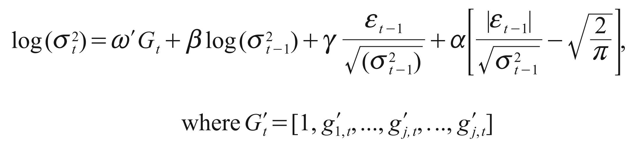
and

where lm denotes the interval of the day in which knot m (m=1,2, …, M) is placed, the knots are chosen by a priori-based criteria on the underlying intraday pattern in volatility or according to the expected change in intraday return volatility. 6
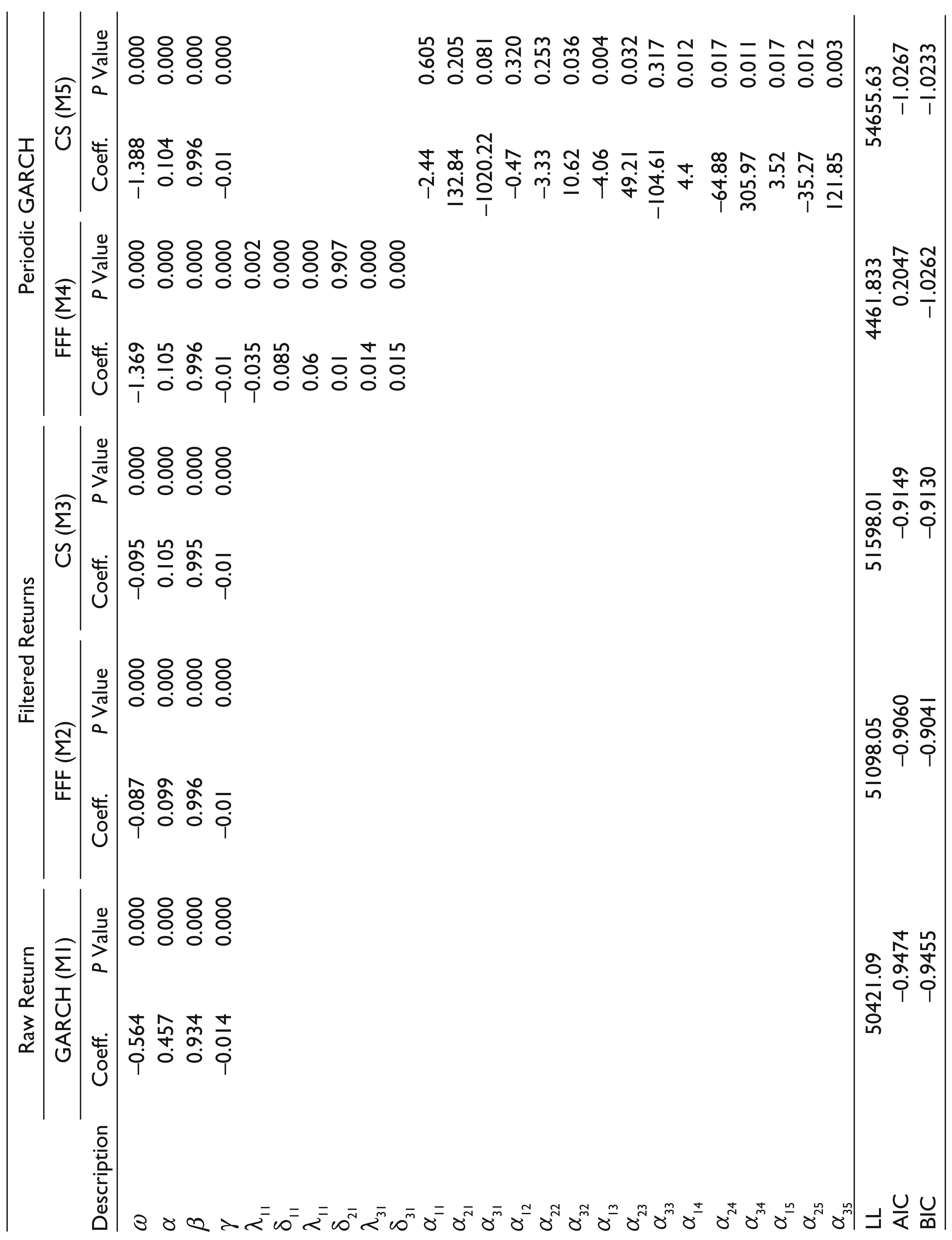
We determine the best model among the all five fitted models by comparing the in-sample model-fit and out-of-sample forecasting performance. 7 For the in-sample fit, we use three criteria: log likelihood (LL), Akaike information criterion (AIC) and Bayesian information criterion (BIC). The model which produces the maximum LL and minimum AIC and BIC among the competing models is considered best.
Accurate forecasting of the return volatility is important given its application in risk management and asset pricing. The model that provides forecasts of return volatility nearest to the realized volatility is considered the best. We compared all five models with the realized volatility. We considered absolute returns as a measure of realized volatility since it is less affected with the outliers. These outliers occur occasionally and they cannot be assumed repetitive over time (Martens, Chang, & Taylor, 2002).
We use several performance measures to ensure the robustness of the results. First, we compare the correlation between realized volatility and forecasted volatility. Second, we compare the mean forecast with the average forecast in the forecasted period. Third, we compare the mean absolute error (MAE) for all the models. The model that produces the minimum MAE is considered the best forecasting model. The MAE for N*T forecasts can be expressed as

where
Fourth, we estimate the root mean squared forecast error (RMSE), the N*T forecasts RMSE is given as

Finally, we compare the model-based forecasts by using Diebold and Mariano’s (1995) asymptotic test. The Diebold and Mariano test provides a measure of predictive accuracy for two competing predictions for a given loss function, by comparing them with the actual time series (we use the MAE as the loss function). This test verifies the null hypothesis that forecasts if two competing models are equally accurate. The advantage of the Diebold and Mariano test is that it provides robust results in case of non-normal and serially correlated forecasts errors (Taylor, 2004a).
Results and Discussion
Estimation of Intraday Periodicities
Economic theories do not provide any theoretical prediction about the intraday periodicities. While modelling intraday periodicities using FFF, the choice of the number of sinusoids is important. We choose appropriate models based on information criteria such as the AICs and BICs. We compare the information criteria for intraday periodicities estimated by FFF and explained in a regression equation (3) in conjunction with equation (2) for different values of P from a grid (1 to 10) and for J=0. 8 For models with J=1, the model cannot be applied directly for forecasting intraday volatility since the future daily return also needs to be estimated. We ignore the interaction between daily return volatility and intraday periodicity for the parsimony of the model. 9
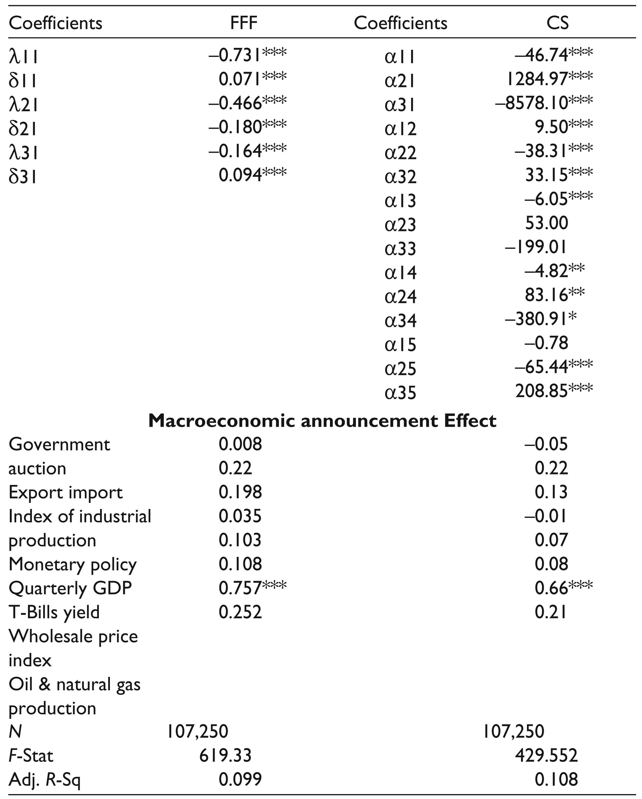
Figure 4 shows the intraday patterns in absolute returns estimated by using the FFF (left panel) and cubic spline (right panel) approach. It is apparent that both FFF and cubic spline provides a close fit over average intraday periodicity patterns. Table 2 provides the estimate of FFF and cubic spline coefficients, the calendar effect and macroeconomic announcements. 10 A high F-statistic indicates the presence of recurring and consistent patterns in volatility. The adjusted R-squares obtained by the cubic spline (0.107) method is higher than the FFF (0.099), which indicates that cubic spline provides a better fit for the intraday periodicities.
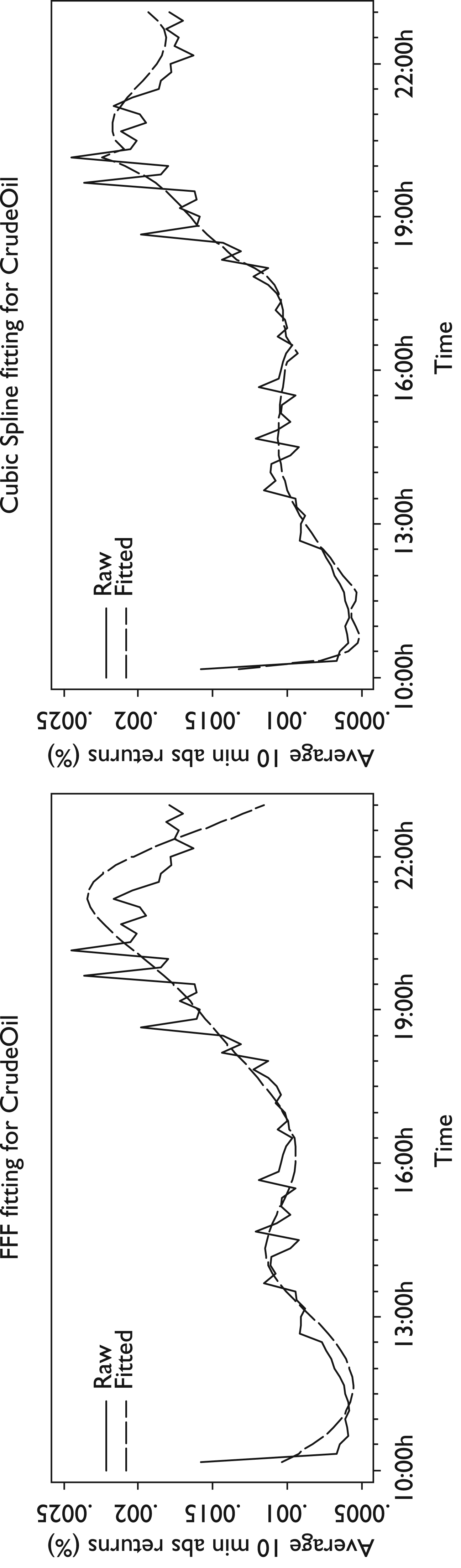
Figure 5 shows the 5-day correlogram for raw absolute returns |Rt,n| (left panels) and filtered absolute returns
Estimated Coefficients by Using FFF and Cubic Spline
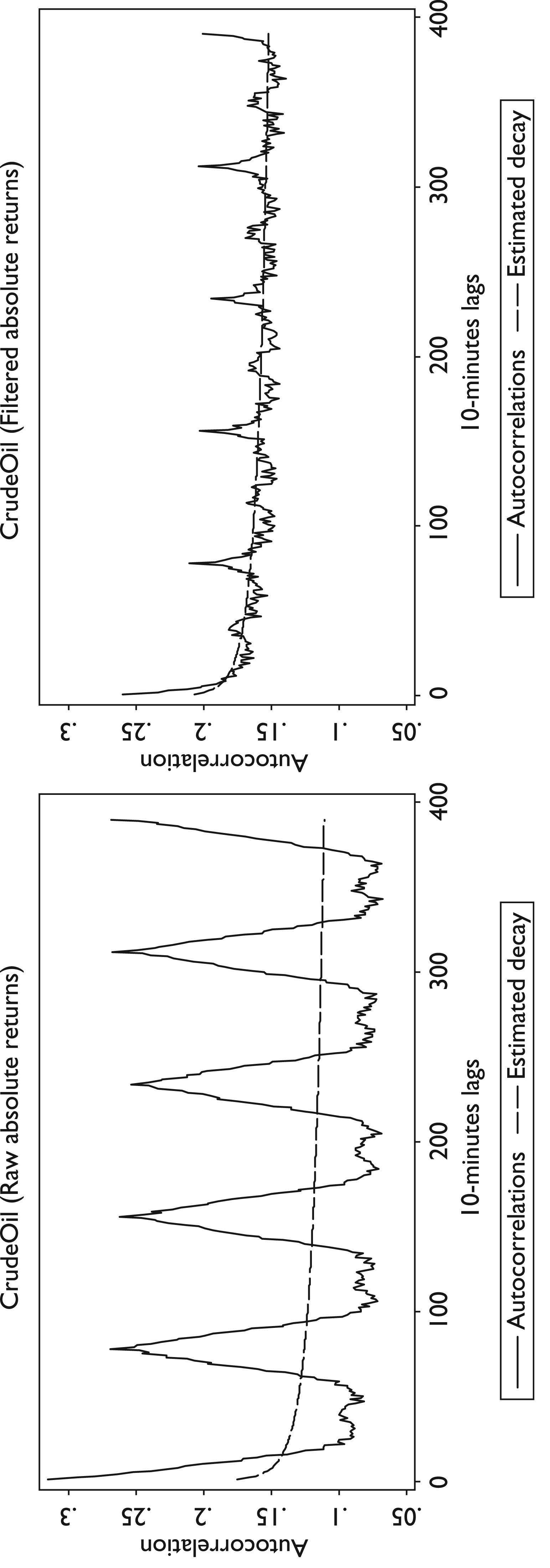

The correlogram for the raw returns (left panels) shows the presence of strong cyclical patterns. These cyclical patterns almost disappeared in the correlogram for filtered returns (right panels). The correlogram for filtered returns (right panels) shows that the 5-day correlogram is very close to the theoretical hyperbolic decaying patterns indicating that high-frequency returns exhibit high volatility persistence.
The filtration of high-frequency absolute returns determined by using FFF and cubic spline reveal interesting characteristics. After the adjustments for intraday periodicities, a long memory feature in the intraday return process emerges as an inherent feature of the return process. This reflects the importance of intraday periodicities in revealing the true characteristics of the returns. Furthermore, it is also important to test if the removal of intraday periodicities in return volatility results in a consistent parameter estimation of the conditional volatility models.
The presence of strictly positive autocorrelations and hyperbolic declining patterns in the correlation allow for estimating the degree of volatility persistence or the parameter of fractional integration (denoted by ‘d’). The relationship between autocorrelations ρj, of a long-memory process for large lags j, can be expressed as ρj ≈ cj2d–1 where c denotes the factor of proportionality (Bollerslev et al., 2000). The operational regression equation to estimate the fractional integration parameter is

Estimates of the fractional integration parameter are between (–0.5, 0.5) which shows that returns are neither stationary I (0) nor of order I (1). The value of the parameter of fractional integration d’s comes out to be 0.475.
Out-of-Sample Forecast
The estimated coefficients associated with non-periodic (M1), sequential models (M2 and M3) and periodic models (M4 and M5) are used to generate 10-minute return volatility forecasts for all the intervals during a trading day. Table 3 reports the estimated coefficients of FFF and cubic spline for the in-sample period. Intraday and interday periodicities in volatility estimated for the in-sample period are assumed consistent for the out-of-sample period.
In-sample Fit
In-sample Fit
The EGARCH (1,1) parameters for each model (M1 to M5) are re-estimated after each trading day (i.e., after 78, 10-minute intervals) using a rolling window of one year which constitutes around 250 days, starting from July 1, 2009 to June 30, 2010. The volatility forecast for 100 days starting from July 1, 2010 has been forecasted. This generates 7,800 forecasts.
The relative performances of all the models are compared by using four measures, which include correlation between forecasted volatility and realized volatility, mean forecast, MAE and root mean squared error (RMSE). We also make use of the asymptotic test proposed by Diebold and Mariano (1995). Table 4 reports the outcome of the mean forecast, correlation with the realized volatility, MAE and RMSE.
Out-of-sample Forecasting Performance
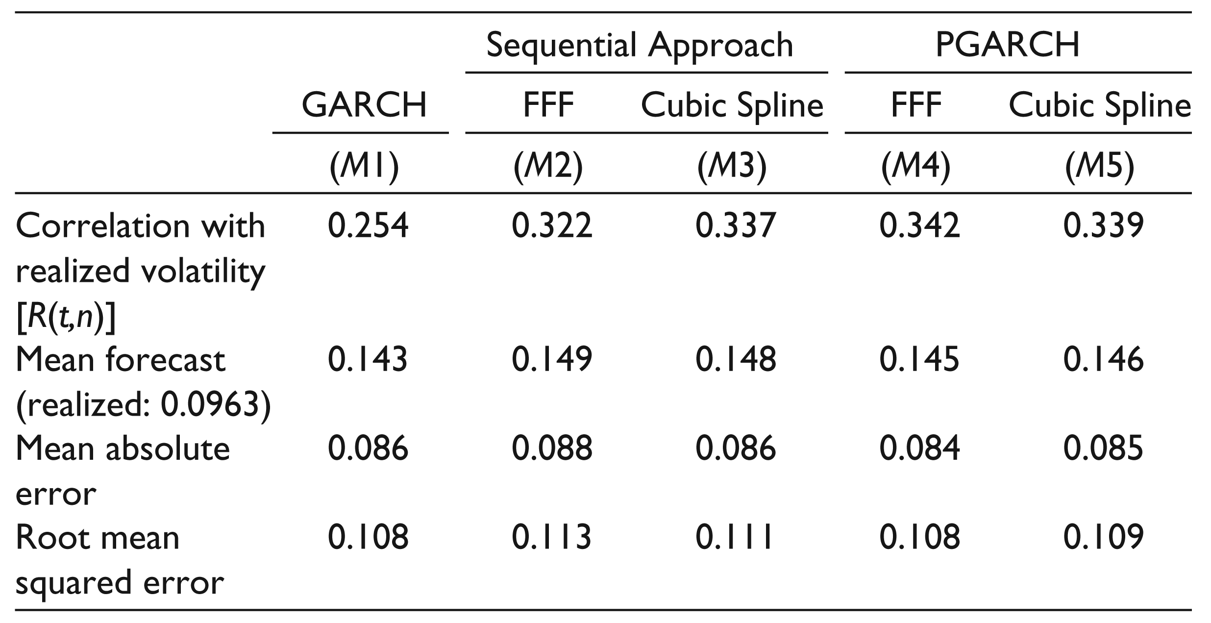
The non-periodic EGARCH model as evidenced by MAE, RMSE provide the worst out-of-sample forecasts compared to the sequential and periodic models. Forecasts obtained by the sequential estimation approach, particularly the cubic spline version (M3), is far better than the non-periodic model (M1), since the correlation between the estimated volatility and realized volatility increases from 0.25 to 0.33. The periodic models (M4 and M5) even perform marginally better than the sequential models (M2 and M3). The FFF version of the periodic model (M4) produces a minimum MAE and RMSE. However, the MAE and RMSE are very close across the models; therefore, to conclude which model is better, we need to test the statistical significance of difference between the MAE produced by the different models. Finally, we employ the Diebold and Mariano asymptotic test and to compare the forecasting performance of all the five competing models, where MAE is considered as the loss function. The main advantage of the Diebold and Mariano test is that it is robust enough to account for serially correlated and non-normally distributed errors (Taylor, 2004a). The results obtained from the Diebold–Mariano test are given in Table 5 with the corresponding level of significance (p values). It is apparent that the FFF and cubic spline versions of the PGARCH model outperform the non-periodic (M1) models and sequential models (M2 & M3).
Diebold and Mariano Test to Measure Relative Forecasting Performance

In this study, we have provided an extensive analysis of intraday periodicities in volatility by using intraday data for crude oil futures contracts traded at MCX, a leading commodity exchange in India. We implemented a FFF and cubic spline approach to estimate the intraday periodicity. Our findings suggest the presence of a deterministic and consistent intraday periodicity has strong impact on the characteristics of high-frequency returns. Filtration of the raw returns reveals the long memory property of volatility.
Further, we examined whether an adjustment for interday and intraday periodicities in commodity futures improve out-of-sample forecasts. We compared the forecasting performance of two versions of Andersen and Bollerslev’s (1997) sequential estimation models and two versions of Bollerslev and Ghysels’ (1996) periodic models with the EGARCH model. In order to arrive at the best model, we compared the forecasting performance of all five competing models by using four performance measures—correlation between forecasted volatility with realized volatility, mean forecast, MAE, RMSE, and the Diebold–Mariano test. Our findings show that the PGARCH model is marginally better than sequential estimation models. Our results are robust after controlling for time to maturity, seasonality, and macroeconomic announcements. Our findings have implications for portfolio management.
Footnotes
Acknowledgements
The authors are grateful to MCX, in particular V. Shunmugam for the data and Arindam Ghosh for explaining the data and the workings of the futures market to us. The contents of the paper including the conclusions do not reflect the opinions of MCX or any of its officers, employees, or associates. The authors are solely responsible for any error.