Statistical Arbitrage Strategies under Different Market Conditions: The Case of the Greek Banking Sector

Abstract

In this article, we examine the behaviour of cointegration-based pairs trading (PT) strategies, under different market conditions. Reported results indicate that changes in market conditions affect the stability of long-run relations between pairs of stocks, therefore suggesting that arbitrageurs should perform rebalancing between the examined stocks when a change in market trend is evident. The applicability of our results may be of importance to market participants; although cointegration applications have received considerable attention from hedge funds adopting statistical arbitrage (SA) strategies, little evidence has been reported for the validity of these trading strategies under changing market conditions.

JEL Classification: C32, G11

Keywords

Cointegration pairs trading strategies market conditions

1. Introduction and Literature Review

Compared with previous research, the present study aims to extend existing literature by considering whether changes in market performance alternate the mean-reverting properties of long-run relations between equities and, as a result, affect implementation of pairs trading (PT) strategies. Since the cointegration approach is widely used by hedge funds adopting statistical arbitrage (SA) or PT strategies, we believe our results are of significant importance, suggesting that when a change in market performance is evident, then fund managers should keep in mind the necessity of rebalancing.

The examined data set contains a sharp downtrend phase followed by a moderate uptrend period. Employing cointegration analysis, reported results initially indicate that changes in market performance affect the stability of long-run relations, therefore suggesting that arbitrageurs should perform rebalancing among the examined shares when there is a change in the market trend. Furthermore, according to our statistical results, intense market conditions harm the mean-reverting properties of the long-run relations, which have been identified in our full sample analysis, while a moderate market performance points to cointegration between the examined stocks in each pair. In such a moderate market phase, the presence of a stationary spread suggests the potential of abnormal short-run returns realisation, through exploitation of deviations from its mean value.

The present study, in this respect, pertains to the examination of a market efficiency issue, considering pairwise long-run relations between bank shares trading in the Greek stock market,¹ under different market conditions, and the implications of these relations on the implementation of PT strategies. There is considerable literature in financial economics concerning the validity of various forms of the efficient market hypothesis (EMH); Cuthbertson (1996) provides a thorough review. The EMH implies that in liquid markets, where asset prices will be the result of unconstrained demand and supply equilibria, the current price should accurately reflect all the information that is available to the markets participants.

In an efficient market, the fair game² model holds for stock price changes:

E [P_{t} - (P_{t}^{*} | I_{t - 1})] = 0

where I_{t −1} is the information set available at time t −1, P_t is the actual price at time t , P_t^* is the expected price which is based on the information set I_{t −1} and P_t−P_t^* is the forecast error which is uncorrelated with variables in the information set I_{t −1}. Obviously, the same model holds for stock returns (r_t ) as returns are a transformation of price changes.³

Statistically, the model that is most commonly assumed for stock price movement is a log-normal process; that is, the logarithm of the stock price is assumed to exhibit a random walk. However, because the random walk is a martingale, the mean value of the predicted increment is zero. Therefore, knowing the past history of a random walk is not much help in predicting the forward-looking increments. The condition is very different for stationary processes. Armed with the knowledge that stationary processes are mean reverting, one can predict the increment to be greater than or equal to the difference between the current value and the mean. The aforementioned prediction is guaranteed to hold true at some point in the future realisations of the time series.

Given that stock price predictability may lead to abnormal returns, testing mean reversion has been the objective of many researchers since the 1960s. While initial studies (Fama, 1965; Samuelson, 1965; Working, 1960) could not reject the random walk hypothesis, later findings are mixed. Some studies suggest stock prices are either mean reverting (Balvers, Wu, & Gilliland, 2000; Chaudhuri & Wu, 2003a, 2003b; Fama & French 1988; Grieb & Reyes, 1999; Lo & MacKinlay, 1988; Poterba & Summers, 1988; Urrutia, 1995) or random walk processes (Choudhry, 1997; Huber, 1997; Kawakatsu & Morey, 1999; Liu, Song, & Romilly, 1997; P. K. Narayan & S. Narayan, 2007; Narayan & Smyth, 2004, 2007; Zhu, 1998). However, recent research evidence suggests the existence of stationary linear relations among log data of share prices. Based on this result, it is suggested the construction of SA strategies⁴ exploiting the mean-reverting properties of linear relations among financial data (Alexakis, 2010; Bondarenko, 2003; Canjels, Prakash-Canjels, & Taylor, 2004; Forbes, Kalb, & Kofman, 1999; Harasty & Roulet, 2000; Hogan, Jarrow, Teo, & Warachka, 2004; Jacobsen, 2008; Laopodis & Sawhney, 2002; Mavrakis, 2011; Tatom, 2002; Wang & Yau, 1994).

The SA techniques are widely used by hedge funds, Wall Street companies and even sophisticated independent investors trying to profit from temporary deviations of equity prices from their fundamental value. In academic literature, SA is opposed to arbitrage (deterministic). In deterministic arbitrage, a sure profit can be obtained from being long in some securities and short in others. In SA, there is a statistical mispricing of one or more assets based on the expected value of these assets. In other words, SA conjectures statistical mispricing or price relationships that are true in expectation, in the long run, when repeating a trading strategy.

One of the most popular SA trading strategies is PT. The PT is a simple trading strategy that aims to exploit temporal deviations from an equilibrium price relationship between two securities. This is given by a long position in one security and a short position in another security in such a way that the resulting portfolio is market neutral (which typically translates in having a beta equal to zero). This portfolio is often called a spread. The PT is a very simple technique and as Pole puts it: ‘ find two stocks whose prices have historically moved together, when the spread between the two widens, short the winner and buy the loser; if history repeats itself, prices will converge and the arbitrageur will profit’ (Pole, 2007). According to Gori (2009), in the framework of spread modelling, among the more recent techniques, we find that cointegration is probably the most popular approach⁵ in quantitative trading strategies adopted by hedge funds and a significant number of studies have been published on it. Bondarenko (2003) and Hogan et al. (2004) defined SA as an attempt to exploit the long-horizon trading opportunities revealed by cointegration relationships. Furthermore, according to Alexander and Dimitriu (2005), compared with other conventional methods, cointegration performs better as a way of applying SA strategies. Marshall, Nguyen and Visaltanachoti (2013), recognising the value of cointegration theory, use the error correction models (ECM) in order to recognise mispricing in ETFs allowing arbitrage opportunities. Caldeira and Moura (2013) also applied cointegration trading strategies in the Sao Paulo Stock Exchange with profitable results.

As suggested by Alexander (2001), the power of cointegration analysis is that optimal portfolios may be constructed on the basis of common long-run trends among asset prices, and they will not require extensive rebalancing. On the contrary, according to Lin, McCrae and Gulati (2006), arbitrage trading of the ‘convergence trade’ type is rarely riskless since market events or structural price changes may invalidate statistical pricing models, which may require parameter re-estimation. This is because price spreads, after position opening, may escalate rather than revert, or the equilibrium position may shift.

So far, in the relevant literature, there are rather conjectures (Alexander & Dimitriu, 2002; Lin et al., 2006) than evidences supporting the argument that changes in market performance alternate the mean-reverting properties of long-run relations between financial assets and, as a result, affect implementation of SA strategies on the variables under consideration. That is, there is small empirical evidence suggesting that arbitrageurs should perform rebalancing among the traded assets when a change in market performance is evident. Nevertheless, potential alternations under different market phases have been reported in several studies. In a relatively early study, Bhardwaj and Brooks (1993) find that significant firm-size-related differences in abnormal returns and systematic risks occur in ‘bull’ and ‘bear’ market months for NYSE and AMEX from 1926 to 1988. Meric, Ratner and Meric (2008) examine the portfolio diversification implications of the co-movements of sector indexes in the US, UK, German, French and Japanese stock markets in ‘bull’ and ‘bear’ markets. They find that, in a ‘bull’ market, investors can obtain more benefit with global diversification than with domestic diversification even if they invest in the same sector in different countries as opposed to investing in different sectors within the same country. In a ‘bear’ market, the sectors of different countries tend to be more closely correlated and country diversification opportunities are limited. Jansen and Tsai (2010) examined asymmetries in the impact of monetary policy surprises on stock returns between ‘bull’ and ‘bear’ markets in the period 1994–2005 in USA. According to their results, the impact of a surprise policy action in a ‘bear’ market for most industries is significantly greater than the impact of surprise monetary policy in a ‘bull’ market. Cheng, Lee and Lin (2013) examine the magnitude of the disposition effect between ‘bear’ and ‘bull’ markets and find that in the ‘bear’ market, there is a stronger disposition effect.

Thus, empirical research evidence drove us to examine pair SA strategies under different market conditions. The main objective of the present study is to contribute in the relevant literature, shedding more light on the effects of changes in market conditions on the formation of SA strategies which rely on the cointegration approach. Thus, we will examine whether changes in market performance alternate the mean-reverting properties of long-run relations between equities and, as a result, affect implementation of PT strategies on the stocks under consideration.⁶ The international evidence in this direction is very limited, although there are some studies; according to Miao (2014), a cointegration-based trading system performed well in and out of the sample testing, even in periods when negative returns were dominant in the market, leading to the conclusion that ‘the developed trading system may be more profitable when the stock market performs poorly’.

The remainder of this article includes a description of the examined data, in the second section, and research organisation along with the employed methodology, in the third section, followed by model specification and results on cointegration rank tests as well as tested hypotheses, in the fourth section. Finally, the fifth section provides a summary and conclusions.

2. Data Description

Data employed in this article include weekly closing prices of six banks’ equity shares quoted in the Greek stock market. In order to leave out any structural effects arising from the introduction of Euro as well as turbulent periods that followed the 2008 financial crisis, we choose to examine a 7-year period, from 5 January 2001 to 28 December 2007. The examined Greek stocks are as follows: National Bank, Alpha Bank, Bank of Cyprus, EFG Eurobank Ergasias, Piraeus Bank and Marfin Bank. Our choice of stock prices variables relies on our objective to examine all possible shares constituting the banks’ sector index in the Greek market as well as on the availability of data for the examined 7-year period. Apart from the banks’ sector index, the examined shares are also included in one popular market performance index, namely, the FTSE/ASE 20 for the Greek market.

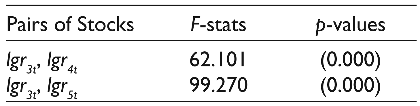
In order to examine pairwise cointegrating relations between the examined equity shares under different market conditions, we have split the sample into two subsamples. We can visually examine, in Figure 1, the performance of the FTSE/ASE 20 index for the examined 7-year period. Although structural change is obvious from visual inspection of data in Figure 1, in order to further justify our choice to split the sample, we apply a breakpoint test suggested by Chow (1960). The breakpoint test is applied on a linear regression of the relationship between log price data of those pairs of stocks that appear to be cointegrated in the first part of our econometric analysis where we have employed full sample data. According to the results of the Chow test in Table 1, with a zero p -value, we reject the null of no breaks at the starting point of the second subsample, in all cases. In addition, to the latter documentation of the two subsamples, in order to reveal market performance, we define positive (negative) weekly index returns as Up (Down) market returns. Furthermore, following Fabozzi and Francis (1977), we redefine Up (Down) market returns as Substantially Up (Substantially Down) market returns when the weekly return of an index is larger (lower) than the sum (difference) between average market return and half of one standard deviation measured over the full sample.

Figure 1.

Source: Datastream.

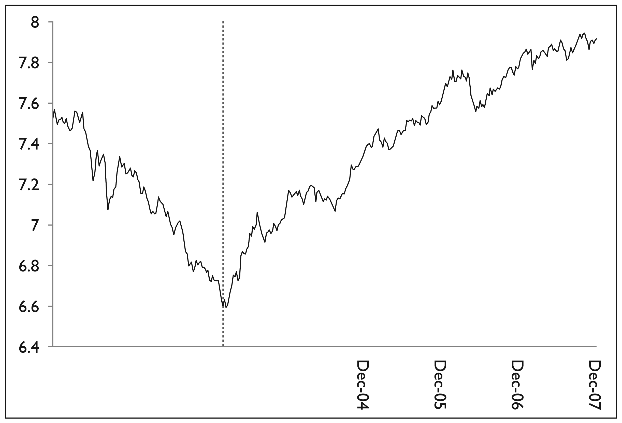
Examining market performance of the Greek FTSE/ASE 20 index, in the first subsample, there are 47 Up and 68 Down market returns, while 73.53 per cent of the Down returns are also Substantially Down market returns. In the second subsample, there are 149 Up and 101 Down market returns, while 53.69 per cent of the Up returns are also Substantially Up market returns.

While there is no commonly agreed-upon definition for a ‘bear’ market, broadly defined, a ‘bear’ market represents a substantial decline of at least 20 per cent in stock prices over a period of several months. This characteristic is met in market performance of the FTSE/ASE 20 index in the first sub-period. Furthermore, in the first sub-period, we find that the number of Down returns characterised as Substantially Down returns is sufficiently higher than 50 per cent. In this way, we identify the first subsample as an intense period.

According to market analysts, a ‘bull’ market is a prolonged period in which share prices rise faster than their historical average. Considering market performance of the Greek FTSE/ASE 20 index, in the second sub-period, we find that the number of Up returns characterised as Substantially Up returns is 53.69 per cent. That is, the number of Up returns characterised as Substantially Up returns is slightly higher than 50 per cent. In this way, we identify the second subsample as a moderate period.

Table 1.

Chow’s Breakpoint Test

Pairs of Stocks	F-stats	p-values
lgr_3t, lgr_4t	62.101	(0.000)
lgr_3t, lgr_5t	99.270	(0.000)

Source: Datastream.

Note: Chow’s test for a breakpoint on 21 March 2003.

Overall, the sample under consideration contains a period of intense ‘bear’ market followed by a moderate ‘bull’ market. The intense period falls within the subsample from 5 January 2001 to 14 March 2003, and the data set includes 115 observations. The moderate period falls within the subsample from 21 March 2003 to 28 December 2007 and the data set includes 250 observations.

3. Methodology and Research Organisation

Our research schedule is comprised of three parts. First, employing full sample data, we investigate whether there are bivariate cointegrating relations among all the possible pairs of the examined shares. In the second part of our analysis, splitting the sample into two sub-periods, we examine whether market performance affects the statistical evidence of possible cointegrating relations, indicated by the results of the first empirical part. Finally, as indicated by the results of the second part, in the third empirical part, we shed more light on the second subsample, characterised as a moderate period, in order to reveal differences between cointegrating relations from full sample and second subsample data.

We apply the Johansen (1988, 1996) and Johansen and Juselius (1990) methodology of the cointegrated VAR model. As noted by Gonzalo (1994) and Kremers, Ericsson and Dolado (1992), the Johansen and Juselius approach performs better or at least as well as, the Dickey–Fuller cointegration test of Engle and Granger (1987). In addition, the selected procedure is invariant to different normalisations (Hamilton, 1994) and thus the test outcome does not depend on the chosen normalisation. Our results were obtained using CATS in RATS version 2 (Dennis, Hansen, Johansen, & Juselius, 2005). We choose to restrict the constant term, μ₀ , to lie in the cointegrating space and in addition, when proper, we include dummy variables, D_t , as unrestricted to the cointegrating space.

The error correction form of the examined unrestricted VAR model is described here:

\begin{matrix} Δ x_{t} = Π x_{t - 1} + \sum_{i = 1}^{k - 1} Γ_{i} Δ x_{t - i} + μ_{0} + φ D_{t} + ε_{t}, ε_{t} ~ N_{P} (0, Σ), \\ t = 1, ​ \dots, ​ T \end{matrix}

(1)

where x_t is a vector of two variables:

[l i_{t}, l j_{t}] ~ I (1),

(2)

li_t : weakly closing prices (in logs) of bank i ,

lj_t : weakly closing prices (in logs) of bank j ,

and D_t is a vector of deterministic variables such as intervention dummies.

Notation of the examined banks’ shares is as follows: lgr_1t for National Bank, lgr_2t for Alpha Bank, lgr_3t for Cyprus Bank, lgr_4t for EFG Eurobank Ergasias, lgr_5t for Piraeus Bank and lgr_6t for Marfin Bank.

Our choice to employ a model with a constant term and exclude the presence of a trend, in the examined log-run relations, is implied by the nature of PT as a SA strategy. That is, implementing a PT strategy, an arbitrageur forms a long/short portfolio of two assets, where the weights in each asset depend on the coefficients of the implied long-run relation between them. However, his initial decision to set up as well as the follow-up of such a portfolio relies on the statistical properties of the spread between the prices of these assets. Therefore, in order to set up such a strategy, the trader should initially verify the existence of a long-run relation as the one described in Equation (3).

l i_{t} = β \cdot l j_{t} + S p r e a d + s t a t . e r r o r

(3)

In other words, what an arbitrageur looks for is a stationary spread (li_t–β^–lj_t ). As stated by Pole (2007), relying on the stationarity of the spread between two assets, when detecting a divergence from its mean value then, the arbitrageur shorts the winner and buys the loser: if history repeats itself, prices will converge and the arbitrageur will profit. Alternatively, let as assume that, instead of employing the model described in Equation (1), we choose to include a trend in the cointegrating relation. Although we could have found a stationary long-run relation, however in that case the arbitrageur could not set up a strategy based on the stationarity of the spread (li_t–β^–lj_t ).

Implementing PT strategies and assuming that we have already choose the pairs of stocks then, we should identify the weights of the two assets, the so-called pair’s ratio. According to Gori (2009), this ratio should meet two requirements. First, it should make the strategy zero cost, and second, it needs to make the strategy market neutral (which typically translates in having a beta equal to zero). Consequently, in an estimate of a long-run relation as the one described in Equation (3), the presence of a slope coefficient significantly different from unity is justified and can be interpreted by the pair ratio.

Performing model specification, we choose the optimal number of lags using Schwarz, Hannan–Quinn and Akaike information criteria along with a likelihood ratio (LR) test. Following Juselius and MacDonald (2003), in order to secure valid statistical inference, we need to control for the largest of observations by dummy variables or omit the most volatile periods from our sample. Since the volatile periods could potentially be highly revelatory, we followed the Juselius and MacDonald approach. The dummy variables used in our models are permanent impulse dummies Dyyyy.mm.dd_t (equal to one at yyyy:mm:dd , and equal to zero otherwise).

Performing cointegration tests, our main objective is to investigate whether there is a long-run relation, with a non-zero intercept, between the examined banks’ shares in each pair. Applying Johansen (1988, 1996) and Johansen and Juselius (1990) methodology of the cointegrated VAR model, we examine the existence of a long-run relation with a non-zero intercept based upon the estimated eigenvalues, ${\hat{λ}}_{l}$ , and the trace test, τ_p–r .

In addition, we perform hypothesis testing regarding multivariate stationarity, univariate normality and variable exclusion. In the presence of I(1) series, Johansen and Juselius (1990) developed a multivariate stationarity test which has become the standard tool for determining the order of integration of the series within a multivariate context. The multivariate stationarity test is a LR test distributed as chi-square with (p–r ) degrees of freedom, [χ ²(1)_95% = 3.841]. Testing univariate normality, we apply the Doornik and Hansen (2008) test, distributed as χ ²(2), [χ ²(2)_95% = 5.991]. In order to test variable exclusion, we apply a LR test distributed as chi-square with r degrees of freedom.

Furthermore, focusing on the cointegrated pairs of banks’ shares, we perform long-run identification of the existent cointegrating relations through testing the validity of overidentifying restrictions. First, we test the null hypothesis of long-run weak exogeneity for each stock constituting the examined pair. According to Juselius (2006), the hypothesis that a variable has influenced the long-run stochastic path of the other variables of the system, while at the same time has not been influenced by them, is called the hypothesis of ‘no levels feedback’ or long-run weak exogeneity. The long-run weak exogeneity test is a LR test distributed as chi-square with r degrees of freedom. Second, testing whether cumulating shocks driving the system have exactly the same influence on both variables (li_t and lj_t ), we examine whether the hypothesis of long-run homogeneity holds. That is, we examine whether the cointegrating vector is (1, −1). Third, in cases where results, of long-run weak exogeneity test, point to the identification of the common stochastic trend, we apply a joint test of long-run weak exogeneity and long-run homogeneity hypotheses. Finally, in order to further justify our suggestions, we apply the augmented Dickey–Fuller (ADF) technique (Dickey & Fuller, 1981) to test the null hypothesis that the spread has a unit root.

4. Model Specification and Results on Cointegration Rank and Tested Hypotheses

As mentioned, performing model specification, we choose the optimal number of lags using Schwarz, Hannan–Quinn and Akaike information criteria along with a LR test while, in order to secure valid statistical inference, we choose to control for the largest of observations with the use of dummy variables.

In the first part of our analysis, examining full sample data, for 15 pairs of banks’ shares, we have employed a model with either one or two lags, described in Equation (4).

Δ x_{t} = α (β^{'}, ρ^{'}) (\begin{matrix} x_{t - 1} \\ 1 \end{matrix}) + \sum_{i = 1}^{k - 1} Γ_{i} Δ x_{t - i} + μ_{0} + φ D_{t} + ε_{t}

(4)

where k equals the number of lags minus one.

Being sufficiently confident about the specification of our model, we shall try to determine the rank. Reported results, in Tables 2a–2e, suggest in two cases rejection of the null hypothesis of r = 0 while a cointegration rank equal to one is accepted, with 95 per cent significance. Overall, for the pairs of (a) lgr_3t–lgr_4t , and (b) lgr_3t–lgr_5t , we have evidence that our system contains one cointegrating relation and, as a result, one common trend.

Considering results reported in Tables 2a–2e, further analysing the two cointegrated pairs [(a) lgr_3t–lgr_4t , and (b) lgr_3t–lgr_5t ], with rank = 1, we cannot accept the exclusion of any of the variables of the system. Overall, in both cases, we have a system where the employed variables are non-stationary and significant; therefore, they cannot be excluded. Univariate normality test outcomes suggest that residual properties are within acceptable levels. The rest of our analysis, in this part, is focused on the two cointegrated pairs. That is, as described further, performing detailed long-run identification we shall test the validity of overidentifying restrictions on the implied cointegrated vectors.

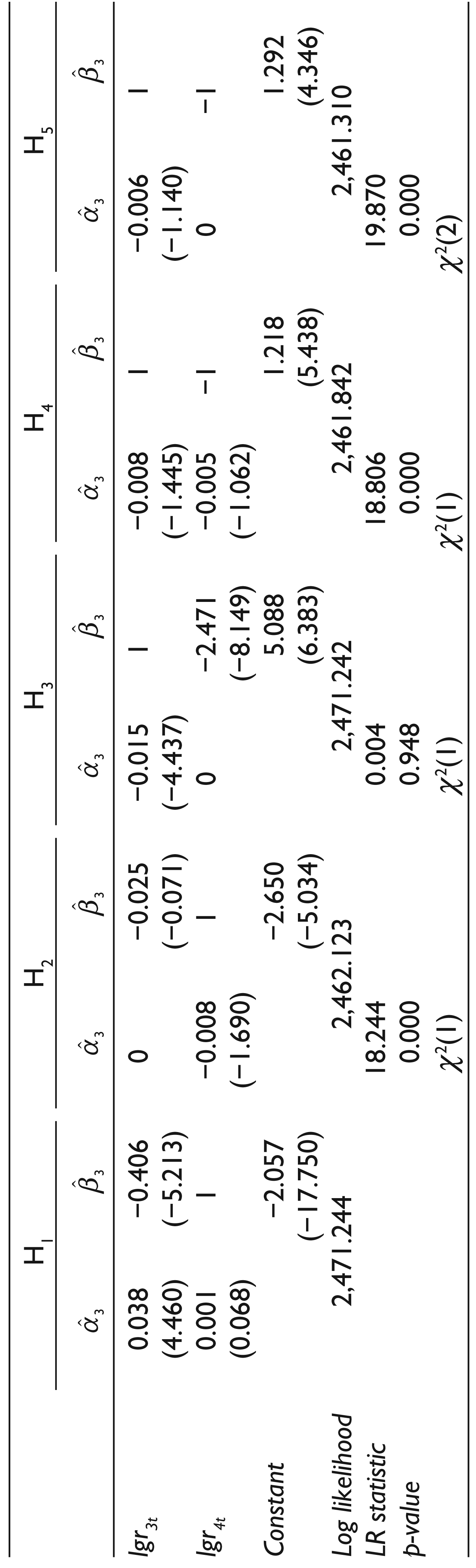
Examining the dynamics of each system, we perform hypothesis testing. We begin our analysis, in Tables 3a and 3b, with the unrestricted model Η₁. We choose to normalise the β vector to lgr_4t in the first case (Table 3a), and to lgr_5t in the second case (Table 3b). Although normalisation of these cointegrated vectors leads to two identified cointegrating relations, we choose to impose overidentifying restrictions.

Table 2a.

Bivariate Trace Tests for Cointegration Rank and Hypothesis Testing (Full Sample)

# lags	r	p–r	i	${\hat{λ}}_{l}$	τ_p–r	C_95%(p–r)	lgr_1t	lgr_2t
1	0	2	1	0.042	16.144^b	20.164	14.468^i,a	13.013^i,a
	1	1	2	0.001	0.368^b	9.142	2.455^ii,b	0.273^ii,b
							13.013^iii,a	14.468^iii,a
# lags	r	p–r	i	${\hat{λ}}_{l}$	τ_p–r	C_95%(p–r)	lgr_1t	lgr_3t
1	0	2	1	0.049	18.783^b	20.164	9.907^i,a	17.319^i,a
	1	1	2	0.002	0.603^b	9.142	1.638^ii,b	3.088^ii,b
							17.319^iii,a	9.907^iii,a
# lags	r	p–r	i	${\hat{λ}}_{l}$	τ_p–r	C_95%(p–r)	lgr_1t	lgr_4t
1	0	2	1	0.026	10.963^b	20.164	8.123^i,a	7.692^i,a
	1	1	2	0.003	1.263^b	9.142	0.953^ii,b	0.342^ii,b
							7.692^iii,a	8.123^iii,a
# lags	r	p–r	i	${\hat{λ}}_{l}$	τ_p–r	C_95%(p–r)	lgr_1t	lgr_5t
2	0	2	1	0.014	7.060^b	20.164	2.443^i,b	2.083^i,b
	1	1	2	0.005	1.975^b	9.142	1.610^ii,b	0.391^ii,b
							2.083^iii,b	2.443^iii,b
# lags	r	p–r	i	${\hat{λ}}_{l}$	τ_p–r	C_95%(p–r)	lgr_1t	lgr_6t
2	0	2	1	0.026	12.496^b	20.164	2.825^i,b	2.469^i,b
	1	1	2	0.008	2.902^b	9.142	1.791^ii,b	1.355^ii,b
							2.469^iii,b	2.825^iii,b

Source: Datastream.

Notes: 1. ^a Rejection of the null with 95 per cent significance.

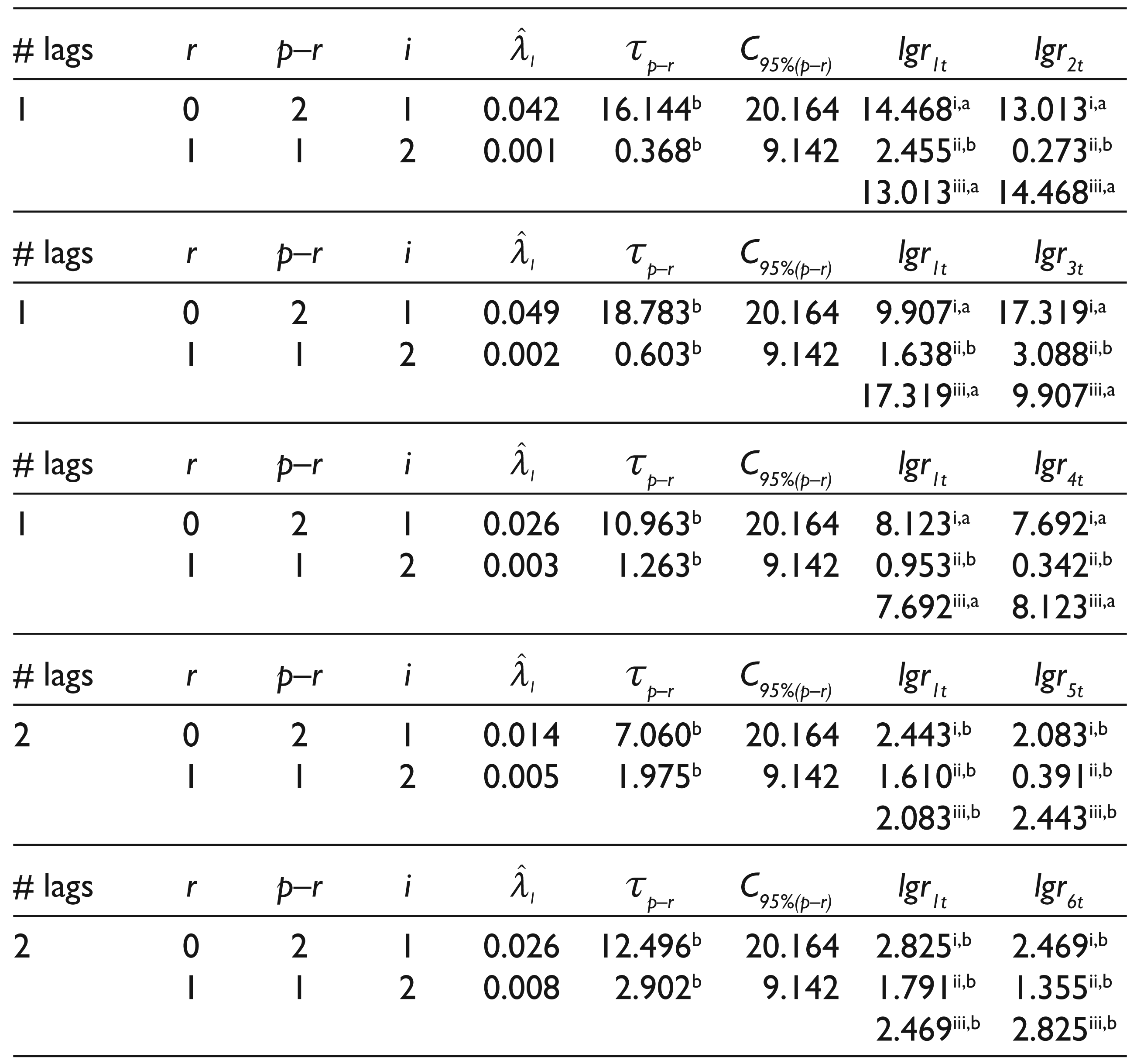
2. ^b Acceptance of the null with 95 per cent significance.

3. ⁱ Multivariate Stationarity test is a LR test, distributed as χ ²(1).

4. ⁱⁱ Doornik and Hansen (2008) univariate normality test, distributed as χ ²(2).

5. ⁱⁱⁱ Variable Exclusion is a LR test, distributed as χ ²(1).

Table 2b.

Bivariate Trace Tests for Cointegration Rank and Hypothesis Testing (Full Sample)

# lags	r	p–r	i	${\hat{λ}}_{l}$	τ_p–r	C_95%(p–r)	lgr_2t	lgr_3t
2	0	2	1	0.052	19.285^b	20.164	4.996^i,a	15.786^i,a
	1	1	2	0.000	0.051^b	9.142	1.043^ii,b	2.334^ii,b
							15.786^iii,a	4.996^iii,b
# lags	r	p–r	i	${\hat{λ}}_{l}$	τ_p–r	C_95%(p–r)	lgr_2t	lgr_4t
1	0	2	1	0.022	8.843^b	20.164	7.491^i,a	7.457^i,a
	1	1	2	0.002	0.652^b	9.142	0.644^ii,b	1.532^ii,b
							7.457^iii,a	7.491^iii,a
# lags	r	p–r	i	${\hat{λ}}_{l}$	τ_p–r	C_95%(p–r)	lgr_2t	lgr_5t
1	0	2	1	0.023	9.697^b	20.164	4.284^i,a	5.600^i,a
	1	1	2	0.003	1.185^b	9.142	0.470^ii,b	3.588^ii,b
							5.600^iii,a	4.284^iii,a
# lags	r	p–r	i	${\hat{λ}}_{l}$	τ_p–r	C_95%(p–r)	lgr_2t	lgr_6t
2	0	2	1	0.021	10.772^b	20.164	2.149^i,b	1.729^i,b
	1	1	2	0.008	2.893^b	9.142	0.658^ii,b	2.274^ii,b
							1.729^iii,b	2.149^iii,b

Source: Datastream.

Notes: ^a Rejection of the null with 95 per cent significance.

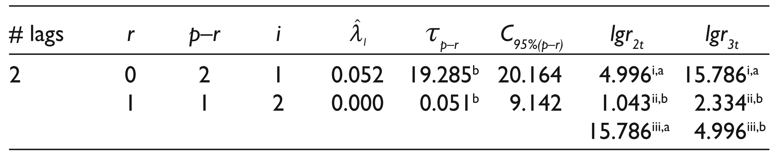
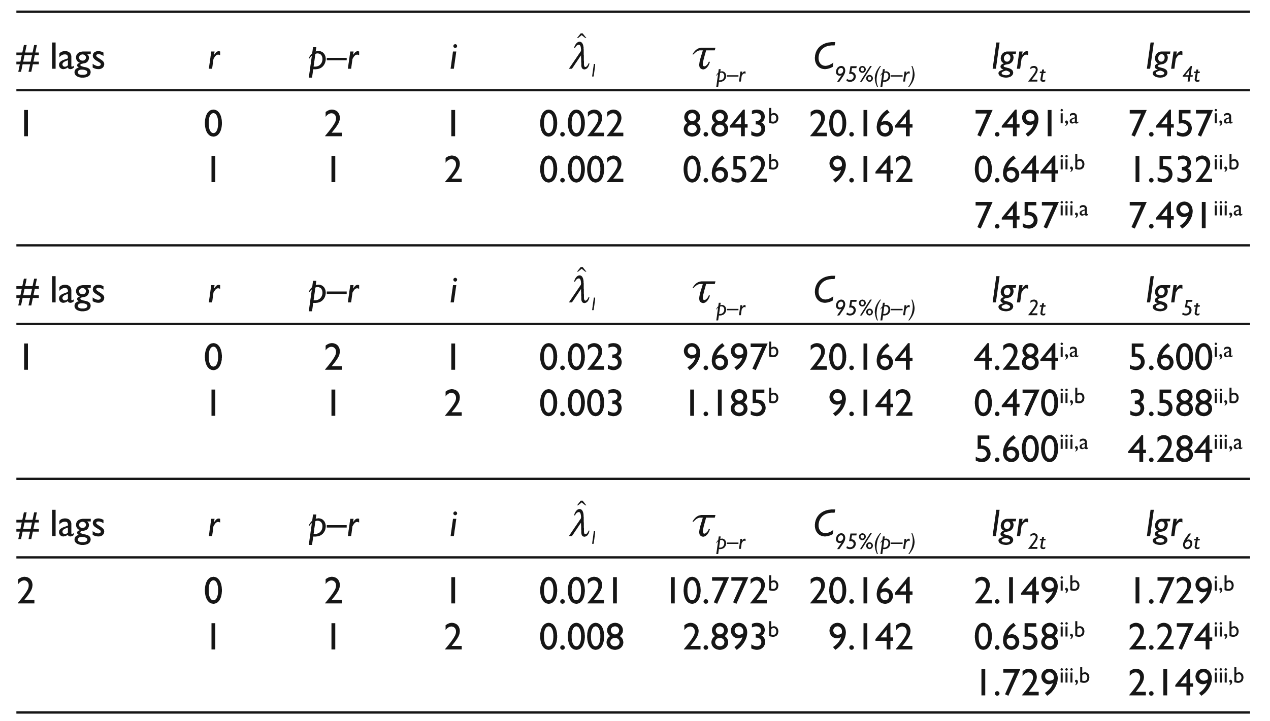
^b Acceptance of the null with 95 per cent significance.

ⁱ Multivariate stationarity test is a LR test, distributed as χ ²(1).

ⁱⁱ Doornik and Hansen (2008) univariate normality test, distributed as χ ²(2).

ⁱⁱⁱ Variable exclusion is a LR test, distributed as χ ²(1).

Table 2c.

Bivariate Trace Tests for Cointegration Rank and Hypothesis Testing (Full Sample)

# lags	r	p–r	i	${\hat{λ}}_{l}$	τ_p–r	C_95%(p–r)	lgr_3t	lgr_4t
2	0	2	1	0.057	22.541^a	20.164	17.567^i,a	7.292^i,a
	1	1	2	0.003	1.238^b	9.142	1.187^ii,b	1.276^ii,b
							7.292^iii,a	17.567^iii,a
# lags	r	p–r	i	${\hat{λ}}_{l}$	τ_p–r	C_95%(p–r)	lgr_3t	lgr_5t
1	0	2	1	0.056	22.368^a	20.164	19.782^i,a	15.310^i,a
	1	1	2	0.003	1.219^b	9.142	3.488^ii,b	2.297^ii,b
							15.310^iii,a	19.782^iii,a
# lags	r	p–r	i	${\hat{λ}}_{l}$	τ_p–r	C_95%(p–r)	lgr_3t	lgr_6t
2	0	2	1	0.031	13.136^b	20.164	0.760^i,b	0.002^i,a
	1	1	2	0.005	1.748^b	9.142	2.296^ii,b	0.636^ii,b
							0.002^iii,a	0.760^iii,b

Source: Datastream.

Notes: 1. ^a Rejection of the null with 95 per cent significance.

2. ^b Acceptance of the null with 95 per cent significance.

3. ⁱ Multivariate stationarity test is a LR test, distributed as χ ²(1).

4. ⁱⁱ Doornik and Hansen (2008) univariate normality test, distributed as χ ²(2).

5. ⁱⁱⁱ Variable exclusion is a LR test, distributed as χ ²(1).

Table 2d.

Bivariate Trace Tests for Cointegration Rank and Hypothesis Testing (Full Sample)

# lags	r	p–r	i	${\hat{λ}}_{l}$	τ_p–r	C_95%(p–r)	lgr_4t	lgr_5t
1	0	2	1	0.025	9.747^b	20.164	5.821^i,a	7.057^i,a
	1	1	2	0.002	0.632^b	9.142	1.182^ii,b	2.305^ii,b
							7.057^iii,a	5.821^iii,a
# lags	r	p–r	i	${\hat{λ}}_{l}$	τ_p–r	C_95%(p–r)	lgr_4t	lgr_6t
2	0	2	1	0.027	12.252^b	20.164	2.938^i,b	2.804^i,b
	1	1	2	0.006	2.316^b	9.142	1.309^ii,b	0.541^ii,b
							2.804^iii,b	2.938^iii,b

Source: Datastream.

Notes: 1. ^a Rejection of the null with 95 per cent significance.

2. ^b Acceptance of the null with 95 per cent significance.

3. ⁱ Multivariate stationarity test is a LR test, distributed as χ ²(1).

4. ⁱⁱ Doornik and Hansen (2008) univariate normality test, distributed as χ ²(2).

5. ⁱⁱⁱ Variable exclusion is a LR test, distributed as χ ²(1)

Table 2e.

Bivariate Trace Tests for Cointegration Rank and Hypothesis Testing (Full Sample)

# lags	r	p–r	i	${\hat{λ}}_{l}$	τ_p–r	C_95%(p–r)	lgr_5t	lgr_6t
2	0	2	1	0.041	18.369^b	20.164	0.532^i,b	0.042^i,b
	1	1	2	0.009	3.172^b	9.142	3.936^ii,b	0.216^ii,b
							0.042^iii,a	0.532^iii,b

Source: Datastream.

Notes: 1. ^a Rejection of the null with 95 per cent significance.

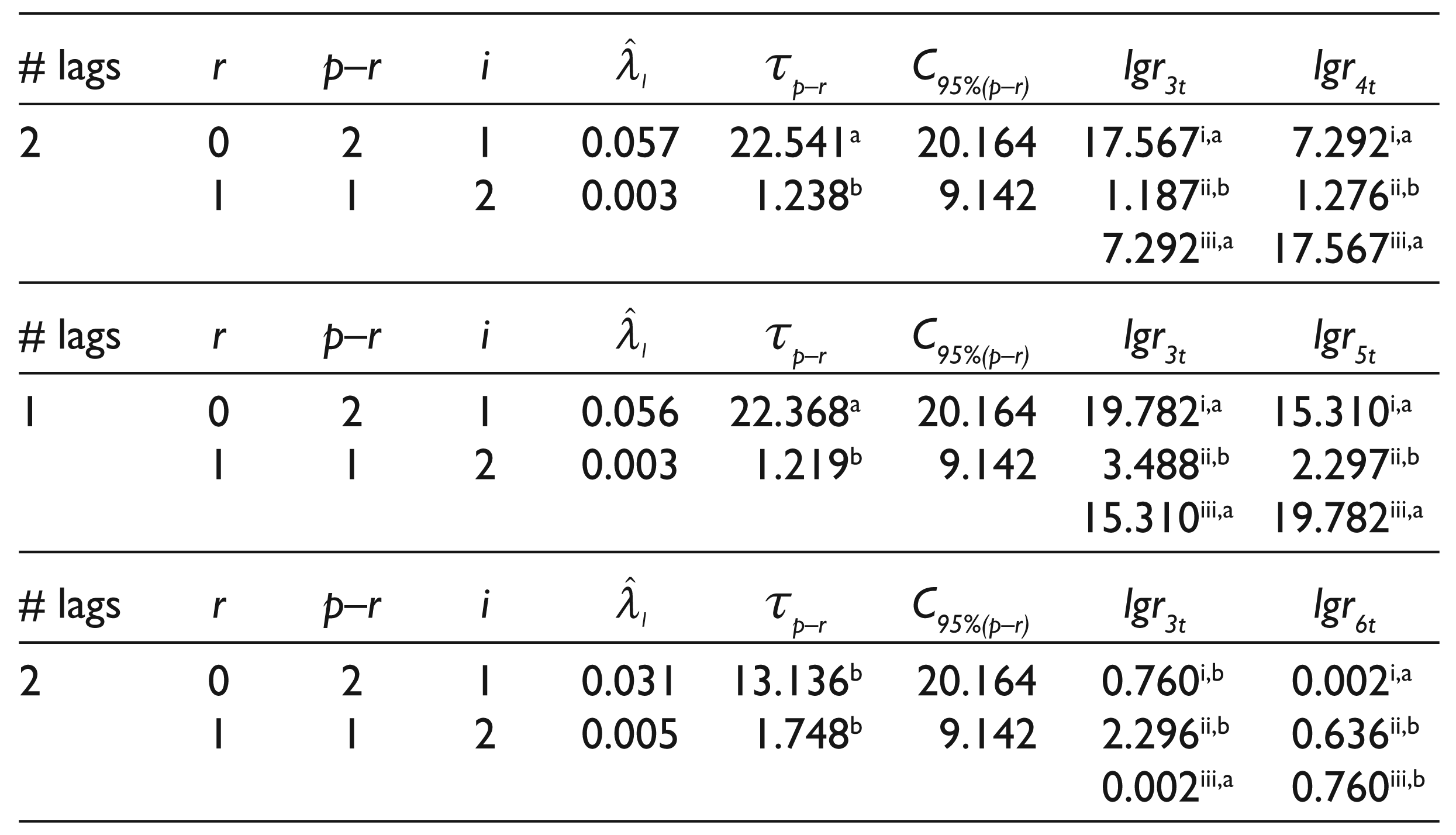
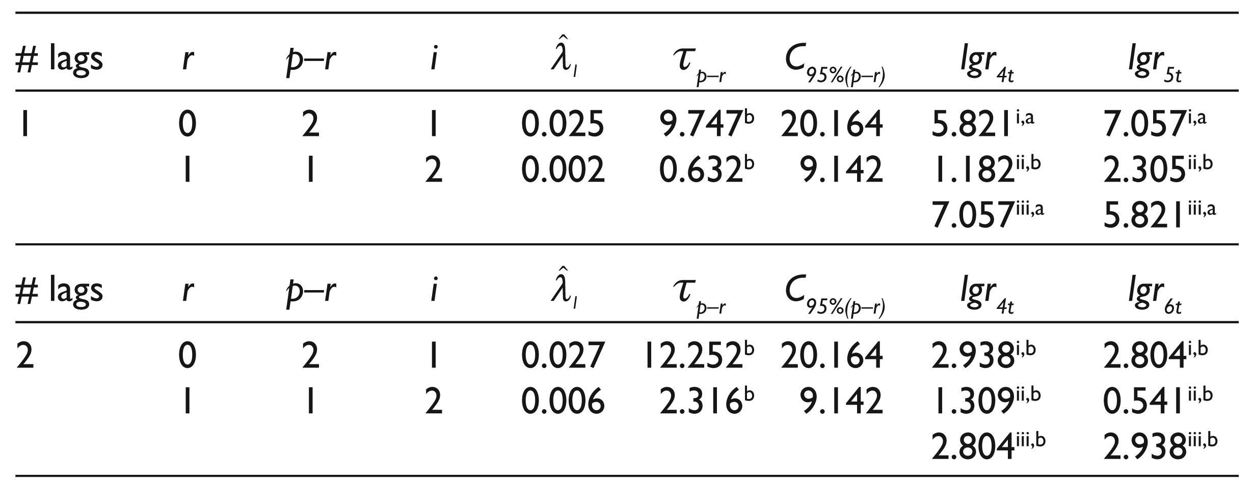
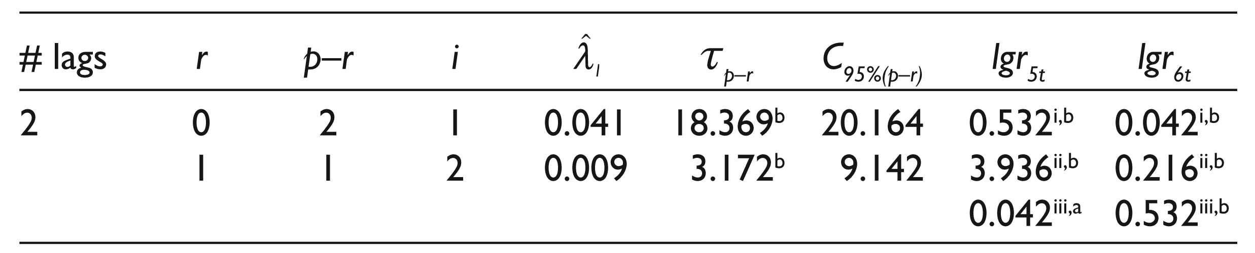
2. ^b Acceptance of the null with 95 per cent significance.

3. ⁱ Multivariate stationarity test is a LR test, distributed as χ ²(1).

4. ⁱⁱ Doornik and Hansen (2008) univariate normality test, distributed as χ ²(2).

5. ⁱⁱⁱ Variable exclusion is a LR test, distributed as χ ²(1).

First, employing models Η₂ and Η₃, given the importance of a zero error correction term, we test the validity of long-run weak exogeneity hypothesis for both shares constituting each pair. Estimated coefficients of the error correction terms represent the short-run speed of adjustment; their magnitude and significance are of great importance regarding the results of our study. If the coefficient of a term is zero, then the error correction does not come from that variable. Considering results reported in Tables 3a and 3b, we cannot reject the hypothesis of long-run weak exogeneity for lgr_4t (EFG Eurobank Ergasias) in pair (a), as well as for lgr_5t (Piraeus Bank) in pair (b). Overall, Cyprus Bank is identified as the adjusting variable in both cases, where we identify EFG Eurobank Ergasias and Piraeus Bank as the pushing forces in pairs (a) and (b), respectively.

Table 3a.

Long-run Identification of Cointegrated Pair: lgr_3t , lgr_4t (Full Sample)

	H₁		H₂		H₃		H₄		H₅
	${\hat{α}}_{3}$	${\hat{β}}_{3}$	${\hat{α}}_{3}$	${\hat{β}}_{3}$	${\hat{α}}_{3}$	${\hat{β}}_{3}$	${\hat{α}}_{3}$	${\hat{β}}_{3}$	${\hat{α}}_{3}$	${\hat{β}}_{3}$
lgr_3t	0.038	−0.406	0	−0.025	−0.015	1	−0.008	1	−0.006	1
	(4.460)	(−5.213)		(−0.071)	(−4.437)		(−1.445)		(−1.140)
lgr_4t	0.001	1	−0.008	1	0	−2.471	−0.005	−1	0	−1
	(0.068)		(−1.690)			(−8.149)	(−1.062)
Constant		−2.057		−2.650		5.088		1.218		1.292
		(−17.750)		(−5.034)		(6.383)		(5.438)		(4.346)
Log likelihood	2,471.244		2,462.123		2,471.242		2,461.842		2,461.310
LR statistic			18.244		0.004		18.806		19.870
p-value			0.000		0.948		0.000		0.000
			χ ²(1)		χ ²(1)		χ ²(1)		χ ²(2)

Source: Datastream.

Note: Numbers in brackets are t -ratios.

Table 3b.

Long-run Identification of Cointegrated Pair: lgr_3t , lgr_5t (Full Sample)

	H₁		H₂		H₃		H₄		H₅
	${\hat{α}}_{4}$	${\hat{β}}_{4}$	${\hat{α}}_{4}$	${\hat{β}}_{4}$	${\hat{α}}_{4}$	${\hat{β}}_{4}$	${\hat{α}}_{4}$	${\hat{β}}_{4}$	${\hat{α}}_{4}$	${\hat{β}}_{4}$
lgr_3t	0.043	−0.801	0	−0.793	−0.029	1	−0.034	1	−0.029	1
	(4.659)	(−10.877)		(−0.752)	(−3.947)		(−3.896)		(−3.296)
lgr_5t	0.014	1	−0.003	1	0	−1.249	−0.012	−1	0	−1
	(1.687)		(−1.028)			(−11.803)	(−1.449)
Constant		−1.195		−1.929		1.518		0.919		0.944
		(−10.810)		(−1.217)		(6.039)		(15.827)		(15.233)
Log likelihood	2,475.173		2,65.237		2,473.835		2,472.050		2,471.087
LR statistic			19.871		2.675		6.246		8.170
p-value			0.000		0.102		0.012		0.017
			χ ²(1)		χ ²(1)		χ ²(1)		χ ²(2)

Source: Datastream.

Note: Numbers in brackets are t -ratios.

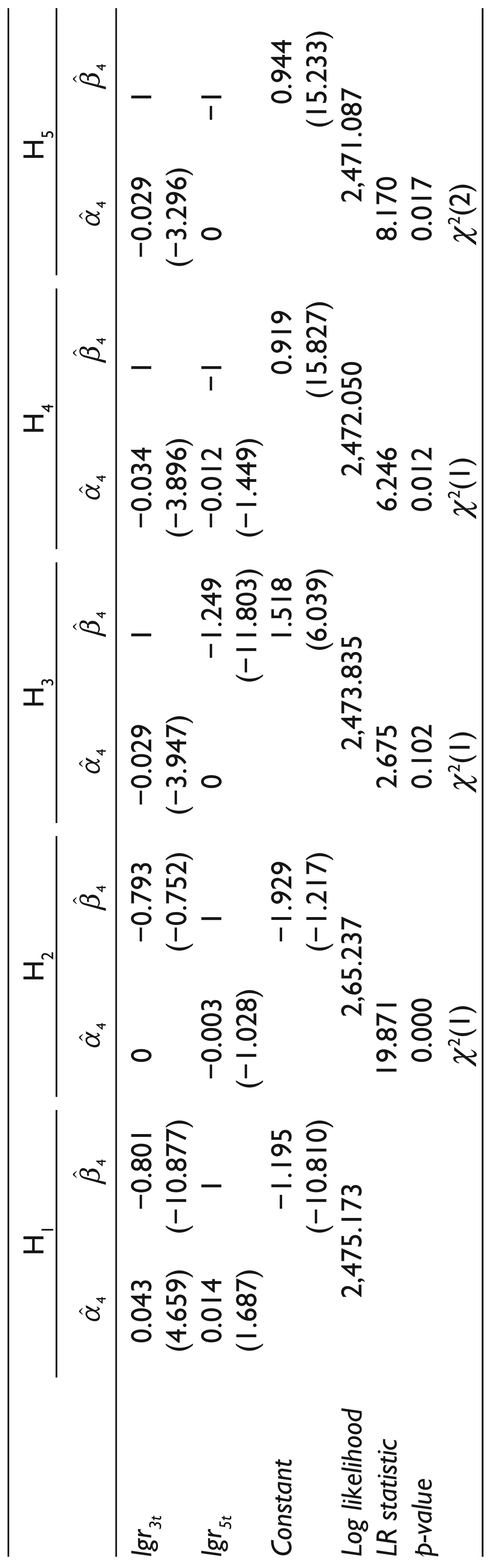
Regarding the second overidentifying restriction, employing model Η₄, we test the null hypothesis of long-run homogeneity between share prices in each pair. Reported results, considering model Η₄ (in Tables 3a and 3b), indicate rejection of long-run homogeneity hypothesis in both pairs [(a) lgr_3t –lgr_4t and (b) lgr_3t –lgr_5t]. Moreover, examining model Η₅, we reject as well the null joint hypothesis of long-run weak exogeneity and long-run homogeneity.

Summing up, we detect two well-established cointegrating relations. The cointegrating relations β₁ , and β₂ , implied by model Η₃ (in Tables 3a and 3b, respectively), are as follows:

β_{1} : \lg r_{3 t} = \underset{(- 6.383)}{- 5.088} + \underset{(8.149)}{2.471} \cdot \lg r_{4 t} + s t a t . e r r o r

(5)

β_{2} : \lg r_{3 t} = \underset{(- 6.039)}{- 1.518} + \underset{(11.803)}{1.249} \cdot \lg r_{5 t} + s t a t . e r r o r

(6)

The previously described cointegrating relations (β₁ , and β₂ ) seem to be stable in the short-run as well, as we can infer from the negative sign and significance of the coefficient corresponding to Δlgr_3t (model H₃, in Tables 3a and 3b, respectively) reported in α matrix. In other words, the share prices of the bank identified as the adjusting process seem to adjust very well to the long-run relations.

In the second empirical part, our analysis is focused on the two pairs [(a) lgr_3t –lgr_4t and (b) lgr_3t –lgr_5t), where well-established cointegrating relations have been detected. Splitting the examined sample into two sub-periods, we perform cointegration tests and hypothesis testing in each subsample. We have employed a model with one lag in the first sub-period and a model with one or two lags in the second sub-period. In order to secure valid statistical inference, we choose to control for the largest of observations by dummy variables. Equation (4) describes the model employed in the two sub-periods.

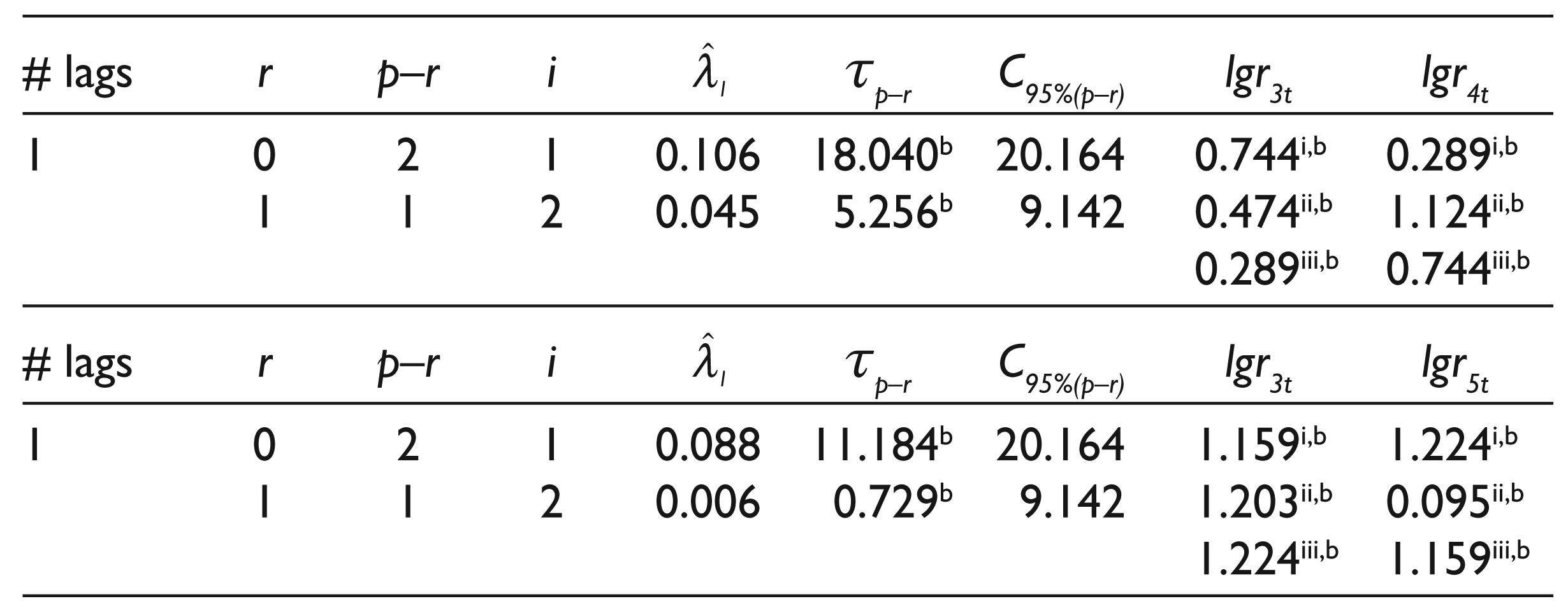
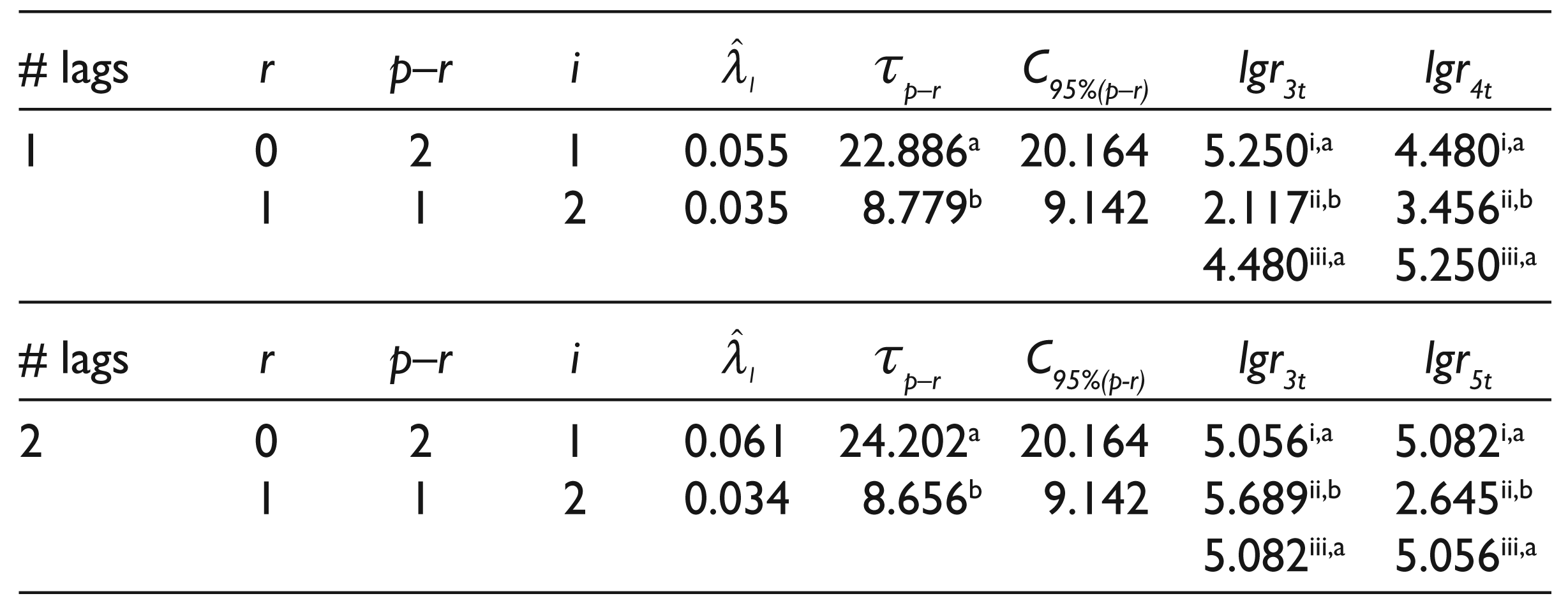
The results, in Table 4, suggest the acceptance of a cointegration rank equal to zero regarding both examined pairs, in the first sub-period. On the other hand, as indicated by the results in Table 5, considering the second sub-period, with 95 per cent significance, the null hypothesis of r = 0 is rejected, while a cointegration rank equal to one is accepted, in both cases.

Table 4.

Bivariate Trace Tests for Cointegration Rank and Hypothesis Testing (First Subsample)

# lags	r	p–r	i	${\hat{λ}}_{l}$	τ_p–r	C_95%(p–r)	lgr_3t	lgr_4t
1	0	2	1	0.106	18.040^b	20.164	0.744^i,b	0.289^i,b
	1	1	2	0.045	5.256^b	9.142	0.474^ii,b	1.124^ii,b
							0.289^iii,b	0.744^iii,b
# lags	r	p–r	i	${\hat{λ}}_{l}$	τ_p–r	C_95%(p–r)	lgr_3t	lgr_5t
1	0	2	1	0.088	11.184^b	20.164	1.159^i,b	1.224^i,b
	1	1	2	0.006	0.729^b	9.142	1.203^ii,b	0.095^ii,b
							1.224^iii,b	1.159^iii,b

Source: Datastream.

Notes: 1. ^a Rejection of the null with 95 per cent significance.

2. ^b Acceptance of the null with 95 per cent significance.

3. ⁱ Multivariate stationarity test is a LR test, distributed as χ ²(1).

4. ⁱⁱ Doornik and Hansen (2008) univariate normality test, distributed as χ ²(2).

5. ⁱⁱⁱ Variable exclusion is a LR test, distributed as χ ²(1).

Table 5.

Bivariate Trace Tests for Cointegration Rank and Hypothesis Testing (Second Subsample)

# lags	r	p–r	i	${\hat{λ}}_{l}$	τ_p–r	C_95%(p–r)	lgr_3t	lgr_4t
1	0	2	1	0.055	22.886^a	20.164	5.250^i,a	4.480^i,a
	1	1	2	0.035	8.779^b	9.142	2.117^ii,b	3.456^ii,b
							4.480^iii,a	5.250^iii,a
# lags	r	p–r	i	${\hat{λ}}_{l}$	τ_p–r	C_95%(p-r)	lgr_3t	lgr_5t
2	0	2	1	0.061	24.202^a	20.164	5.056^i,a	5.082^i,a
	1	1	2	0.034	8.656^b	9.142	5.689^ii,b	2.645^ii,b
							5.082^iii,a	5.056^iii,a

Source: Datastream.

Notes: 1. ^a Rejection of the null with 95 per cent significance.

2. ^b Acceptance of the null with 95 per cent significance.

3. ⁱ Multivariate stationarity test is a LR test, distributed as χ ²(1).

4. ⁱⁱ Doornik and Hansen (2008) univariate normality test, distributed as χ ²(2).

5. ⁱⁱⁱ Variable exclusion is a LR test, distributed as χ ²(1).

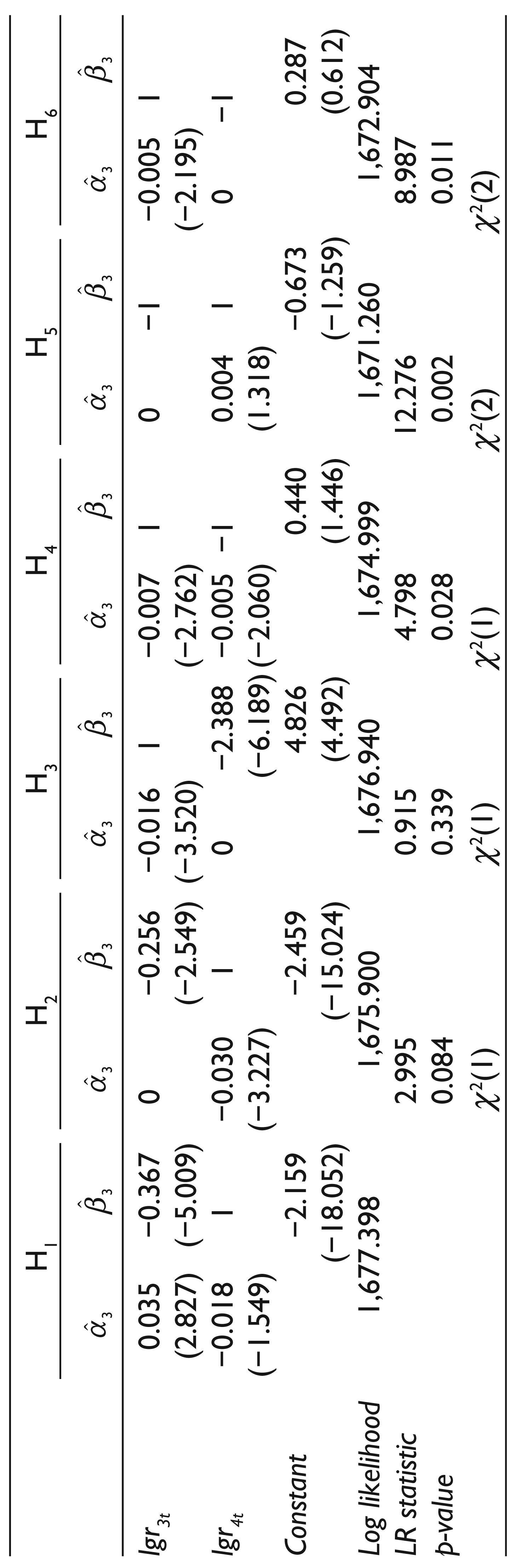
Given the previously mentioned results of cointegration tests, in the third part of our analysis, we focus in the second sub-period in order to perform long-run identification of the two cointegrated pairs. Proceeding in the same line as in the first empirical part, we examine the dynamics of each system, performing hypothesis testing. In Tables 6a and 6b, we begin our analysis with the unrestricted model H₁, normalising the β vector to lgr_4t , in the first case (Table 6a), and to lgr_5t , in the second case (Table 6b). Although normalisation of each cointegrated vector leads to identified cointegrating relations, we choose to impose overidentifying restrictions.

First, given the importance of a zero error correction term, employing models H₂ and H₃, we test the validity of long-run weak exogeneity hypothesis, on both shares constituting each pair. Reported results, in Table 6a, indicate rejection of the hypothesis of long-run weak exogeneity for each of the shares of Cyprus Bank or EFG Eurobank Ergasias. That is, in the case of the first pair (lgr_3t –lgr_4t ), we cannot distinguish between the stochastic trend and the adjusting process of the system. However, in the second pair (lgr_3t –lgr_5t ), reported results, in Table 6b, indicate that we cannot reject the hypothesis of long-run weak exogeneity for Piraeus Bank. Overall, only in the cointegrated relation between Cyprus Bank and Piraeus Bank, we have evidence of a well-established system, where Piraeus Bank is the pushing variable, while Cyprus Bank is purely adjusting.

Table 6a.

Long-run Identification of Cointegrated Pair: lgr ₃t , lgr _4t (Second Subsample)

	H₁		H₂		H₃		H₄		H₅		H₆
	${\hat{α}}_{3}$	${\hat{β}}_{3}$	${\hat{α}}_{3}$	${\hat{β}}_{3}$	${\hat{α}}_{3}$	${\hat{β}}_{3}$	${\hat{α}}_{3}$	${\hat{β}}_{3}$	${\hat{α}}_{3}$	${\hat{β}}_{3}$	${\hat{α}}_{3}$	${\hat{β}}_{3}$
lgr_3t	0.035	−0.367	0	−0.256	−0.016	1	−0.007	1	0	−1	−0.005	1
	(2.827)	(−5.009)		(−2.549)	(−3.520)		(−2.762)				(−2.195)
lgr_4t	−0.018	1	−0.030	1	0	−2.388	−0.005	−1	0.004	1	0	−1
	(−1.549)		(−3.227)			(−6.189)	(−2.060)		(1.318)
Constant		−2.159		−2.459		4.826		0.440		−0.673		0.287
		(−18.052)		(−15.024)		(4.492)		(1.446)		(−1.259)		(0.612)
Log likelihood	1,677.398		1,675.900		1,676.940		1,674.999		1,671.260		1,672.904
LR statistic			2.995		0.915		4.798		12.276		8.987
p-value			0.084		0.339		0.028		0.002		0.011
			χ ²(1)		χ ²(1)		χ ²(1)		χ ²(2)		χ ²(2)

Source: Datastream.

Note: Numbers in brackets are t -ratios.

Table 6b.

Long-run Identification of Cointegrated Pair: lgr_3t , lgr_5t (Second Subsample)

	H₁		H₂		H₃		H₄		H₅
	${\hat{α}}_{4}$	${\hat{β}}_{4}$	${\hat{α}}_{4}$	${\hat{β}}_{4}$	${\hat{α}}_{4}$	${\hat{β}}_{4}$	${\hat{α}}_{4}$	${\hat{β}}_{4}$	${\hat{α}}_{4}$	${\hat{β}}_{4}$
lgr_3t	0.048	−0.757	0	−0.719	−0.036	1	−0.013	1	−0.023	1
	(3.967)	(−10.891)		(−5.989)	(−3.667)		(−3.063)		(−2.605)
lgr_5t	0.010	1	−0.023	1	0	−1.329	−0.010	−1	0	−1
	(0.923)		(−2.777)			(−12.493)	(−2.562)
Constant		−1.260		−1.605		1.733		0.485		0.859
		(−10.968)		(−8.093)		(6.367)		(2.977)		(8.911)
Log likelihood	1,697.594		1,694.212		1,697.402		1,695.656		1,693.667
LR statistic			6.765		0.383		3.877		7.854
p-value			0.009		0.536		0.049		0.020
			χ ²(1)		χ ²(1)		χ ²(1)		χ ²(2)

Source: Datastream.

Note: Numbers in brackets are t -ratios.

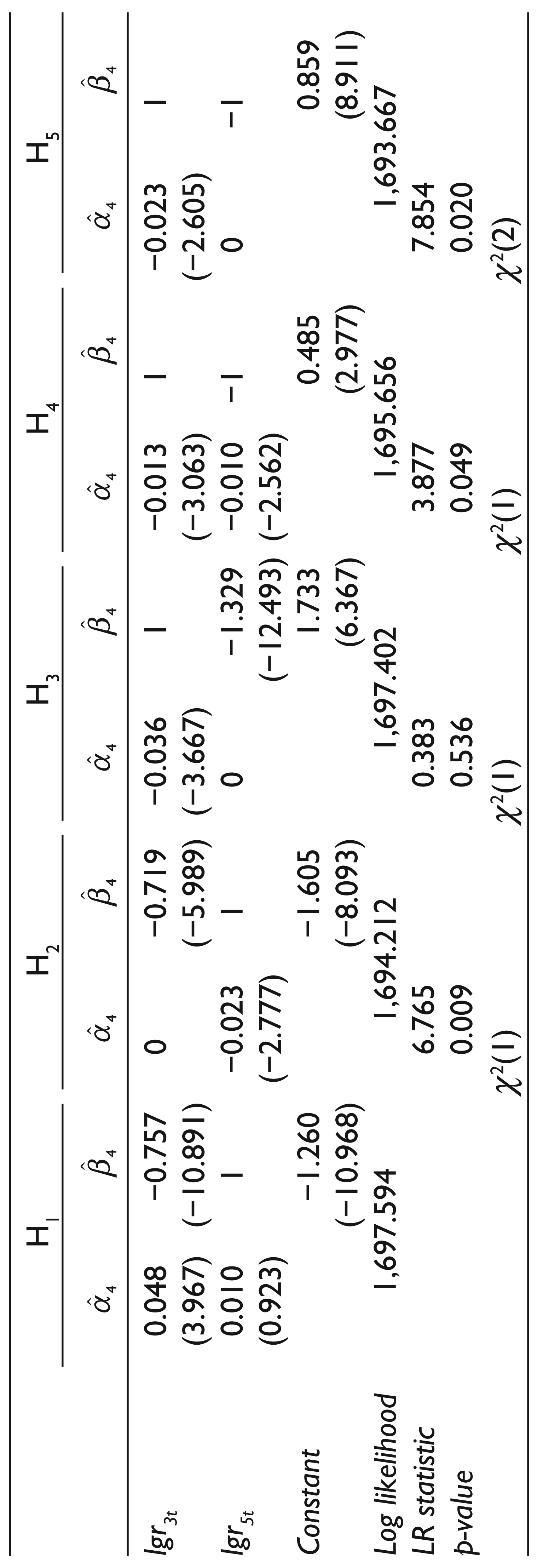
Regarding the second overidentifying restriction, employing model H₄, we test the null hypothesis of long-run homogeneity between the share prices in each pair. Reported results, considering model H₄ (in Tables 6a and 6b), indicate rejection of long-run homogeneity hypothesis in all the examined pairs. Therefore, there is no evidence of a cointegrated vector (1, −1) in any case. Moreover, employing model H₅, in the last case (Table 6b) and examining models H₅ and H₆ in the first case (Table 6a), we reject the null joint hypothesis of long-run weak exogeneity and long-run homogeneity, in all the examined pairs.

Summing up, considering data from the second subsample, we detect just one well-established cointegrating relation. The cointegrating relation β΄₂ , implied by model H₃ (Tables 6b), is described in Equation (7).

{β^{'}}_{2} : \lg r_{3 t} = \underset{(- 6.367)}{- 1.733} + \underset{(12.493)}{1.329} \cdot \lg r_{5 t} + s t a t . e r r o r

(7)

The previously described cointegrating relation, β΄₂ , seems to be stable in the short run as well, as we can infer from the negative sign and significance of the coefficient corresponding to Δlgr_3t (model H₃, in Table 6b), reported in α matrix. In other words, the share prices of Cyprus Bank, identified as the adjusting processes, seem to adjust very well to the long-run relation between Cyprus Bank and Piraeus Bank.

Moreover, the outcome from the ADF (Dickey & Fuller, 1981) unit root test (in Table 7) indicates, with 99 per cent significance, acceptance of the null hypothesis, while points to a stationary spread, with 95 per cent significance.

Table 7.

Augmented Dickey–Fuller Unit Root Test on Spread (Second Subsample)

Spread	# lags	Significance Level			T-statistic
Spread	# lags	99%	95%	90%	T-statistic
lgr_3t–1.329^.lgr_5t	0	−3.458	−2.873	−2.573	−3.302^b,a*

Source: Datastream.

Notes: 1. ^a Rejection of the null with 99 per cent significance.

2. ^b Acceptance of the null with 99 per cent significance.

3. ^a* Rejection of the null with 95 per cent significance.

4. ^b* Acceptance of the null with 95 per cent significance.

5. Summary and Conclusions

Compared with previous research, we extend existing literature by considering pairwise long-run relations between log prices of stocks, under different market conditions. Also, we investigate the implications of these relations on the implementation of SA strategies.

In investigating pairwise long-run relations between banks’ equity shares, quoted in the Greek stock market, we have found two well-established cointegrating relations. Based on that finding, one could set up SA strategies in order to exploit the mean-reverting properties of these two spreads. However, taking into account a structural change due to alternation in market conditions, our results indicate that one should be cautious about applying such strategies. That is, further investigating the long-run relations among the examined stocks, we have divided the sample into two sub-periods in order to re-examine the suggested linear relations under different market conditions.

The examined subsamples contain an intense ‘bear’ phase followed by a moderate ‘bullish’ period. Employing cointegration analysis, reported results initially indicate that changes in market performance affect the stability of long-run relations, suggesting that arbitrageurs should perform rebalancing among the examined equity shares when a change in market trend is evident. Furthermore, intense market performance harms the mean-reverting properties of the two long-run relations while moderate market performance points to cointegration between the examined stocks in each pair. However, under mild market performance, we have found that there is one well-established cointegrating relation that retains the same characteristics shown in the analysis of the examined full sample data.

Declaration of Conflicting Interests

The author(s) declared no potential conflicts of interest with respect to the research, authorship and/or publication of this article.

Funding

The author(s) received no financial support for the research, authorship and/or publication of this article.

Footnotes

Notes

References

Alexakis

(2010). Long-run relations among equity indices under different market conditions: Implications on the implementation of statistical arbitrage strategies. Journal of International Financial Markets, Institutions and Money, 20(4), 389–403.

Alexander

(2001). Market models: A guide to financial data analysis. Chichester: John Wiley & Sons Ltd.

Alexander

, & Dimitriu

(2002). The cointegration alpha: Enhanced index tracking and long-short equity market neutral strategies (ISMA Finance Discussion Paper No. 2002-08). University of Reading, UK: ISMA Centre.

Alexander

, & Dimitriu

(2005). Indexing and statistical arbitrage. Journal of Portfolio Management, 31(2), 50–63.

Bahman

(2013). Stochastic modelling and methods for portfolio management in cointegrated markets (PhD thesis). Oxford: St Anne’s College, University of Oxford.

Balvers

, Wu

, & Gilliland

(2000). Mean reversion across national stock markets and parametric contrarian investment strategies. The Journal of Finance, 55(2), 745–772.

Bhardwaj

R. K.

, & Brooks

L. D.

(1993). Dual betas from bull and bear markets: Reversal of the size effects. The Journal of Financial Research, 6(4), 269–283.

Bondarenko

(2003). Statistical arbitrage and securities prices. The Review of Financial Studies, 16(3), 875–919.

Caldeira

J. F.

, & Moura

G. V.

(2013). Selection of a portfolio of pairs based on cointegration: A statistical arbitrage strategy. Brazilian Review of Finance, 11(1), 49–80.

10.

Canjels

, Prakash-Canjels

, & Taylor

(2004). Measuring market integration: Foreign exchange arbitrage and the gold standard, 1879–1913. The Review of Economics and Statistics, 86(4), 868–882.

11.

Chaudhuri

, & Wu

(2003a). Mean reversion in stock prices: Evidence from emerging markets. Managerial Finance, 29(10), 22–37.

12.

Chaudhuri

, & Wu

(2003b). Random walk versus breaking trend in stock prices: Evidence from emerging markets. Journal of Banking & Finance, 27(4), 575–592.

13.

Cheng

T. Y.

, Lee

C. I.

, & Lin

C. H.

(2013). An examination of the relationship between the disposition effect and gender, age, the trading security, and bull–bear market conditions. Journal of Empirical Finance, 21(1), 195–213.

14.

Choudhry

(1997). Stochastic trends in stock prices: Evidence from Latin American markets. Journal of Macroeconomics, 19(2), 285–304.

15.

Chow

G. C.

(1960). Tests of equality between sets of coefficients in two linear regressions. Econometrica, 28(3), 591–605.

16.

Cuthbertson

(1996). Quantitative financial economics: Stocks, bonds and foreign exchange. Chichester: Wiley.

17.

Dennis

J. G.

, Hansen

, Johansen

, & Juselius

(2005). CATS in RATS, cointegration analysis of time series, version 2. Evanston, Illinois: Estima.

18.

Dickey

D. A.

, & Fuller

W. A.

(1981). Likelihood ratio statistics for autoregressive time series with a unit root. Econometrica, 49(4), 1057–1072.

19.

Doornik

J. A.

, & Hansen

(2008). An omnibus test for univariate and multivariate normality. Oxford Bulletin of Economics and Statistics, 70(s1), 927–939.

20.

Engle

R. F.

, & Granger

C. W. J.

(1987). Cointegration and error correction: Representation, estimation and testing. Econometrica, 55(2), 251–276.

21.

Fabozzi

F. J.

, & Francis

J. C.

(1977). Stability tests for alphas and betas over ‘bull’ and ‘bear’ market conditions. The Journal of Finance, 32(4), 1093–1099.

22.

Fama

E. F.

(1965). The behaviour of stock market price. Journal of Business, 38(1), 34–105.

23.

Fama

E. F.

(1970). Efficient capital markets: A review of the theory and empirical work. The Journal of Finance, 25(2), 383–416.

24.

Fama

E. F.

, & French

K. R.

(1988). Permanent and temporary components of stock prices. Journal of Political Economy, 96(2), 246–273.

25.

Forbes

, Kalb

, & Kofman

(1999). Bayesian arbitrage threshold analysis. Journal of Business & Economic Statistics, 17(3), 364–372.

26.

Gatev

, Goetzmann

W. N.

, & Rouwenhorst

K. G.

(2006). Pairs trading: Performance of a relative-value arbitrage rule. The Review of Financial Studies, 19(3), 797–827.

27.

Gonzalo

(1994). Five alternative methods of estimating long-run equilibrium relationships. Journal of Econometrics, 60(1), 203–233.

28.

Gori

(2009). Inside the risk arbitrage: A global review of pairs trading by quant methods and strategies. Saarbrucken: VDM Verlag Dr. Muller.

29.

Grieb

T. A.

, & Reyes

M. G.

(1999). Random walk tests for Latin American equity indexes and individual firms. Journal of Financial Research, 22(4), 371–383.

30.

Hamilton

J. D.

(1994). Times series analysis. Princeton, NJ: Princeton University Press.

31.

Harasty

, & Roulet

(2000). Modeling stock market returns. Journal of Portfolio Management, 26(2), 33–46.

32.

Hogan

, Jarrow

, Teo

, & Warachka

(2004). Testing market efficiency using statistical arbitrage with applications to momentum and value trading strategies. Journal of Financial Economics, 73(3), 525–565.

33.

Huber

(1997). Stock market returns in thin markets: Evidence from the Vienna stock exchange. Applied Financial Economics, 7(5), 493–498.

34.

Jacobsen

(2008). Demonstrating error-correction modelling for intraday statistical arbitrage. Applied Financial Economics Letters, 4(4), 287–292.

35.

Jansen

D. W.

, & Tsai

C. L.

(2010). Monetary policy and stock returns: Financing constraints and asymmetries in bull and bear markets. Journal of Empirical Finance, 17(5), 981–990.

36.

Johansen

(1988). Statistical analysis of cointegrating vectors. Journal of Economic Dynamics and Control, 12(2, 3), 231–254.

37.

Johansen

(1996). Likelihood-based inference on cointegration in the vector autoregressive model. Oxford: Oxford University Press.

38.

Johansen

, & Juselius

(1990). Maximum likelihood estimation and inference on cointegration with applications to the demand for money. Oxford Bulletin of Economics and Statistics, 52(2), 169–210.

39.

Juselius

(2006). The cointegrated VAR model: Methodology and applications. Oxford: Oxford University Press.

40.

Juselius

, & MacDonald

(2003). International parity relationships between Germany and the United States: A joint modelling approach (Working Paper No. FRU 2004/08). Copenhagen: University of Copenhagen, Department of Economics, Finance Research Unit.

41.

Kawakatsu

, & Morey

M. R.

(1999). An empirical examination of financial liberalisation and the efficiency of the emerging market stock prices. Journal of Financial Research, 22(4), 385–411.

42.

Krauss

(2016). Statistical arbitrage pairs trading strategies: Review and outlook. Journal of Economic Surveys, 31(2), 513–545.

43.

Kremers

J. J.

, Ericsson

N. R.

, & Dolado

J. J.

(1992). The power of cointegration tests. Oxford Bulletin of Economics and Statistics, 54(3), 325–348.

44.

Laopodis

, & Sawhney

(2002). Dynamic interactions between main street and wall street. The Quarterly Review of Economics and Finance, 42(4), 803–815.

45.

Lin

, McCrae

, & Gulati

(2006). Loss protection in pairs trading through minimum profit bounds: A cointegration approach. Journal of Applied Mathematics and Decision Sciences, 2006, 1–14.

46.

Liu

, & Timmermann

(2013). Optimal convergence trade strategies. Review of Financial Studies, 26(4), 1048–1086.

47.

Liu

, Song

, & Romilly

(1997). Are Chinese stock markets efficient? A cointegration and causality analysis. Applied Economics Letters, 4(8), 511–515.

48.

A. W.

, & MacKinlay

A. C.

(1988). Stock market prices do not follow random walks: Evidence from a simple specification test. Review of Financial Studies, 1(1), 41–66.

49.

Marshall

B. R.

, Nguyen

N. H.

, & Visaltanachoti

(2013). ETF arbitrage: Intraday evidence. Journal of Banking and Finance, 37(9), 3486–3498.

50.

Mavrakis

(2011). Abnormal returns on CEFs in pre- and post-credit-crunch periods. European Research Studies, 14(4), 55–70.

51.

Meric

, Ratner

, & Meric

(2008). Co-movement of sector index returns in the world’s major stock markets in bull and bear markets: Portfolio diversification implications. International Review of Financial Analysis, 17(1), 156–177.

52.

Miao

G. J.

(2014). High frequency and dynamic pairs trading based on statistical arbitrage using a two-stage correlation and cointegration approach. International Journal of Economics and Finance, 6(3), 96–110.

53.

Narayan

P. K.

, & Narayan

(2007). Mean reversion in stock prices: New evidence from panel unit root tests. Studies in Economics and Finance, 24(3), 233–244.

54.

Narayan

P. K.

, & Smyth

(2004). Is South Korea’s stock market efficient? Applied Economics Letters, 11(11), 707–710.

55.

Narayan

P. K.

, & Smyth

(2007). Mean reversion versus random walk in G7 stock prices: Evidence from multiple trend break unit root tests. International Financial Markets, Institutions and Money, 17(2), 152–166.

56.

Pole

(2007). Statistical arbitrage: Algorithmic trading insights and techniques. Hoboken, NJ: Wiley.

57.

Poterba

J. M.

, & Summers

L. H.

(1988). Mean reversion in stock prices: Evidence and implications. Journal of Financial Economics, 22(1), 27–59.

58.

Samuelson

(1965). Proof that properly anticipated prices fluctuate randomly. Industrial Management Review, 6(2), 41–49.

59.

Tatom

(2002). Stock prices, inflation and monetary policy. Business Economics, 37(4), 7–19.

60.

Urrutia

J. L.

(1995). Test of random walk and market efficiency for Latin American emerging equity markets. Journal of Financial Research, 18(3), 299–309.

61.

Vidyamurthy

(2004). Pairs trading: Quantitative methods and analysis. Hoboken, NJ: Wiley.

62.

Wang

, & Yau

(1994). A time series approach to testing for market linkage: Unit root and cointegration tests. The Journal of Futures Markets, 14(4), 457–474.

63.

Working

(1960). Note on the correlation of first differences of averages in a random chain. Econometrica, 28(4), 916–918.

64.

Zhu

(1998). The random walk of stock prices: Evidence from a panel of G7 countries. Applied Economics Letters, 5(7), 411–413.