Causality between Cash Flow and Earnings: Evidence from Tehran (Iran) Stock Exchange

Abstract

This article employs data from 155 companies from 27 different industries listed on the Tehran Stock Exchange (TSE) for the period from 2000 to 2009 to examine the direction of causality between cash flow and earnings after taking consideration of stationarity and co-integration. The results indicate that there is a bidirectional causal relationship between cash flow and earnings at the level of all individual companies, so that cash flow variables caused earning variables and vice versa. However, at the level of industrial sectors, causality exists only between earning before interest and taxation (EBIT) and cash flow from operating activities (CFOA).

Keywords

Cash flow earnings Granger causality stationarity co-integration Tehran Stock Exchange Iran

1. Introduction

Both earnings and cash flow are important to companies and shareholders. According to the Trueblood Committee, the objective of income statements and statements of financial activities (cash flow) is to provide useful information for predicting, comparing and evaluating enterprises’ earning power (Wolk, Dodd, & Tearney, 2004). Earnings are the net benefits of a corporation’s operation (Blanc & Setzer, 2015; Eccles, Herz, Keegan, & Philips, 2001). According to the different purposes of accounting activities, several more specific earnings are used, such as earnings before interest and taxation (EBIT) and earnings before interest, taxes, depreciation and amortisation (EBITDA). Cash flow can be defined as the movement of money into or out of the companies, businesses or projects.¹

Different interested parties, such as shareholders, investors or analysts, focus on different aspects of earnings and cash flow. If there is a one-way relationship between cash flow and earnings, it is worthwhile to find out which one is a driver of the other. However, few studies have used econometric models to look into the causality between earnings and cash flow, taking into consideration stationarity and co-integration.

The objective of this study is to explore the causal relationship between cash flows and earnings using the Iranian data, which has not been studied in this context earlier (refer to also Chowdhury, Uddin, & Anderson, 2018, and Tang & Yao, 2018, for discussions on the emerging markets). To ensure that the results are reliable, we test the stationarity and co-integration in the first step. To contribute to the literature, this article uses panel data to control for individual heterogeneity (Baltagi, 2005). This is the first study on such a topic in the Iranian market, which is the largest market in the Middle East in terms of the number of stakeholders, variation of industry and profitability.

The next section provides a review of previous research on cash flow and earnings. The third section describes the models and methodology. The fourth section explains the variables and data collection. The fifth section focuses on the empirical analysis, and the results, discussion and conclusion are presented in the sixth section.

2. Literature Review

So far, previous studies on determining the relationship between cash flow and earnings have not been conclusive. On the one hand, some studies have concluded that ‘earnings’ occupy a central position in accounting in predicting future cash flow for firms. FASB (1978) suggested that earnings provide a better indication than cash flow. However, FASB’s statement did not have empirical support. Greenberg, Johnson and Ramesh (1986) stated that earnings have a greater power of prediction than cash flow. Lorek and Willinger (1996) applied a multivariate, time-series prediction model, and their conclusions were consistent with the viewpoint of FASB that earnings and accrual accounting data can enhance cash flow prediction. Dechow, Kothari and Watts (1998) investigated the ability of current cash flow and earnings to estimate future operating cash flow. They concluded that earnings are a superior predictor than current cash flow and also pointed out that the difference varies with the operating cash cycle. Barth, Cram and Nelson (2001) disaggregated earnings into cash flow and six major accrual parts and found that disaggregated earnings do a better job in predicting future cash flow than current cash flow. Kim and Kross (2005) found that the significance of the relationship between current earnings and future operating cash flow has increased over time. Their conclusion was applicable to different-sized companies with or without paying out dividends.

On the other hand, some researchers have a different view. Bowen, Burgstahler and Daley (1986) used US data and found that net income plus depreciation and amortisation and working capital from operations is the best predictor of cash flow from operation among other four variables. The evidence in the UK (Arnold, Clubb, Mason, & Wearing, 1991) did not support that earnings is a superior predictor than cash flow. Using a large sample, Burgstahler, Jiambalvo and Pyo (1998) concluded that cash flow is a better predictor than aggregated earnings. Krishnan and Largay (2000) found that the direct method of calculating cash flow has a great predictive ability. They concluded that cash flow is superior to earnings in forecasting future cash flow. Seng (2006) examined the predictive ability of earnings and different types of cash flow. The results showed that reported cash flow measures (i.e., CFFO, CFFIA and CFFFA) are better predictors than earnings.

Furthermore, some studies have shown mixed results on the predictive ability of cash flow and earnings. Finger (1994) concluded that earnings or earnings with cash flow are greater predictors of cash flow for most companies. However, cash flow is a better predictor than earnings in the short term. Basu, Lee-Seok and Ching-Lih (1998) found that earnings calculated based on different accounting routines, when used for estimation, have different levels of significance in the prediction of cash flow. Nikkinen and Sahlstrom (2004) stated that the mixed results may be the result of neither cash flow nor aggregated earnings being a good predictor.

Although the econometrics model for causality is frequently used in economic studies (e.g., Aktaş & Yilmaz, 2008; Aqeel & Sabihuddin Butt, 2001; Athanasenas, 2010; Aydemir & Demirhan, 2009; Bowden & Payne, 2009; Calderón & Liu, 2002; Chimobi, 2009; Chiou-Wei, Chen, & Zhu, 2008; Chontanawat, Hunt, & Pierse, 2008; Chowdhury et al., 2018; Gross, 2012; Hurlin & Venet, 2008; Levine, Loaysa, & Beck, 2000; Magnus & Oteng-Abayie, 2008; Payne, 2010), only a few studies in accounting have examined the causality between cash flow and earnings. The empirical work by Bezuidenhout, Mlambo and Hamman (BMH) (2008, 2009) is an exception. Their study has investigated causal relationship between cash flow and earnings of stocks listed on the Johannesburg Stock Exchange using 70 companies from 16 different sectors from 1981 to 2000. They included four types of earnings (EBIT, earning before taxation (EBT), profit after taxation (PAT) and net earnings (EARN)) and compared them to three types of cash flow (cash generated from operations after adjustment for non-cash items (denoted by SUB1), cash generated from operations adjusted for investment income received and working capital (denoted by SUB2) and cash flow from operating activities after adjustments for interest and taxation paid (denoted by SUB3). In their studies, the variables were first tested for stationarity and/or co-integration. Regarding the causal relationship between earnings and cash flow, the authors found that in most cases, cash flow is found to cause earnings when the models are estimated in levels. However, when estimated in first differences, the causal relationship tended to be reversed as earnings cause cash flows. The authors claimed that the results in their study are likely to be affected by data limitations, since the tests used in their study are sensitive to sample sizes. They recommended a follow-up study, whereby panel data should be used.

3. Models and Methodology

Panel Data Regressions

In order to forecast by regression analysis, panel data need to be tested for stationarity and co-integration. Panel data is a pooling of time-series (t) and cross-section (i) data. According to Baltagi (2005), a panel data regression differs from a regular time-series or cross-section regression because it has a double subscript on its variables, that is,

y_{i t} = α + β {X^{'}}_{i t} + u_{i t} i = 1, \dots, N; t = 1, \dots, T

(1)

With i denoting firms and t denoting time, the i subscript therefore denotes the cross-section dimension, whereas t denotes the time-series dimension. α is a scalar, β is K × 1 and X_it is the itth observation on K explanatory variables. Most of the panel data applications utilise a one-way error component model for the disturbances, with

u_{i t} = u_{i} + v_{i t}

(2)

Where μ_i denotes the unobservable individual-specific effect and ν_it denotes the remainder disturbance.

In order to determine causality using an econometric model, the data must be investigated for stationarity and then co-integration.

Stationarity

Most of the econometric models used for forecasting require the underlying time series to be stationary (Gujarati, 2003; Harris & Sollis, 2003), as non-stationary data can lead to spurious results.

The regression Equation 1 can be used to illustrate the concept of ‘stationary’. Based on this definition, panel data are called stationary if μ, σ, cov and ρ remain the same and are constant over time. These conditions guarantee that the behaviour of panel data will identical. In other words, y_it will be stationary if the coefficient of correlation (ρ) is smaller than 1, (0<;ρ<1), and if ρ = 1 means that the equation has a unit root, and in this case, the stationarity provision is abrogated and it is non-stationary.

The unit root test is considered as a more powerful method to test for stationarity (Bezuidenhout et al., 2008; Dickey & Fuller, 1979) and of great assistance in selecting a correct forecasting model (Diebold & Kilian, 1999). According to Baltagi (2005) and Im, Pesaran and Shin (2003), the Im, Pesaran and Shin (IPS) unit root test allows for a heterogeneous coefficient of y_it₋₁ and proposes an alternative testing procedure based on averaging individual unit root test statistics. IPS suggests an average of the ADF tests when u_it is serially correlated with different serial correlation properties across cross-sectional units. Im et al. (2003), in particular, proposed a test based on the average of (augmented) Dickey–Fuller (Dickey & Fuller, 1979) statistics computed for each group in the panel, which they referred to as the t-bar test.

The panel unit root tests by Im et al. (2003) for the panel version of the augmented Dicky–Fuller (ADF) test are based on the following regression:

Δ y_{i t} = α_{i} + ρ_{i} y_{i, t - 1} + η_{i t} + θ_{t} + ε_{i t}

(3)

Where α_i are individual constants, η_it are individual time trends and θ_t are the common time effects. The tests rely on the assumption that E[ε_itε_js] = 0 6 t, s and i → j which is required for calculating common time effects. Thus, if the different series are correlated, the last assumption is violated.

The null hypothesis is that each series in the panel contains a unit root, that is, H ₀ρii

and the alternative hypothesis is that some (but not all) of the individual series have unit roots, that is, H ₁ρi<i, …, N₁ρiiN₁, …, N

Formally, it requires the fraction of the individual time series that are stationary to be nonzero, that is, lim N → 3 (N₁/N) = δ, where 0 < δ ≤ 1. This condition is necessary for the consistency of the panel unit root test. The IPS t-bar statistic is defined as the average of the individual ADF statistics (refer also Baltagi, 2005, p. 242):

\bar{t} = \frac{1}{N} \sum_{i = 1}^{N} t ρ_{i}

where t_ρi is the individual t-statistic for testing H₀: ρi = 0 for all i. In cases where the lag order is always zero (pi = 0 for all i), IPS provide simulated critical values for $\bar{t}$ for different numbers of cross-sections N, series length T and Dickey–Fuller regressions containing intercepts only or intercepts and linear trends. In the general case, where the lag order pi may be nonzero for some cross-sections, IPS show that a properly standardised $\bar{t}$ has an asymptotic N (0,1) distribution.

According to Bezuidenhout et al. (2008), differencing is often used to make the data stationary. Baltagi (2005) recommended that regression models involving non-stationary time series should be estimated in difference form.

Co-integration

Although many time series are non-stationary (having so-called random walk or stochastic trends), it is possible that in the long term, linear combinations of these variables have been stationary during the time (without random walk or stochastic trends). When variables are co-integrated, the regression results may not be spurious and the t- and F-tests are valid (Gujarati, 2003).

The methods for testing for co-integration in panel data have developed very rapidly (refer Pedroni, 1999, 2000, 2001, 2004). One of the most commonly used co-integration testing methods is the residual based panel co-integration test by Pedroni (2004) and Malinen (2011).

To ensure broad applicability of any panel co-integration test, it will be important to allow as much heterogeneity as possible among the individual members of the panel (Pedroni, 2004).

Pedroni (2000, 2004) proposed several tests for the null hypothesis of co-integration in a panel data model, which allows for considerable heterogeneity. Pedroni (2004) suggested two different test statistics for the models with heterogeneous co-integration vectors (Breitung & Pesaran, 2005). Let ${\hat{u}}_{i t} = y_{i t} - {\hat{δ}}^{'}_{i} d_{i t} - {\hat{β}}^{'}_{i} x_{i t}$ denote the OLS residual of the co-integration regression. Pedroni considers two different classes of test statistics: (a) the ‘panel statistic’ that is equivalent to the unit root statistic against homogeneous alternatives, and (b) the ‘Group Mean statistic’ that is analogous to the panel unit root tests against heterogeneous alternatives. The two versions of the t statistic are defined as (refer also Breitung & Pesaran, 2005):

P a n e l z_{p t} = {({\tilde{σ}}_{}^{2}_{N T}^{} \sum_{i = 1}^{N} \sum_{t = 1}^{T} {\hat{u}}_{}^{2}_{i, t - 1}^{})}^{\frac{- 1}{2}} (\sum_{i = 1}^{N} \sum_{t = 1}^{T} {\hat{u}}_{i, t - 1} {\hat{u}}_{i, t} - T \sum_{i = 1}^{N} {\hat{λ}}_{i})

(4)

G r o u p - m e a n_{}^{\tilde{z}}_{p t}^{} = \sum_{i = 1}^{N} {({\hat{σ}}_{i e}^{2} \sum_{t = 1}^{T} {\hat{u}}_{i, t - 1}^{2})}^{\frac{- 1}{2}} (\sum_{t = 1}^{T} {\hat{u}}_{i, t - 1} {\hat{u}}_{i, t} - T {\hat{λ}}_{i})

(5)

where ${\hat{λ}}_{i}$ is a consistent estimator of the one-sided long run variance $λ_{i} = \sum_{j = 1}^{\infty} E (e_{i t} e_{i, t - j}), e_{i t} = u_{i t} - δ_{1} u_{1, t - 1}$ , $δ_{i} = \frac{E (u_{i t} u_{i, t - 1})}{E (u_{i, t - 1}^{2}),} {\hat{α}}_{1 e}^{2}$ denotes the estimated variance of e_it and ${\tilde{σ}}_{}^{2}_{N T}^{} = N^{- 1} \sum_{i = 1}^{N} {\hat{σ}}_{i e}^{2} \cdot$ Pedroni presents values of $μ_{p}, σ_{p}^{2}, a n d \tilde{μ} _{p}, {\tilde{σ}}_{p}^{2}$ such that $\frac{(z_{p t} - μ_{p} \sqrt{N})}{σ_{P}}$ and $\frac{(\tilde{z} _{p t} - \tilde{μ} _{p} \sqrt{N})}{\tilde{σ} _{P}}$ have standard normal limiting distributions under the null hypothesis. The hypotheses to test for co-integration are as follows:

H₀: The variables are not co-integrated.

H₁: The variables are co-integrated.

If H₀ can be rejected in favour of H₁, then it can be concluded that the variables are co-integrated. Otherwise they are not.

Granger Causality

The Granger causality test is used in this study to determine whether causality exists between earnings and cash flows. Within a bivariate context, the Granger-type test states that if a variable x Granger causes variable y, the mean square error (MSE) of a forecast of y based on the past values of both variables is lower than that of a forecast that uses only past values of y (Magnus & Oteng-Abayie, 2008).

Based on definition: one variable is ‘Granger-causes’ (or ‘G-causes’) if a forecast of the second variable based only on its past values is made significantly more accurate by using past values of the first variable. More generally, since the future cannot predict the past, if variable x causes variable y, then changes in x should precede changes in y (Bezuidenhout et al., 2008). In other words, a relationship is causal if an intervention on A can be used to alter B. It can be expressed in this slogan: ‘no cause in, no cause out’ (Hoover, 2006).

According to the econometric model, tests for Granger causality require the variables to be stationary and co-integrated. At each time point, we observe two variables, x_it and y_it, which may have a reciprocal causal relationship.

The initial goal is to formulate a linear model that embodies a reciprocal relationship between x and y. Consider the following set of equations (Bezuidenhout et al., 2008):

\begin{matrix} Y_{i t} = α_{0} + α_{1} y_{1 (t - 1)} + \dots + α_{l} y_{i (t - l ​)} + β_{1} X_{1 (t - 1)} + β_{2} X_{2 (t - 2)} \\ + \dots + β_{l} x_{i (t - l ​)} + ε_{i t} \end{matrix}

(6)

\begin{matrix} x_{i t} = α_{0} + α_{1} x_{1 (t - 1)} + \dots + α_{l} x_{i (t - l ​)} + β_{1} y_{1 (t - 1)} + β_{2} y_{2 (t - 2)} + \dots \\ + β_{l} y_{i (t - l ​)} + ν_{i t} \end{matrix}

(7)

The reported F-statistics are the Wald statistics for the following null and alternative hypotheses:

H_{0} : β_{1} = β_{1} = \dots = β_{l} = 0

H_{1} : a t l e a s t o n e β_{i} i s \neq 0

The null hypothesis is that x does not Granger cause y in the first regression and that y does not Granger cause x in the second regression against the alternative that one variable Granger causes the other.

4. Data and Variables

The Tehran Stock Exchange (TSE) opened in February 1967, with only six companies listed during its first year of trading. Then Government bonds and certain state-backed certificates were traded in the market. The TSE has come a long way since then: today it has evolved into an exciting and growing marketplace where individual and institutional investors trade securities of over 420 companies.² The TSE is now the largest market in the Middle East in terms of the number of stakeholders, variation of industry and profitability.

From the year 2000, the Accounting Standards of Iran (ASI) were officially published and became compulsory for listed companies in Stock Exchanges in Iran. In addition, it is necessary to comply with International Financial Reporting Standards (IFRS), simultaneously. The initial sample includes all listed and delisted common corporations in the TSE.

The period of study is the years 2000 to 2009 (a nine-year period, as the statement of cash flow based on ASI is provided on the basis of five parts from year 2000 (refer Panel B in Table 1). The final sample is decided by applying the following two conditions: (a) corporations whose financial statements have been presented to the TSE for the period of the test and (b) because in pooled financial statements, negative items are neutralised by positive items, data have been selected for non-pooled statements. To meet these two conditions, 155 firms from 27 industries qualified for testing in the final sample.

Table 1.

Adjusted Income Statement and Statement of Cash Flow

PANEL A: Income Statement (denoted by X)
Sales Less: Cost of sales Gross profit Administration and selling expenses Profit before interest and taxation Less: Interest expense Plus: Investment income received Profit before taxation Less: Taxation Earnings	X₁ = EBIT X₂ = EBT X₃ = EARN
PANEL B: Statement of Cash Flow (denoted by Y)
Cash Flow from Operating Activities: EBIT ± Adjusted for non-cash items Cash Flow from Operating Activities: ± Investment income received and Interest paid Cash Flow after Investment Income Received and Interest Paid: Taxation paid Cash Flow after Taxation: Cash Flow from Investment Activities Cash Flow from Financing Activities Net cash	Y₁ = CFOA Y₂ = CFII Y₃ = CFT

Source: Appendix of Accounting Standards of Iran (ASI) number 2 (translated) and International Accounting Standards (IAS) 7, as adjusted.

Note: This table provides a sample of income statement in Panel A and cash flow statement in Panel B.

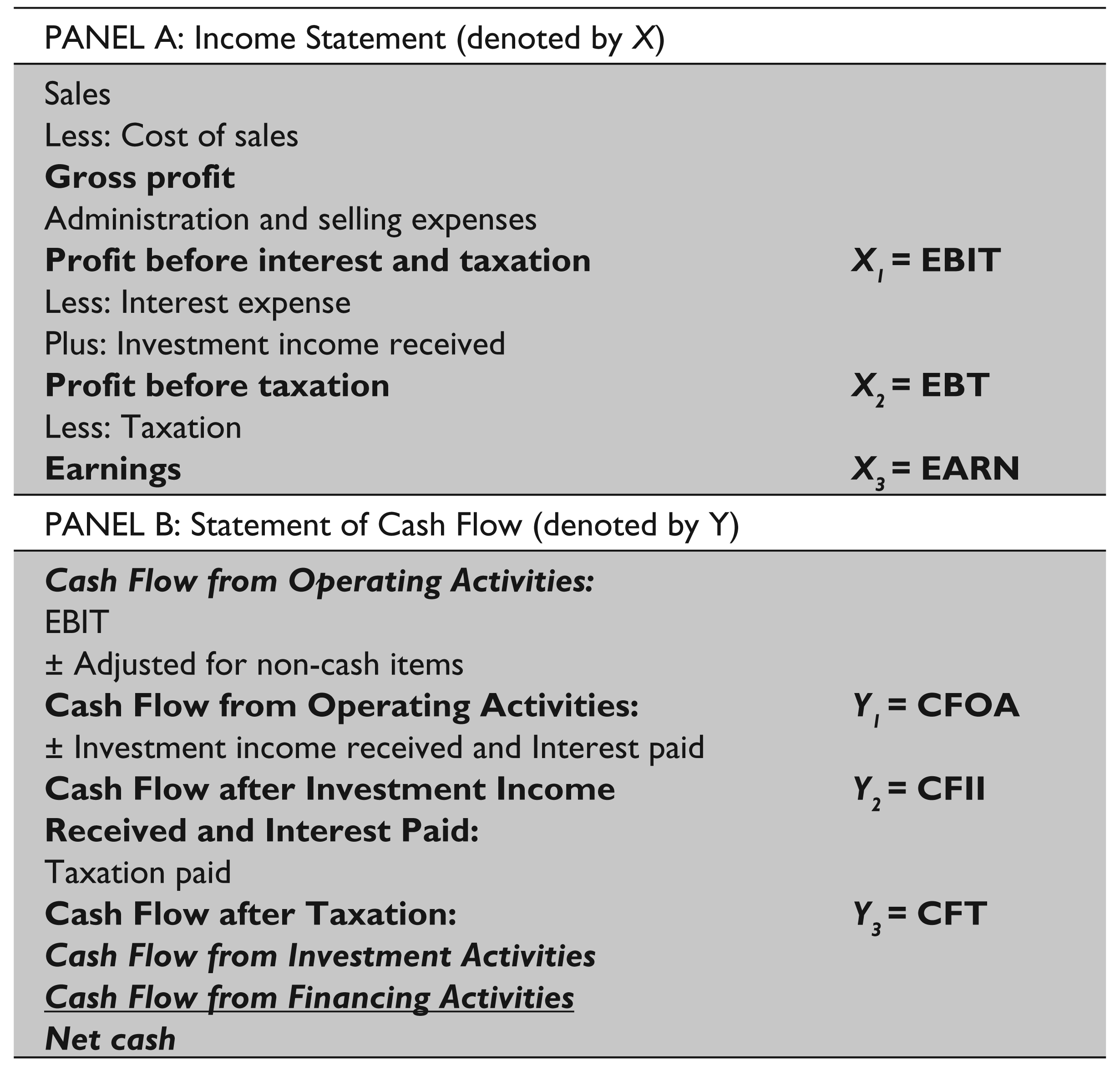
A sample of income and cash flow statements in compliance to ASI and IFRS can be seen in Table 1. While the statement of cash flow for IFRS has three parts, it has five parts based on ASI (refer panel B in Table 1).

Following Bezuidenhout et al. (2008), three variables from income statements (EBIT, EBT and EARN) and three variables from statements of cash flow (CFOA, cash flow after investment income received and interest paid (CFII) and cash flow after taxation (CFT)) (Panel A and B, respectively) are selected for the test, as shown in Table 1.

Data Analysis

Results for data analysis are presented in the following three sections, including test results for stationarity, co-integration and causality, respectively.

Results for Stationarity

To test for causal relationships, the variables need to test for stationarity first. The Im, Pesaran and Shin unit root test results for stationarity is shown in Table 2. The results show that EBIT, denoted by X₁, EBT denoted by X₂, and EARN, denoted by X₃, are non-stationary.

In the statement of cash flow (denoted by Y), with the exception of CFOA denoted by Y₁, the other two variables—CFII denoted by Y₂ and CFT denoted by Y₃—are stationary.

Table 2.

Unit Root Test for Stationary: IM, Pesaran and Shin Model

	p-value	Results
X₁ = EBIT	0.9870	non-stationary
X₂ = EBT	0.9947	non-stationary
X₃ = EARN	0.9884	non-stationary
Y₁ = CFOA	0.1915	non-stationary
Y₂ = CFII	0.0003	stationary
Y₃ = CFT	0.0000	stationary

Source: Authors’ own.

Notes: This table provides Im, Pesaran and Shin unit root test results for stationarity. Earning Before Interest and Taxation (EBIT) is denoted by X₁; Earning Before Taxation (EBT) is denoted by X₂; Earnings (EARN) is denoted by X_3; Operating Activities (CFOA) is denoted by Y₁; Cash Flow after Investment Income Received and Interest Paid (CFII) is denoted by Y₂; and Cash Flow after Taxation (CFT) is denoted by Y_3.

Because the variables X₁, X₂, X₃ and Y₁ have unit roots (are non-stationary), we must test for the existence of long-term relationships among the variables by using a co-integration test.

Results for Co-integration

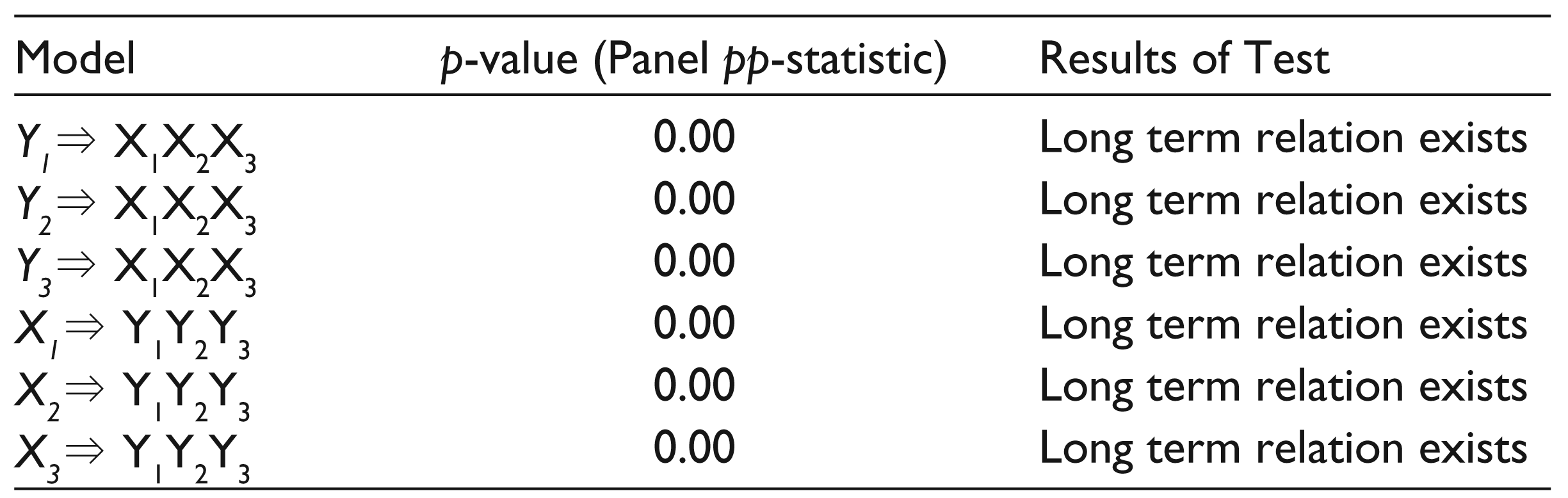
The results for testing co-integration are presented in Table 3. Pedroni’s co-integration test with intercept shows the existence of long-term relationships among the six models. Because of the existence of long-term relationships, it is not necessary to use differencing (refer Baltagi, 2005; Gujarati, 2003; Hendry & Juselius, 2001; 2001; Yini, 2009). It means that panel data are co-integrated (i.e., they have no random walk or stochastic trends).

The null hypothesis, in this test, is a lack of long-term relationships between variables. As presented in Table 3, the p-value is zero, which means that the null hypothesis is rejected. In other words, long-term relationships exist among variables of the model. This makes it possible to investigate for causality among variables.

Results for Causality

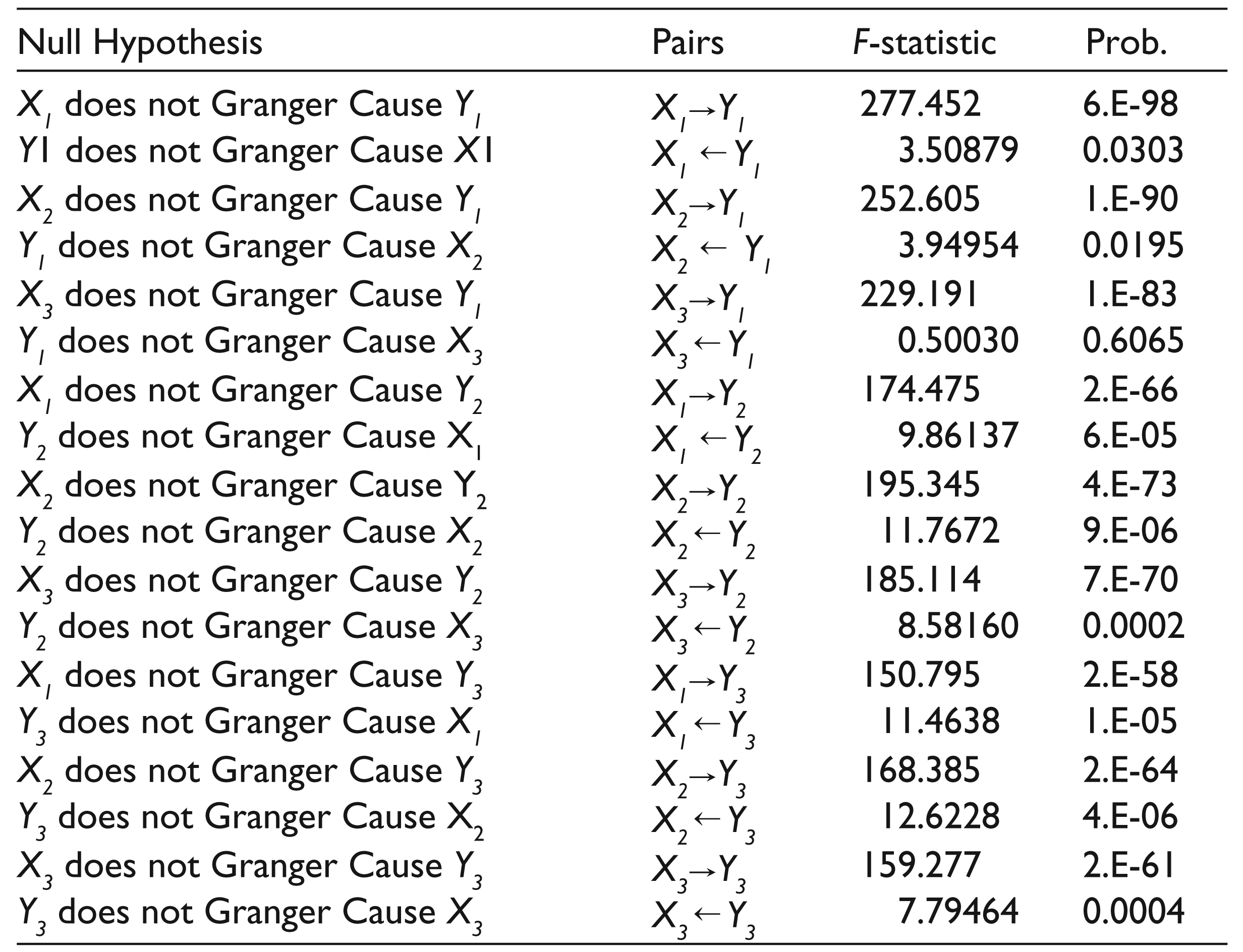
The results of the Granger causality test for all individual companies are given in Table 4. All nine pairs were tested for causality, using the AR models as represented by Equations 6 and 7 in the third section. In all of these nine pairs of variables, cash flow variables were found to cause earnings variables and this relationship was two-way (earning ↔ cash flow). In other words, the results for causality indicate that all nine pairs of variables (for the companies) were causally related and that the causality was bidirectional (two-way).

Table 3.

Results of Pedroni Co-integration Test

Model	p-value (Panel pp-statistic)	Results of Test
Y₁ ⇒ X₁X₂X₃	0.00	Long term relation exists
Y₂ ⇒ X₁X₂X₃	0.00	Long term relation exists
Y₃ ⇒ X₁X₂X₃	0.00	Long term relation exists
X₁ ⇒ Y₁Y₂Y₃	0.00	Long term relation exists
X₂ ⇒ Y₁Y₂Y₃	0.00	Long term relation exists
X₃ ⇒ Y₁Y₂Y₃	0.00	Long term relation exists

Source: Authors’ own.

Notes: this table provides the results from the Pedroni co-integration test with intercept. EBIT is denoted by X₁; EBT is denoted by X₂; EARN is denoted by X_3; CFOA is denoted by Y₁; CFII is denoted by Y₂; and CFT is denoted by Y₃_.

Table 4.

Results for Granger Causality Test from Level of All Companies

Null Hypothesis	Pairs	F-statistic	Prob.
X₁ does not Granger Cause Y₁ Y1 does not Granger Cause X1	X₁ → Y₁ X₁ ← Y₁	277.452 3.50879	6.E-98 0.0303
X₂ does not Granger Cause Y₁ Y₁ does not Granger Cause X₂	X₂ → Y₁ X₂ ← Y₁	252.605 3.94954	1.E-90 0.0195
X₃ does not Granger Cause Y₁ Y₁ does not Granger Cause X₃	X₃ → Y₁ X₃ ← Y₁	229.191 0.50030	1.E-83 0.6065
X₁ does not Granger Cause Y₂ Y₂ does not Granger Cause X₁	X₁ → Y₂ X₁ ← Y₂	174.475 9.86137	2.E-66 6.E-05
X₂ does not Granger Cause Y₂ Y₂ does not Granger Cause X₂	X₂ → Y₂ X₂ ← Y₂	195.345 11.7672	4.E-73 9.E-06
X₃ does not Granger Cause Y₂ Y₂ does not Granger Cause X₃	X₃ → Y₂ X₃ ← Y₂	185.114 8.58160	7.E-70 0.0002
X₁ does not Granger Cause Y₃ Y₃ does not Granger Cause X₁	X₁ → Y₃ X₁ ← Y₃	150.795 11.4638	2.E-58 1.E-05
X₂ does not Granger Cause Y₃ Y₃ does not Granger Cause X₂	X₂ → Y₃ X₂ ← Y₃	168.385 12.6228	2.E-64 4.E-06
X₃ does not Granger Cause Y₃ Y₃ does not Granger Cause X₃	X₃ → Y₃ X₃ ← Y₃	159.277 7.79464	2.E-61 0.0004

Source: Authors’ own.

Notes: this table provides the results of the Granger causality test for all individual companies. EBIT is denoted by X₁; EBT is denoted by X₂; EARN is denoted by X_3; CFOA is denoted by Y₁; CFII is denoted by Y₂; and CFT is denoted by Y_3.

Because causality exists between cash flow and earnings, we can estimate the following equations:

Y_{1 i t} = α + β X_{1 i t} + γ X_{2 i t} + δ X_{3 i t} + ε_{i t}

(8)

Y_{2 i t} = α + β X_{1 i t} + γ X_{2 i t} + δ X_{3 i t} + ε_{i t}

(9)

Y_{3 i t} = α + β X_{1 i t} + γ X_{2 i t} + δ X_{3 i t} + ε_{i t}

(10)

X_{1 i t} = α + β Y_{1 i t} + γ Y_{2 i t} + δ Y_{3 i t} + ε_{i t}

(11)

X_{2 i t} = α + β Y_{1 i t} + γ Y_{2 i t} + δ Y_{3 i t} + ε_{i t}

(12)

X_{3 i t} = α + β Y_{1 i t} + γ Y_{2 i t} + δ Y_{3 i t} + ε_{i t}

(13)

Where Y₁, Y₂, Y₃ denote CFOA, CFII, CFT and X₁, X₂, X₃ denote EBIT, EBT and EARN, respectively.

These equations can be used for forecasting, as we can estimate Y₁ by X₁, X₂ and X₃. Also, conversely, we can estimate X₁ by Y₁, Y₂ and Y₃. This applies to all variables in this test.

Table 5.

Results for Granger Causality Test from Level of Industry Sectors

Null Hypothesis	Pairs	F-statistic	Prob.
X₁ does not Granger Cause Y₁ Y₁ does not Granger Cause X₁	X₁ → Y₁ X₁ ← Y₁	5.61036 6.15772	0.0122 0.0087
X₂ does not Granger Cause Y₁ Y₁ does not Granger Cause X₂	X₂ → Y₁ X₂ ← Y₁	1.80208 1.93071	0.1920 0.1725
X₃ does not Granger Cause Y₁ Y₁ does not Granger Cause X₃	X₃ → Y₁ X₃ ← Y₁	2.40266 2.50517	0.1174 0.1082
X₁ does not Granger Cause Y₂ Y₂ does not Granger Cause X₁	X₁ → Y₂ X₁ ← Y₂	1.25101 1.18497	0.3087 0.3274
X₂ does not Granger Cause Y₂ Y₂ does not Granger Cause X₂	X₂ → Y₂ X₂ ← Y₂	0.85153 1.00478	0.4424 0.3848
X₃ does not Granger Cause Y₂ Y₂ does not Granger Cause X₃	X₃ → Y₂ X₃ ← Y₂	1.23045 1.46277	0.3144 0.2565
X₁ does not Granger Cause Y₃ Y₃ does not Granger Cause X₁	X₁ → Y₃ X₁ ← Y₃	0.91482 0.85918	0.4175 0.4393
X₂ does not Granger Cause Y₃ Y₃ does not Granger Cause X₂	X₂ → Y₃ X₂ ← Y₃	0.64848 0.72467	0.5340 0.4974
X₃ does not Granger Cause Y₃ Y₃ does not Granger Cause X₃	X₃ → Y₃ X₃ ← Y₃	0.95233 1.07921	0.4035 0.3598

Source: Authors’ own.

Notes: this table provides the results for level of industry sectors of the Granger causality test. EBIT is denoted by X₁; EBT is denoted by X₂; EARN is denoted by X_3; CFOA is denoted by Y₁; CFII is denoted by Y₂; CFT is denoted by Y_3.

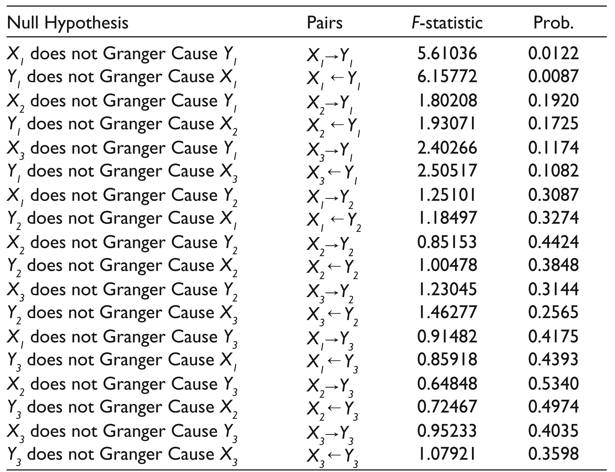
We also test causality for the level of industry sectors. Results from the Granger test are presented in Table 5 for 27 industry sectors. According to the results, causality was only found between variables X₁ and Y₁. In other words, EBIT, denoted by X₁, was caused by CFOA, denoted by Y₁, and vice versa. In other variables, causality was not found.

Discussion and Conclusions

To test for causality between earnings and cash flow, we have investigated stationarity and co-integration. The Im, Pesaran and Shin test is used to investigate stationarity. The Pedroni test is used to investigate co-integration or long-term relationships.

In determining causality for all individual companies, the results show that there are bidirectional relations in all six variables. In other words, all income statement variables have Granger cause (G-cause) on all statements of cash flow and vice versa. For example, EBIT (denoted by X₁) is a Granger cause of CFOA (denoted by Y₁) and vice versa. This means that EBIT can forecast CFOA and that CFOA can forecast EBIT. This bidirectional relationship exists between all pairs of variables X and Y (X↔Y).

As noted in literature review, Bezuidenhout et al. (2008) selected four variables from income statements and three variables from statements of cash flow, using time series analysis. In some conditions, they found bidirectional relations between earnings variables and cash flow variables.

In comparison, we use panel data to investigate causality between variables. Panel data give unbiased and compatible estimations in comparison to time-series data. As noted by Baltagi (2005), panel data give more informative data, more variability, less collinearity among the variables, more degrees of freedom, greater efficiency, and so on. Our panel data includes 155 companies, while the BMH study has 70. According to Bezuidenhout et al. (2008), because of sensitivity to sample sizes, large sample sizes are required if conclusive results are to be reached. As noted by BMH, the size of the sample has an effect on the result of research. We conclude that for individual companies, causality exists between variables of earnings and variables from cash flow, but at the industry level, this bidirectional relationship exists only between EBIT (EBIT = X₁) and CFOA (CFOA = Y₁).

In this study, panel data have more explanatory power and we find that it is better to include more companies. Therefore, we propose that researchers test causal relations in future by using panel data and by increasing the sample size.

Declaration of Conflicting Interests

The author(s) declared no potential conflicts of interest with respect to the research, authorship and/or publication of this article.

Funding

The author(s) received no financial support for the research, authorship and/or publication of this article.

Footnotes

Notes

References

Aktaş

, & Yilmaz

(2008). Causal relationship between oil consumption and economic growth in Turkey. Kocaeli Üniversitesi Sosyal Bilimler Enstitüsü Dergisi, 15(1), 45–55.

Aqeel

, & Sabihuddin Butt

(2001). The relationship between energy consumption and economic growth in Pakistan. Asia-Pacific Development Journal, 8(2), 101–110.

Arnold

A. J.

, Clubb

C. D. B.

, Mason

, & Wearing

R. T.

(1991). The relationship between earnings, funds flows and cash flows: Evidence for the UK. Accounting and Business Research, 22(85), 13–19.

Athanasenas

A. L.

(2010). Credit, income, and causality: A contemporary co-integration analysis. European Journal of Operational Research, 201(1), 194–205.

Aydemir

, & Demirhan

(2009). The relationship between stock prices and exchange rates: Evidence from Turkey. International Research Journal of Finance and Economics, 23, 207–215.

Baltagi

H. B.

(2005). Econometric analysis of panel data (3rd ed.). Chichester: John Wiley & Sons Ltd Publishing Inc.

Barth

M. E.

, Cram

D. P.

, & Nelson

K. K.

(2001). Accruals and the prediction of future cash flows. Accounting Review, 76(1), 27–58.

Basu

, Lee-Seok

, & Ching-Lih

(1998). International variation in accounting measurement rules and analysis earnings forecast errors. Journal for Business Finance and Accounting, 25(9, 10), 1207–1247.

Bezuidenhout

, Mlamboand

, & Hamman

W. D.

(2008). Investigating causality between cash flow and profitability: An econometrics approach. Journal of Meditari Accountancy Research, 16(1), 27–41.

10.

Bezuidenhout

, Mlamboand

, & Hamman

W. D.

(2009). Cash or earnings: Which comes first? University of Stellenbosch Business School (USB). USB LEADERS’ LAB February 2009. Retrieved from www.usb.ac.za/Media/thoughtleadership/leaderslab

11.

Blanc

S. M.

, & Setzer

(2015). Analytical debiasing of corporate cash flow forecasts. European Journal of Operational Research, 243(3), 1004–1015.

12.

Bowden

, & Payne

J. E.

(2009). The causal relationship between U.S. energy consumption and real output: A disaggregated analysis. Journal of Policy Modeling, 31(2), 180–188.

13.

Bowen

R. M.

, Burgstahler

, & Daley

L. A.

(1986). Evidence on relationships between earnings and various measures of cash flow. The Accounting Review, 61(4), 713–725.

14.

Breitung

, & Pesaran

M. H.

(2005). Unit roots and cointegration in panels (Deutsche Bundesbank, Discussion Paper No. 2005, 42, Series 1: Economic Studies). Retrieved from https://ssrn.com/abstract=2785225

15.

Burgstahler

, Jiambalvo

, & Pyo

(1998). The informativeness of cash flows for future cash flows (Working Paper). Seattle, WA: University of Washington.

16.

Calderón

, & Liu

(2002). The direction of causality between financial development and economic growth (Working Papers of the Central bank of Chile, Chile, No. 184, October 2002). Central Bank of Chile.

17.

Chimobi

O. P.

(2009). Government expenditure and national income: A causality test for Nigeria. European Journal of Economic and Political Studies, 2(2), 1–11.

18.

Chiou-Wei

, Chen

, & Zhu

(2008). Economic growth and energy consumption revisited. Evidence from linear and nonlinear Granger causality. Energy Economics, 30(6), 3063–3076.

19.

Chontanawat

, Hunt

, & Pierse

(2008). Does energy consumption cause economic growth? Evidence from a systematic study of over 100 countries. Journal of Policy Modeling, 30(2), 209–220.

20.

Chowdhury

, Uddin

, & Anderson

(2018). Liquidity and macroeconomic management in emerging markets. Emerging Markets Review, 34, 1–24.

21.

Dechow

P. M.

, Kothari

S. P.

, & Watts

R. L.

(1998). The relation between earnings and cash flows. Journal of Accounting and Economics, 25(2), 133–168.

22.

Dickey

D. A.

, & Fuller

W. A.

(1979). Distribution of estimators for autoregressive time series with a unit root. Journal of the American Statistical Association, 74(366), 427–431.

23.

Diebold

F. X.

, & Kilian

(1999). Unit root tests are useful for selecting forecasting models. Retrieved from http://www.ssc.upenn.edu/~diebold

24.

Eccles

R. G.

, Herz

R. H.

, Keegan

E. M.

, & Philips

D. M.

(2001). Revolution: Moving beyond the earnings game. New York, NY: John Wiley and Sons.

25.

FASB (1978). Objectives of financial reporting of business enterprises (Statement of Financial Accounting Concepts No. 1). United States, Norwalk, CT: FASB.

26.

Finger

C. A.

(1994). The ability of earnings to predict future earnings and cash flow. Journal of Accounting Research, 32(2), 210–223.

27.

Greenberg

R. R.

, Johnson

G. L.

, & Ramesh

(1986). Earnings versus cash flow as a predictor of future cash flow measures. Journal of Accounting, Auditing and Finance, 1(4), 266–277.

28.

Gross

(2012). Explaining the (non-) causality between energy and economic growth in the U.S.: A multivariate sectoral analysis. Energy Economics, 34(2), 489–499.

29.

Gujarati

D. N.

(2003). Basic econometrics (4th ed.). New York, NY: McGraw-Hill/Irwin.

30.

Harris

R. I. D.

, & Sollis

(2003). Applied time series modeling and forecasting. West Sussex: Wiley.

31.

Hendry

D. F.

, & Juselius

(2000). Explaining cointegration analysis: Part I. Energy Journal, 21(1), 1–42.

32.

Hendry

D. F.

, & Juselius

(2001). Explaining cointegration analysis: Part II. Energy Journal, 22(1), 75–120.

33.

Hoover

D. K.

(2006). Economic theory and causal inference. Departments of Economics and Philosophy, September, Department of Economics Duke University. Retrieved from http://ssrn.com/abstract=930741

34.

Hurlin

, & Venet

(2008). Financial development and growth: A reexamination using a panel granger causality test. Orléans, France: University of Orleans (Mimeo).

35.

K. S.

, Pesaran

M. H.

, & Shin

(2003). Testing for unit roots in heterogeneous panels. Journal of Econometrics, 115(1), 53–74.

36.

Kim

, & Kross

(2005). The ability of earnings to predict future operating cash flow has been increasing: Not decreasing. Journal of Accounting Research, 43(5), 753–780.

37.

Krishnan

G. V.

, & Largay

J. A.

(2000). The predictive ability of direct method cash flow information. Journal of Business Finance and Accounting, 27(1, 2), 215–245.

38.

Lorek

K. S.

, & Willinger

G. L.

(1996). A multivariate time-series prediction model for cash-flow data. Accounting Review, 71(1), 81–101.

39.

Levine

, Loaysa

, & Beck

(2000). Financial intermediation and growth: Causality and causes. Journal of Monetary Economics, 46(1), 31–77.

40.

Magnus

F. J.

, & Oteng-Abayie

E. F.

(2008). Bivariate causality analysis between FDI inflows and economic growth in Ghana. International Research Journal of Finance and Economics, (15), 1450–2887. Retrieved from https://mpra.ub.uni-muenchen.de/351/1/MPRA_paper_351.pdf

41.

Malinen

(2011). Income inequality and savings: A reassessment of the relationship in cointegrated panels (Discussion Paper No. 337). DEGIT Conference Papers c016_076, DEGIT, Dynamics, Economic Growth, and International Trade. Helsinki Center of Economic Research (HECER).

42.

Nikkinen

, & Sahlstrom

(2004). Impact of an accounting environment on cash flow prediction. Journal of International Accounting, Auditing and Taxation, 13(1), 39–52.

43.

Payne

(2010). Survey of the international evidence on the causal relationship between energy consumption and growth. Journal of Economic Studies, 37(1), 53–95.

44.

Pedroni

(1999). Critical values for cointegration tests in heterogeneous panels with multiple regressors. Oxford Bulletin of Economics and Statistics, 61(4), 653–678.

45.

Pedroni

(2000). Fully modified OLS for heterogeneous cointegrated panels. Advances in Econometrics, 15, 93–130.

46.

Pedroni

(2001). Purchasing power parity tests in cointegrated panels. Review of Economics and Statistics, 83(4), 727–731.

47.

Pedroni

(2004). Panel cointegration: Asymptotic and finite sample properties of pooled time series tests with an application to the PPP hypothesis. Econometric Theory, 20(3), 597–625.

48.

Saeedi

, & Ebrahimi

(2010). The role of accruals and cash flows in explaining stock returns: Evidence from Iranian companies. International Review of Business Research Papers, 6(2), 164–179.

49.

Seng

(2006). Earnings versus cash flows as predictors of future cash flows: New Zealand evidence (Accountancy Working Paper Series No. 02_03/06). University of Otago. Retrieved from http://hdl.handle.net/10523/1580

50.

Tang

, & Yao

(2018). Do financial structures affect exchange rate and stock price interaction? Evidence from emerging markets. Emerging Markets Review, 34, 64–76.

51.

Wolk

, Dodd

, & Tearney

(2004). Accounting theory: Conceptual issues in a political and economic environment. Cincinnati: South-Western Publishing, USA.