Exchange Rate Volatility and Financial Stress: Evidence from Developing Asia

Abstract

The study investigates the role of financial stress in triggering exchange rate volatility in developing Asia, where instability in financial markets contributes to the extent of exogenous shocks. We investigate volatility clustering in nominal exchange rate (NER) of dollar-denominated domestic currencies of developing Asia. Using country-level monthly time series data from 2006 to 2019 of NER and financial stress for seven representative economies of developing Asia, namely, Philippines, Indonesia, Malaysia, India, Republic of Korea, Singapore, and Thailand, we construct conditional volatility of returns. With volatility clustering in dollar-denominated exchange rates, we find significant bi-directional and predictive causality in exchange rate volatility and financial stress using vector autoregressive model and test for Granger’s causality. Our findings corroborate with the third-generation model of currency crises in the context of emerging economies. For developing Asian nations, our study implicates the strength of the financial system impacting the level and spread of stress, inducing exchange rate volatility. Our empirical model propounds that though stress is driven by multiple factors, management of exchange rate volatility in emerging economies will need to address problems not only in the foreign exchange market, but also in other financial sectors.

JEL Codes: G01, F31, C58

Keywords

Financial stress exchange rate volatility developing Asia

1. Introduction

Empirical studies on foreign exchange rate movements investigate misalignments, co-movement and predictive causality of macroeconomic indicators, money supply, and currency crises. While substantial literature suggests that asset price volatility is harmful to market liquidity (Bernanke & Gertler, 2000; Fama & French, 2004), its positive connotations have renewed research interest in this era of economic turmoil. A study by Bank for International Settlements (Koosakul & Shim, 2017) discussed the positive impact of “reasonable levels” of volatility on market liquidity and suggested that exchange rate volatility can boost trading activity. Notwithstanding conceptual agreement, multiple dimensions of exchange rate volatility have no consensus on degree of association and robustness of predictions, especially in the context of emerging economies with less developed financial markets. Hence, it is imperative to understand the present theoretical underpinnings, existing models and their limitations in the context of emerging economies to make further scientific contributions. Extending the first- and second-generation models of currency crises, Krugman (1999) proposed that exchange rate uncertainties extended beyond monetary policy, federal efforts in managing floats and macroeconomic tradeoffs; in case of extensive corporate leverage in foreign currency-denominated debt, depreciation in domestic currency may induce economic crisis leading to collapse. Corroborating with third-generation crises models, Kaminsky and Reinhart (1999) postulate that financial fragilities and currency crises are associated. Further, Tanner (2002) argues that “financial sector variables may also predict exchange rate crisis.” However, empirical investigation has predominantly focused on factors, such as commodity prices, portfolio flows, and other international factors (Bjørnland, 2009; Bodart et al., 2012; Cheung & Sengupta, 2013). The role of domestic financial markets in inducing exchange rate volatility has remained under-studied. In this era of persistent financial market failure and “reverse globalization” (Setser, 2007), currency crises and their interaction with financial stress needs further examination for novel insights.

We identify seven countries in developing Asia, India, Indonesia, Philippines, Malaysia, Republic of Korea (hence forth referred as Korea), Malaysia, Singapore, and Thailand, as potential and relevant context for the examining the impact of financial stress on exchange rate volatility (see Table 1). These countries exhibit significant variation in exchange rate regime and volatility in exchange rate. These nations have delivered “superior performance, although variations in achievement can be observed” consistently since the early 1990s (Sarel, 1996). The classification of “developing Asia” is drawn from Asian Development Bank (ADB, 2019), based on gross national income (GNI) per capita, and creditworthiness for regular ordinary capital resources (OCR) loans or market-based resources (see Kim & Jung, 2009 for a discussion of the term “emerging economy”). Pre-COVID, foreign direct investment (FDI) received by developing Asia rose by 3.9% in the year 2018, but growth mainly occurred in Singapore, Indonesia, and India. On the contrary, outward investments increased for Korea. Strong investments were observed in Malaysia and Philippines (UNCTAD, 2019). Hence, these seven nations represent robust investment in the developing Asia, with the susceptibility to attract stress spillover due to high FDI (Diebold & Yilmaz, 2012)

Table 1.
Descriptive Statistics of NER (dollar-denominated local currency) and Country-wise Financial Stress Index

India
Indonesia
Korea
Malaysia
Philippines
Singapore
Thailand

NER FSI NER FSI NER FSI NER FSI NER FSI NER FSI NER FSI

Mean 55.7 –0.5 11,171.5 –0.5 1,106.3 –0.6 3.6 –0.7 46.8 –0.9 1.4 –0.4 33.1 –0.9

Standard error 0.8 0.2 161.3 0.1 7.7 0.2 0.0 0.1 0.3 0.1 0.0 0.2 0.2 0.1

Median 54.8 –1.1 10,284.9 –0.8 1,121.2 –1.0 3.5 –0.9 46.3 –1.2 1.4 –0.7 32.8 –1.2

Standard deviation 10.3 2.5 2,091.1 1.2 100.3 2.0 0.4 1.1 3.6 1.5 0.1 2.2 2.2 1.4

Sample variance 105.5 6.1 4,372,801.0 1.4 10,057.8 3.9 0.2 1.3 13.2 2.2 0.0 4.7 4.8 1.9

Kurtosis –1.5 6.4 –1.6 9.1 1.3 7.6 –1.2 0.6 –1.1 5.8 –0.2 5.1 0.0 4.7

Skewness 0.0 2.4 0.3 2.8 0.4 2.5 0.4 0.7 0.2 2.1 0.6 1.9 0.6 1.9

Range 34.2 14.8 6,647.8 7.6 538.5 12.3 1.5 5.8 13.3 9.1 0.4 13.5 10.5 8.1

Minimum 39.4 –3.6 8,529.2 –2.4 914.8 –3.5 3.0 –3.3 40.6 –3.2 1.2 –3.8 29.1 –3.1

Maximum 73.6 11.2 15,177.0 5.3 1,453.2 8.8 4.5 2.6 54.0 5.9 1.6 9.7 39.5 5.0

Sum 9,351.4 –79.2 1,876,814.0 –91.5 185,859.1 –99.2 603.4 –119.0 7,857.9 –147.3 230.4 –61.2 5,561.4 –150.6

Count 168.0 167.0 168.0 167.0 168.0 167.0 168.0 167.0 168.0 167.0 168.0 167.0 168.0 167.0

Largest (1) 73.6 11.2 15,177.0 5.3 1,453.2 8.8 4.5 2.6 54.0 5.9 1.6 9.7 39.5 5.0

Smallest (1) 39.4 –3.6 8,529.2 –2.4 914.8 –3.5 3.0 –3.3 40.6 –3.2 1.2 –3.8 29.1 –3.1

	India	Indonesia	Korea	Malaysia	Philippines	Singapore	Thailand
Mean	55.7	–0.5	11,171.5	–0.5	1,106.3	–0.6	3.6	–0.7	46.8	–0.9	1.4	–0.4	33.1	–0.9
Standard error	0.8	0.2	161.3	0.1	7.7	0.2	0.0	0.1	0.3	0.1	0.0	0.2	0.2	0.1
Median	54.8	–1.1	10,284.9	–0.8	1,121.2	–1.0	3.5	–0.9	46.3	–1.2	1.4	–0.7	32.8	–1.2
Standard deviation	10.3	2.5	2,091.1	1.2	100.3	2.0	0.4	1.1	3.6	1.5	0.1	2.2	2.2	1.4
Sample variance	105.5	6.1	4,372,801.0	1.4	10,057.8	3.9	0.2	1.3	13.2	2.2	0.0	4.7	4.8	1.9
Kurtosis	–1.5	6.4	–1.6	9.1	1.3	7.6	–1.2	0.6	–1.1	5.8	–0.2	5.1	0.0	4.7
Skewness	0.0	2.4	0.3	2.8	0.4	2.5	0.4	0.7	0.2	2.1	0.6	1.9	0.6	1.9
Range	34.2	14.8	6,647.8	7.6	538.5	12.3	1.5	5.8	13.3	9.1	0.4	13.5	10.5	8.1
Minimum	39.4	–3.6	8,529.2	–2.4	914.8	–3.5	3.0	–3.3	40.6	–3.2	1.2	–3.8	29.1	–3.1
Maximum	73.6	11.2	15,177.0	5.3	1,453.2	8.8	4.5	2.6	54.0	5.9	1.6	9.7	39.5	5.0
Sum	9,351.4	–79.2	1,876,814.0	–91.5	185,859.1	–99.2	603.4	–119.0	7,857.9	–147.3	230.4	–61.2	5,561.4	–150.6
Count	168.0	167.0	168.0	167.0	168.0	167.0	168.0	167.0	168.0	167.0	168.0	167.0	168.0	167.0
Largest (1)	73.6	11.2	15,177.0	5.3	1,453.2	8.8	4.5	2.6	54.0	5.9	1.6	9.7	39.5	5.0
Smallest (1)	39.4	–3.6	8,529.2	–2.4	914.8	–3.5	3.0	–3.3	40.6	–3.2	1.2	–3.8	29.1	–3.1

Source: The authors (based on Economic and Financial Indicators Database of Asia Regional Integration Centre, Asian Development Bank).

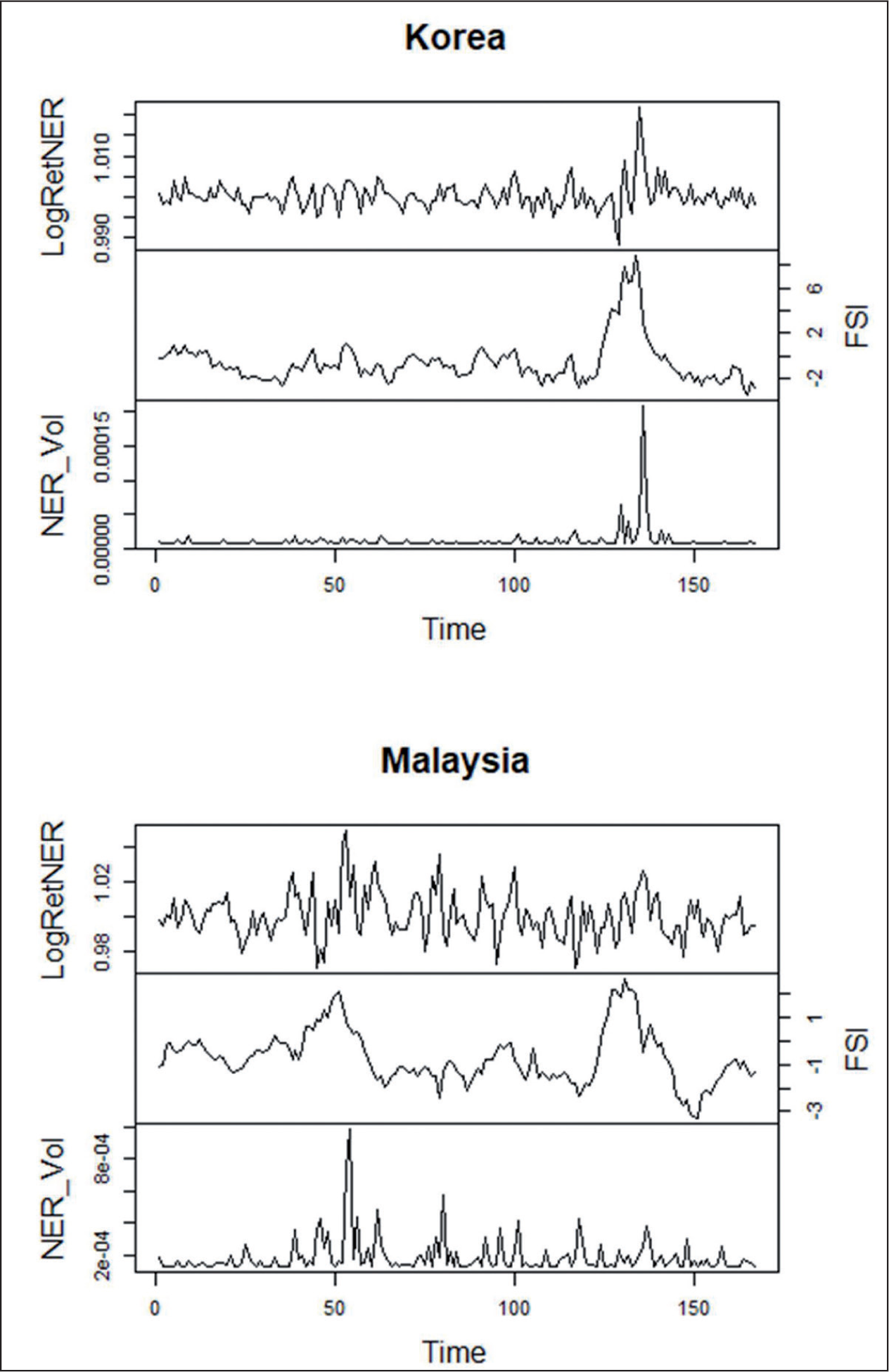
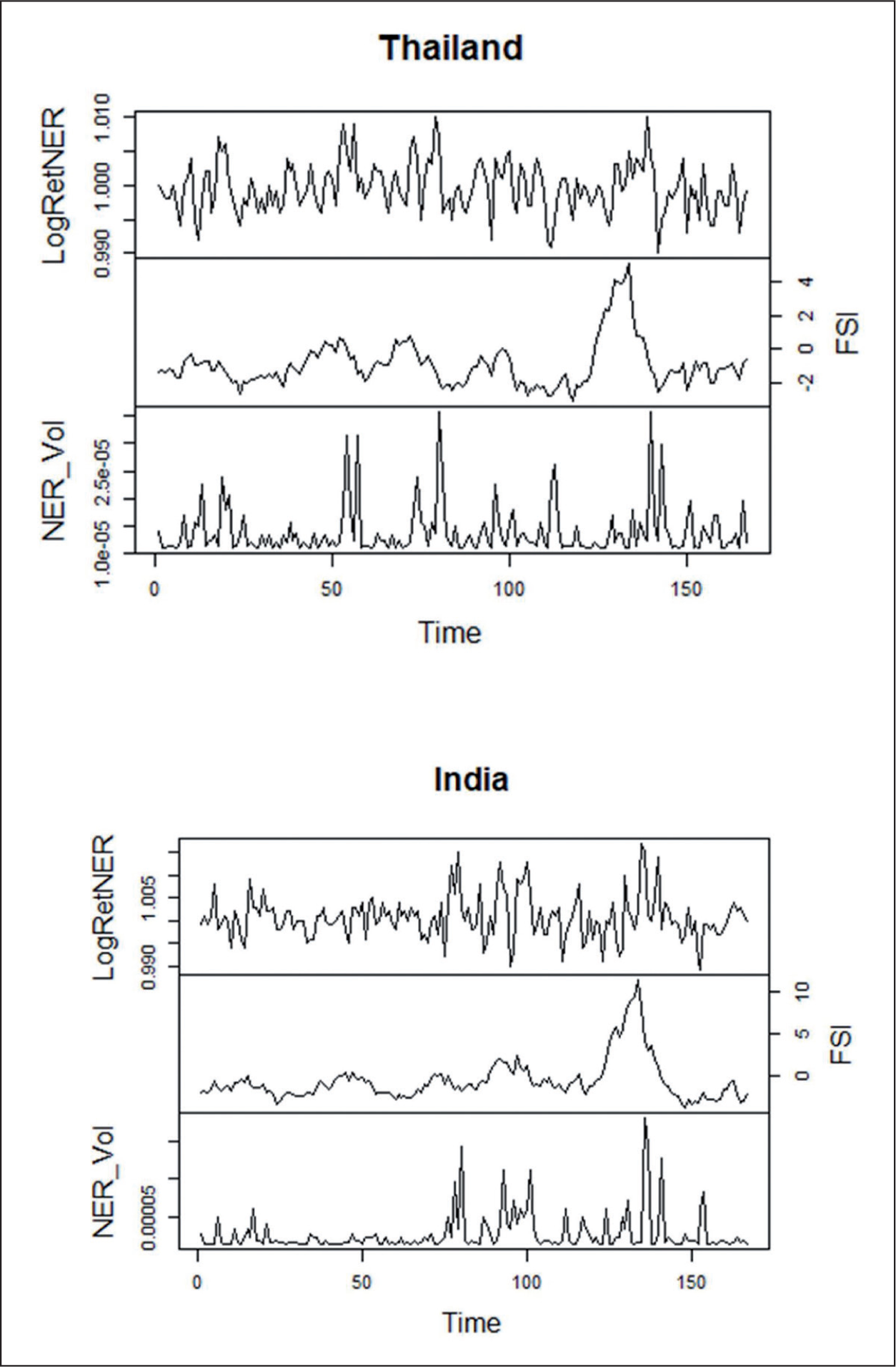
We have used widely adopted form of analysis of exchange rates using volatility of exchange rate return using monthly average nominal exchange rate (NER) of domestic currencies in terms of US dollars. The data are sourced from ADB for the period of 2006–2019. First, the volatility in log return of NER (R_NER is log return of NER) of the seven domestic currencies is calculated (see Figure 1). Second, using ADB’s country-specific Financial Stress Index (ADB_FSI), as a parsimonious measure of financial stress for the identified developing Asian nations, we examine the impact and persistence of the impact of financial stress on exchange rate volatility using vector autoregressive (VAR) model and impulse response function (IRF). Finally, we establish the predictive causality of exchange rate volatility with index of financial stress using the Granger causality tests. We conclude with implications of the study on financial fragilities, exchange rate regimes, policy coordination, monetary union, intra-regional trade, and FDI in developing Asia.

Figure 1.

Source: The authors (based on Economic and Financial Indicators Database of Asia Regional Integration Centre, Asian Development Bank).

2. Review of Literature: Exchange Rate Volatility and Financial Stress

2.1 Measuring Financial Stress

Preliminary studies by Kaminsky and Reinhart (1996, 1999) and Frankel and Rose (1996) indicated presence of exogenous factors inducing financial stress with the help of binary variables; a shock variable assumes the value of zero or one based on the presence or absence of financial crisis. But as observed by Illing and Liu (2006), the addition of binary variables to indicate presence or absence of crisis do not surmise the severity of the stress levels.

Existing literature establishes stress levels as a continuous measure of volatility in financial markets, including banking, foreign exchange, debt markets, and stock prices (Fischer, 2020; González-Hermosillo & Hesse, 2011). Stress transmission has been extended with the directional measure of within and across country cross-market volatility (Diebold & Yilmaz, 2012). Initially, Bordo et al. (2000) developed an index for the United States based on bank losses, business failures, real interest rates, and bond-yield spreads. Based on this methodology and combined with stock market indicators, BCA Research developed a monthly FSI for the United States. J. P. Morgan Chase & Co. developed a global liquidity, credit, and volatility index (LCVI) based on daily bond, foreign exchange, and stock market indicators (Kantor & Caglayan, 2002). Similarly, the FSI developed by Illing and Liu (2003), measures financial stress for Canada.

2.2 Financial Stress in Emerging Economies

Distinct in its approach, FSI developed for International Monetary Fund (IMF) by Danninger et al. (2009), proposed different measures of FSI for emerging economies and advanced economies due to “country-specific financial and trade linkages, structural characteristics, and vulnerabilities or policies, such as current account and budget imbalances.” Based on this, Park and Mercado (2014) developed an FSI (ADB_FSI) of ASEAN and developing Asian countries for ADB. The ADB_FSI is a composite index that measures the degree of financial stress in four financial markets—banks, foreign exchange, equity, and bonds. The country-specific FSI of member economies is derived from the composite index using variance equal weights and principal component analysis.

Existing literature establishes that exchange rate volatility does increase proportionally with the global financial stress (Coudert et al., 2011), but its predictive causality to detect periods of financial stress can be further explored. While investigating volatility spillovers, directional spillover and transmission of volatility has been observed from stock market to foreign exchange market; spillover “bursts” have been found more profound during crises periods (Diebold & Yilmaz, 2009). Furthermore, existing research provides empirical evidence of quantifying financial stress and its spillover distinctly for emerging economies (Moyo & Le Roux, 2020; Mundra & Bicchal, 2020). A robust model to understand the trend and interaction of exchange rate volatility and financial stress is an evident research gap in the context of developing nations. In the context of developing Asia, where financial markets are less mature and economic instability contributes to the extent of exogenous shocks, we aim to answer the research question, what is the impact of financial stress in inducing exchange rate volatility in developing Asia?

3. Methodology and Data

Exchange rates, like other financial time series data, exhibits wide swings over an extended time period; “followed by periods in which there is relative calm” (Gujarati & Porter, 2009). One of the fundamental methods adopted for modelling and predicting these swings or dispersion is attributed to Engle’s (1982) autoregressive conditional heteroscedascity (ARCH) or modelling the “varying variance” of financial time series. The presence of ARCH effect is confirmed by statistically significant error variance of the lagged terms of the series. Upon confirming the ARCH effect, Bollerslev’s (1986) generalized autoregressive conditional heteroscedascity (GARCH) has been adopted in the existing literature, wherein a GARCH (p, q) model suggests p lagged terms of the squared error with q terms of the lagged conditional variances. The simplest GARCH model is the ARCH (1) process a₁, a₂ … when $a_{t} = σ_{t} ε_{t} σ_{t}^{2} = ω + α_{1} a_{t - 1}^{2}$

But the ARCH (1) model does not have sufficient parameters to provide a good fit (Ruppert & Matteson, 2011). Mathematically, the representation of GARCH (1,0) denotes $σ_{t}^{2} = σ^{2} (1 - β) + 0 \times ε_{t - 1}^{2} + β σ_{t - 1}^{2},$ where $α_{0 i} > 0$ for some i when p > 0 (Francq & Zakoian, 2004).

Literature cites that in GARCH (1,0) model, the confidence intervals are time varying. This enables sub-periods of time with larger or smaller volatility (Ruppert & Matteson, 2011). The GARCH structure allows a more flexible lag structure as compared with ARCH specification (Cloquette et al., 1995). This is brought by a more intelligent model with smoother fitting of the conditional second moments, including their lagged term (Bollerslev, 1986). Zivot (2009) argues that low-order GARCH models are preferred over ARCH(p) models due to parsimony and numerical stability.

3.1 Modelling Exchange Rate Volatility: Data and Methods

To understand the trend and interaction of exchange rate volatility with financial stress, we use country-level monthly data from the period of 2006–2019 for seven representative economies of developing Asia, namely, Philippines, Indonesia, Malaysia, India, Republic of Korea, Singapore, and Thailand. The period of analysis is chosen to avoid the skewed impact of the 1997 Asian crisis on developing Asia, while reflecting the impact of global crisis of 2007–2008 (Haque & Varela, 2010). To ensure that the findings established through statistical techniques are valid and reliable, it is important to establish sample size adequacy. We have two major endogenous variables, namely, exchange rate volatility and FSI. The total number of observations required per cross-section is 2 × 10, that is, 20 (Hair et al., 1995). But a larger sample size will ensure efficient estimate of the coefficients. In our sample, we have 156 data points of each country, hence, the sample is adequate to accurately run financial time series analysis.

From country-level monthly data of NER, we construct log returns of NER, that is, R_NER. Here, R_NER = $\ln (\frac{N E R_{t + 1}}{N E R_{t}}) = \ln (1 + r)$ .

Further, volatility clustering is observed by graphically plotting R_NER as a time series. Thereafter, we have used the simplest form of volatility model GARCH (1,0), which can be written as: $σ_{t}^{2} (R_{N E R}) = α_{0} + α_{1} u_{t - 1}^{2} + α_{2} σ_{t - 1}^{2} (R_{N E R})$ ; (where $σ_{t}^{2} (R_{N E R})$ is volatility of the NER return) here conditional variance u at time t depends on squared error term is the previous period $(α_{1} u_{t - 1}^{2})$ , that is, the ARCH (1) model, and also on the conditional variance in the previous time period $α_{2} σ_{t - 1}^{2} (R_{N E R})$ . We chose GARCH (1,0) model here based on the Akaike information criterion (AIC) and the Hannan–Quinn information criterion (HQIC). Based on the minimum information theoretical criterion estimate, AIC assigns a penalty factor of two for the number of independently adjusted parameters in the model. Thus, AIC = 2k – p ln(L), where k is number of parameters in the model, p is penalty factor, and ln(L) is the log likelihood estimates of the parameters. As per classical likelihood estimation procedure of statistical model identification, the maximum log likelihood estimate of the model parameters is obtained for the minimum value of AIC (Akaike, 1974; Lee & Phillips, 2015). Our model adequacy significantly improves with the minimum value of AIC reported for GARCH (1,0) model. Given our large sample size, we recheck the model adequacy with reference to HQIC. GARCH (1,0) reports the least value of HQIC, confirming that the best approximate of the lagged term is of the order p = 1 defining the volatility model (Shono, 2005).

Though there exists theoretical and empirical evidence of AIC being the best estimator of GARCH (p, q) models for p, q ≤ 2 (Zivot, 2009), we have derived the auto-correlation function (ACF) and partial auto-correlation function (PACF) of the conditional variance obtained from the GARCH (1,0) model to infer model sufficiency; the values are close to zero, which ascertains the model adequacy¹ (Ruppert & Matteson, 2011; Yussof et al., 2016).

While determining model fitness of GARCH (1,0), Engle and Ng’s (1993) test statistics² reveal that there is no evidence of positive or negative bias. Hence, the model is able to capture asymmetric volatility with no bias effect of either positive or negative shocks (Lundbergh & Terasvirta, 2002).

From the GARCH (1,0) model, we construct a numeric vector NER_Vol with the conditional variances, that is, the unconditional variance combined with the deviation of squared error from its average value for each domestic currency. Here, NER_Vol can be denoted as $σ_{t - 1}^{2} (R_{N E R})$ , that is, conditional variance of the GARCH (1,0) model that uses the historic values to forecast the variance, to measure volatility. Statistically, the volatility clustering in NER_Vol will imply higher levels of dispersion in NER returns over a period of time.

To study the trend of financial stress, we consider country specific ADB_FSI as a parsimonious measure (Park & Mercado, 2013). It is denoted as:

ADB_FSI = β + Stockreturns + Stockvolatility + Debtspreads + EMPI, where

β = $\frac{cov (r, m)}{var (m)}$ , where r is the returns of the banking sector stock price index and m is the overall stock price index;

Stockreturns ≥ ln(γ_t)−ln(γ_t₋₁), γ_t is equity return;

Stockvolatility follows GARCH (1,1) process for γ_t = α_i,t + βγ_t−1 + ε_i,t given by σ²t = ω + φ₁ ε²t₋₁ + φ₂ σ²t₋₁.

Debtspreads is the yield differentials between long-term (10-year) local government bonds and short-term (2-year) local government bonds;

EMPI_i,t = $\frac{(Δ e_{i, t} - μ_{i, Δ e})}{σ_{i^{, Δ e}}} - \frac{Δ R E S_{i, t} - μ_{i, Δ R E S}}{σ_{i, Δ R E S}}$ , where Δe and ΔRES are month-on-month percent changes in the foreign exchange rate of US dollar-denominated local currency and foreign exchange reserves, respectively.

The country-level monthly ADB_FSI index is plotted against the corresponding R_NER.

R_NER, FSI and NER_Vol are reported stationary using augmented Dickey–Fuller (ADF) test (see Table 2).

Table 2.
Augmented Dickey–Fuller (ADF) test and Kwiatkowski–Phillips–Schmidt–Shin (KPSS) test

p-Value India
Indonesia
Korea
Malaysia
Philippines
Singapore
Thailand

ADF KPSS ADF KPSS ADF KPSS ADF KPSS ADF KPSS ADF KPSS ADF KPSS

LogReturnNER¹ 0.01*** 0.1* 0.01*** 0.1* 0.01*** 0.1* 0.01*** 0.1* 0.01*** 0.1* 0.01*** 0.09* 0.01*** 0.1*

FSI² 0.01* 0.05 0.05** 0.1* 0.01*** 0.1* 0.08* 0.1* 0.03** 0.1* 0.03** 0.09* 0.01*** 0.1*

NER volatility 0.01* 0.04 0.01*** 0.1* 0.04*** 0.09* 0.01*** 0.1* 0.01* 0.01* 0.01*** 0.1* 0.01*** 0.1*

p-Value	India	Indonesia	Korea	Malaysia	Philippines	Singapore	Thailand
LogReturnNER¹	0.01***	0.1*	0.01***	0.1*	0.01***	0.1*	0.01***	0.1*	0.01***	0.1*	0.01***	0.09*	0.01***	0.1*
FSI²	0.01***	0.05**	0.05**	0.1*	0.01***	0.1*	0.08*	0.1*	0.03**	0.1*	0.03**	0.09*	0.01***	0.1*
NER volatility	0.01***	0.04**	0.01***	0.1*	0.04***	0.09*	0.01***	0.1*	0.01***	0.01***	0.01***	0.1*	0.01***	0.1*

Source: The authors (based on Economic and Financial Indicators Database of Asia Regional Integration Centre, Asian Development Bank).

Notes: ***, **, and * denote significance at the 1%, 5%, and 10% levels, respectively.

¹ KPSS test for trend stationarity.

² The model for FSI includes a trend for India, P.R. Korea, and Singapore.

In addition to ADF test, we performed Kwiatkowski–Phillips–Schmidt–Shin (KPSS) test on FSI, RNER, and NER_Vol. Otero and Smith (2005) suggest that the KPSS test statistics compliment the inference of ADF with indication of permanent changes in the intercept, that is, the trend in the time series. KPSS test reports that FSI is trend stationary, whereas RNER and NER_Vol is level stationary with lag parameter of four. The trend stationarity present in FSI implies that even though there are episodes of shock (volatility clustering), the series retracts to its original path which is established by the model KPSS equation for a significant period of four quarters.

We further analyze the interaction and relationship of NER return volatility and ADB_FSI using the VAR and Granger causality to test the hypothesis that there exists predictive causality between FSI and foreign exchange rate volatility. As ADB_FSI includes exchange market pressure index based on standardized return and standardized foreign exchange reserve, we have done the VAR and Granger causality estimation using volatility of exchange rate rather than exchange rate return or foreign exchange reserve.

4. Results and Discussion

4.1 Volatility Clustering

We analyzed the trend of R_NER by plotting it as a time series to graphically detect volatility clustering (see Figure 1). Volatility clustering was also confirmed by ARCH test.

Period of higher volatility was observed for India, Philippines, Malaysia, and Thailand; whereas Korea and Singapore had lower volatility spikes. A lesser dispersion is a reflection of the Singapore’s effective exchange rate management as a dynamic small open economy; the highest single surge in the third month of 2011 reflects the instability caused due to the year’s general election (Tan, 2012). As for Korea, lower volatility is a result of the Bank of Korea’s “smoothing operations” to minimize swings in exchange rate (Rajan, 2012). Indonesia recorded the least volatility clustering, with market demand and supply wholly determining the exchange rate of the rupiah. Further, though Indonesia’s monetary policy resembles the inflation targeting framework of most of the emerging market economies, the base money operational target was replaced in 2005 with policy rate as a reference in monetary control (Tan, 2012).

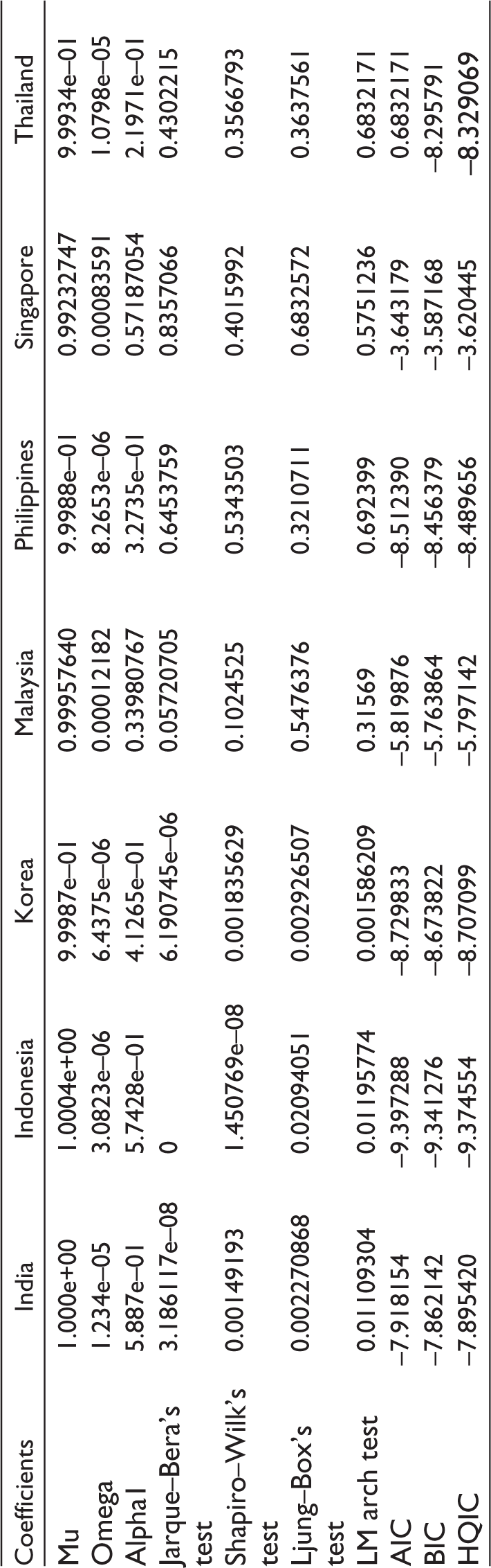
Using the AIC and HQIC, R_NER is modeled using GARCH (1,0) method for India, Indonesia, Malaysia, Singapore, Philippines, Thailand, and Republic of Korea. Further, the model confirmed the normality and auto-correlation of the standardized residuals of respective country series of R_NER through Jarque–Bera test and Ljung–Box test, respectively (Bera & Jarque, 1981). This conforms to the existing empirical studies of exchange rate wherein GARCH (1,0) is employed for volatility modelling (Koutmos & Martin, 2003; Ramachandran & Srinivasan, 2007). The results of the model are presented in Table 3.

Table 3.
Coefficients and Standardized Residual Tests of GARCH (1,0)—LogReturnNER

Coefficients India Indonesia Korea Malaysia Philippines Singapore Thailand

Mu 1.000e+00 1.0004e+00 9.9987e–01 0.99957640 9.9988e–01 0.99232747 9.9934e–01

Omega 1.234e–05 3.0823e–06 6.4375e–06 0.00012182 8.2653e–06 0.00083591 1.0798e–05

Alpha1 5.887e–01 5.7428e–01 4.1265e–01 0.33980767 3.2735e–01 0.57187054 2.1971e–01

Jarque–Bera’s test 3.186117e–08 0 6.190745e–06 0.05720705 0.6453759 0.8357066 0.4302215

Shapiro–Wilk’s test 0.00149193 1.450769e–08 0.001835629 0.1024525 0.5343503 0.4015992 0.3566793

Ljung–Box’s test 0.002270868 0.02094051 0.002926507 0.5476376 0.3210711 0.6832572 0.3637561

LM arch test 0.01109304 0.01195774 0.001586209 0.31569 0.692399 0.5751236 0.6832171

AIC –7.918154 –9.397288 –8.729833 –5.819876 –8.512390 –3.643179 0.6832171

BIC –7.862142 –9.341276 –8.673822 –5.763864 –8.456379 –3.587168 –8.295791

HQIC –7.895420 –9.374554 –8.707099 –5.797142 –8.489656 –3.620445 –8.329069

Coefficients	India	Indonesia	Korea	Malaysia	Philippines	Singapore	Thailand
Mu	1.000e+00	1.0004e+00	9.9987e–01	0.99957640	9.9988e–01	0.99232747	9.9934e–01
Omega	1.234e–05	3.0823e–06	6.4375e–06	0.00012182	8.2653e–06	0.00083591	1.0798e–05
Alpha1	5.887e–01	5.7428e–01	4.1265e–01	0.33980767	3.2735e–01	0.57187054	2.1971e–01
Jarque–Bera’s test	3.186117e–08	0	6.190745e–06	0.05720705	0.6453759	0.8357066	0.4302215
Shapiro–Wilk’s test	0.00149193	1.450769e–08	0.001835629	0.1024525	0.5343503	0.4015992	0.3566793
Ljung–Box’s test	0.002270868	0.02094051	0.002926507	0.5476376	0.3210711	0.6832572	0.3637561
LM arch test	0.01109304	0.01195774	0.001586209	0.31569	0.692399	0.5751236	0.6832171
AIC	–7.918154	–9.397288	–8.729833	–5.819876	–8.512390	–3.643179	0.6832171
BIC	–7.862142	–9.341276	–8.673822	–5.763864	–8.456379	–3.587168	–8.295791
HQIC	–7.895420	–9.374554	–8.707099	–5.797142	–8.489656	–3.620445	–8.329069

Source: The authors (based on Economic and Financial Indicators Database of Asia Regional Integration Centre, Asian Development Bank).

We use conditional variance of GARCH (1,0) to construct the numeric vector NER_Vol. Plotted to understand the error variances, the volatility clustering in NER_Vol implies higher levels of dispersion in NER returns over a period of time (see Figure 1).

4.2 Interaction of Financial Stress and Exchange Rate Volatility

Upon finding NER_Vol and country-specific ADB_FSI as stationary, we identify VAR model from existing literature to test bilateral causality for multiple timeseries variables in a single model. At its core, the VAR model is an extension of the univariate autoregressive model or AR(p) model where a vector of time series variables is regressed on lagged vectors of these variables. Hence, our VAR (pp) model of two variables ADB_FSI & NER_Vol is given by:

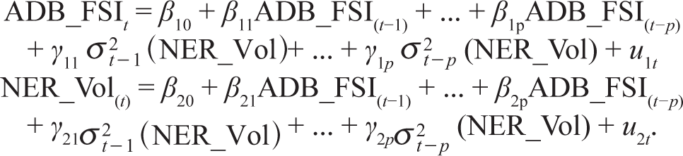
\begin{array}{l} A D B_F S I_{t} = β_{10} + β_{11} A D B_F S I_{(t - 1)} + \dots + β_{1 p} A D B_F S I_{(t - p)} \\ + γ_{11} σ_{t - 1}^{2} (N E R_V o l) + \dots + γ_{1 p} σ_{t - p}^{2} (N E R_V o l) + u_{1 t} \\ N E R_V o l_{(t)} = β_{20} + β_{21} A D B_F S I_{(t - 1)} + \dots + β_{2 p} A D B_F S I_{(t - p)} \\ + γ 21 σ_{t - 1}^{2} (N E R_V o l) + \dots + γ_{2 p} σ_{t - p}^{2} (N E R_V o l) + u_{2 t} . \end{array}

β and γ are estimated using VAR approach.³ We arrive on the lag length of VAR of p = 1 using information criteria of the models. For a multiple equation model, we choose the specification which has the smallest BIC (p), where BIC (p) = log[det( ${\hat{Σ}}_{u}$ )] + k(kp+1) $\frac{\log (T)}{T}$ , where ${\hat{Σ}}_{u}$ denotes the estimate of the k × k covariance matrix of the VAR errors and det (.) denotes the determinant.

The covariance matrix of VAR residuals can be further expressed as $cov (u_{i}) = (y_{i} - \hat{y_{i}})$ ; hence, the smaller the variance of residuals, the closer is the value of $\hat{y_{i}}$ to $y_{i}$ . Covariance of residuals was closer to zero for all, which implies that the fit of the model was proper.⁴ We report $cov (e_{F S I}, e_{N E R_{V O L}})$ as –4.670e–06 for India, –1.985e–06 for Indonesia, –2.967e–06 for Korea, 3.118e–06 for Malaysia, –2.669e-07 for Philippines, –3.830e-04 for Singapore, and –3.466e-07 for Thailand (see Table 4). Here, we establish the interaction between NER_Vol & ADB_FSI through VAR (1) that there exists predictive causal relationship between FSI and foreign exchange rate volatility.

Table 4.
Covariance and Correlation Matrix of Residuals of VAR Model: FSI and Volatility (NER_Vol)

COV_{FSI, volatility} India Indonesia Korea Malaysia Philippines Singapore Thailand

–4.670e–06 –1.985e–06 –2.967e–06 3.118e–06 –2.669e–07 –3.830e–04 –3.466e–07

C_{FSI, volatility} –0.2412 –0.486 –0.298 0.08627 –0.09661 –0.2594 –0.1434

COV_{FSI, volatility}	India	Indonesia	Korea	Malaysia	Philippines	Singapore	Thailand
–4.670e–06	–1.985e–06	–2.967e–06	3.118e–06	–2.669e–07	–3.830e–04	–3.466e–07
C_{FSI, volatility}	–0.2412	–0.486	–0.298	0.08627	–0.09661	–0.2594	–0.1434

Source: The authors (based on Economic and Financial Indicators Database of Asia Regional Integration Centre, Asian Development Bank).

The correlation matrix of VAR residuals reflects negative correlation between financial stress and exchange rate volatility in India, Indonesia, Korea, Singapore, and Thailand, with weakest negative correlation for Philippines (see Table 4). This corroborates that reduction in economic activity induces higher levels of exchange rate volatility. Weak positive correlation is reported for VAR residuals of Malaysia, reflecting the Malaysian Central Bank’s passive interventions to minimize volatility and fundamental misalignments.

4.3 Impact of Financial Stress on Exchange Rate Volatility

To further explain the impact of financial stress on exchange rate volatility, we plot the orthogonal IRF from country-specific ADB_FSI on respective NER_Vol of domestic currencies (see Figure 2). IRF establishes their interaction without establishing the endogeneity or exogeneity of either of the variables.

Figure 2.

Source: The authors (based on Economic and Financial Indicators Database of Asia Regional Integration Centre, Asian Development Bank).

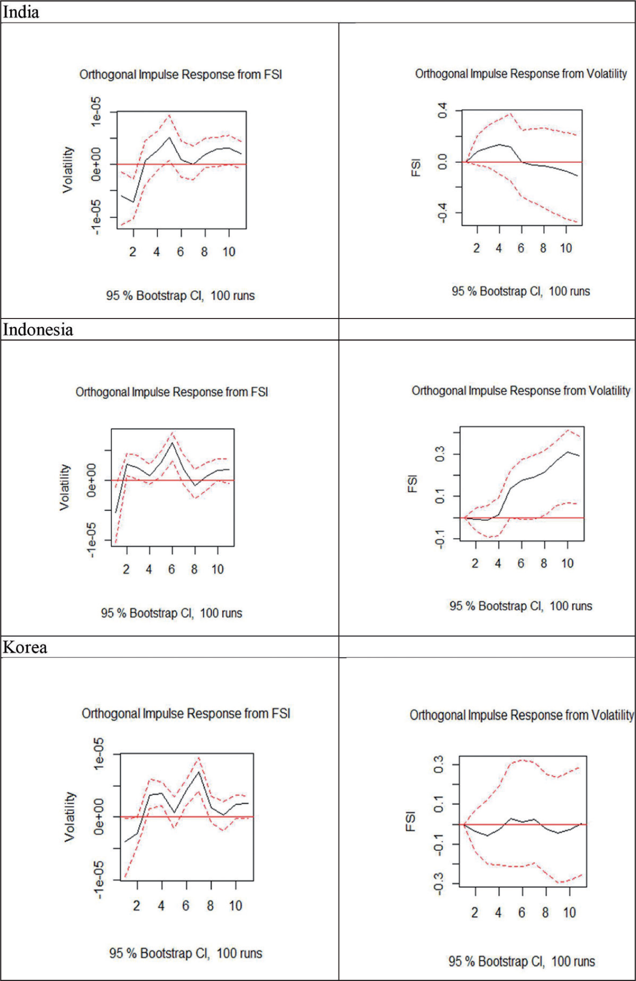
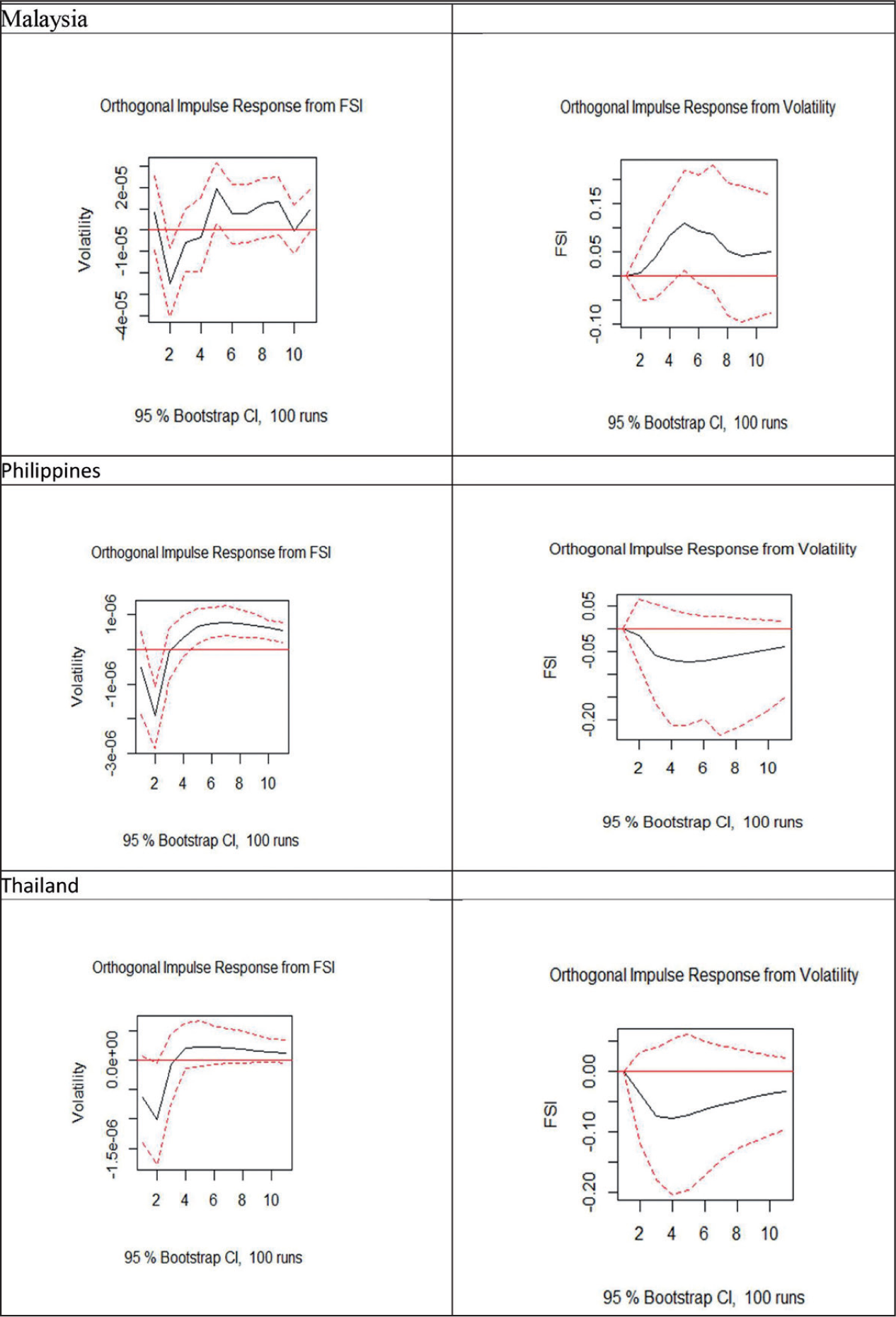
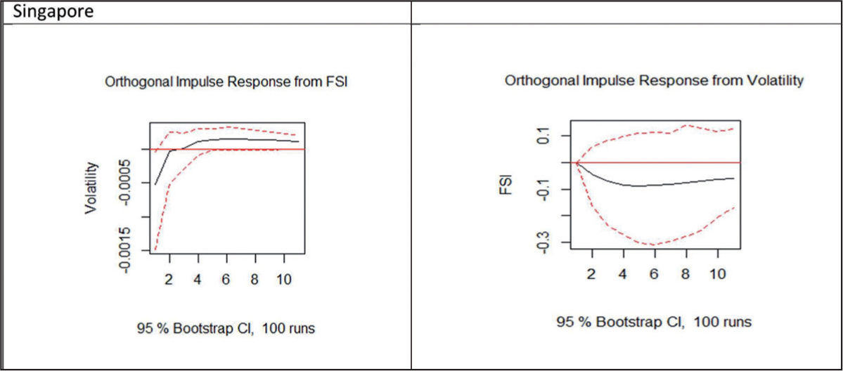
For most of the countries, we have analyzed that there was a decrease in volatility in exchange rate returns till 2 months after a shock in the FSI after which the volatility increased. The reduction in volatility in exchange rate can be explained through sudden stop phenomenon⁵. In particular, it can be attributed to a sudden decline in capital flow and resultant economic activity in the economy (Eichengreen & Gupta, 2016). However, the peak of volatility in exchange differs from country to country. Except for India and Indonesia, the impact of ADB_FSI on volatility was found to last longer. Careful interventions of the central banks to prevent excessive fluctuations in domestic currency may have led to the shorter response for India and Indonesia. The positive impact of FSI on exchange rate volatility was observed for eight months in the case of Korea, Malaysia, Philippines, Thailand, and Singapore, with the peak in volatility observed around the 6th month. Philippines, Thailand, and Malaysia reported the strongest impact of FSI on NER return volatility.

However, except for Indonesia, exchange rate volatility did not intrinsically lead to higher levels of financial stress (see Figure 2).

In the case of Indonesia, the impulse response from exchange rate volatility to FSI was seen to have substantial deviation from zero. In previous studies, different reactions of exchange rate to financial stress were observed in the Euro area (Elbourne et al., 2018). In the case of Indonesia, diversification of export and focus on manufacturing attracted FDI which could be one of the reasons why different reactions can be observed in terms of the impact of exchange rate volatility on financial stress. World Bank’s economic outlook of 2018 stated that “expanding exports, reducing fuel imports, and boosting FDI, especially in export-oriented industries” have strengthened Indonesian economy in contrast to the period of high deficits in the fixed exchange rate regime before 1997 (Chaves, 2018).

4.4 Predictive Causality of Financial Stress and Exchange Rate Volatility

When applied on NER_Vol & ADB_FSI, Granger’s causality reports significant F statistics, that is, predictive causality bi-directionally for India, Korea, Philippines, and Thailand (see Table 5). Indonesia reports a significant predictive causality of NER_Vol on the FSI levels, whereas, Malaysia and Singapore report significant predictive causality of FSI on NER returns.

Table 5.
Granger’s Causality—p-Value of F Statistic

H0: FSI do not Granger-cause volatility

India Indonesia Korea Malaysia Philippines Singapore Thailand

F statistics 4.2337 14.056 11.951 3.1709 17.224 1.8274 4.2592

p-Value 0.0009805* 2.2e–16* 2.163e–13* 0.001851* 7.863e–08* 0.1625 0.01494*

H0: Volatility do not Granger-cause FSI

India Indonesia Korea Malaysia Philippines Singapore Thailand

F statistics 1.4188 3.1226 0.46708 0.74626 0.7555 0.38468 0.76087

p-Value 0.2172 0.001344*** 0.858 0.6506 0.4706 0.681 0.4681

H0: FSI do not Granger-cause volatility
F statistics	4.2337	14.056	11.951	3.1709	17.224	1.8274	4.2592
p-Value	0.0009805***	2.2e–16***	2.163e–13***	0.001851***	7.863e–08***	0.1625	0.01494***
H0: Volatility do not Granger-cause FSI
	India	Indonesia	Korea	Malaysia	Philippines	Singapore	Thailand
F statistics	1.4188	3.1226	0.46708	0.74626	0.7555	0.38468	0.76087
p-Value	0.2172	0.001344***	0.858	0.6506	0.4706	0.681	0.4681

Source: The authors (based on Economic and Financial Indicators Database of Asia Regional Integration Centre, Asian Development Bank).

Note: *** denotes significance at 1% level.

This corroborates with empirical evidence that exchange rate volatility increased with global financial stress, but it contradicts that the stress has to be pervasive globally or the increase in NER volatility is proportionate with the financial stress (Coudert et al., 2011). Our results correspond to the non-linear impact of exchange rate volatility on financial stress experienced in Central and Eastern Europe (CEE), with an exception that for developing Asia, we find evidence of bi-directional causality (Adam et al, 2018).

We extend this predictive causality with the findings from the IRFs and Granger’s causality tests to suggest that in developing Asia, the impact of financial stress is significant in inducing foreign exchange rate volatility. Existing research suggests that stress is driven by multiple factors and management of exchange rate volatility in emerging economies will need to address problems not only in the foreign exchange market but also in the other financial sectors, including banking sector, equity, and bond markets (Balakrishnan et al., 2011).

5. Implications and Conclusion

With evidence of volatility clustering in NER of dollar-denominated domestic currencies of developing Asia, we contribute to the existing literature of exchange rate volatility of emerging economies where instability in financial markets contributes to the extent of exogenous shocks. In the following subsections, we discuss implications of our findings with deeper insights on interaction of exchange rate volatility and financial stress in developing Asia.

5.1 Implications of Financial Fragilities

This study provides empirical evidence that the predictive causal relationship of financial stress and exchange rate volatility is negatively correlated, except for Malaysia where the central bank’s interventions to refute misalignments reflect a positive correlation. This further corroborates with the impulse response from financial stress impacting volatility of dollar-denominated exchange rates up to 8 months. The role of financial stress in inducing exchange rate volatility in the context of emerging markets, especially developing Asian nations, is monotonic. A spike in stress may lead to reduced economic activity, decreased confidence in the economy and capital flight (Doner, 2018). Within a period of heightened stress, developing Asian nations may experience cross market volatility spillovers from foreign exchange rate to stock, bond and commodities market (Diebold & Yilmaz, 2012). We, hence, provide empirical evidence that volatility in foreign exchange rate is magnified by the financial fragilities of an economy. This provides a future scope of research to investigate the transmission and directional spillover of cross market volatility in developing Asia.

Corroborating with the third-generation model of currency crises, which treats depreciation of NERs as a symptom and cites foreign currency-denominated debts and flight of capital as fundamental causes, our study implicates the strength of the financial system in developing Asian nations that impacts the level and spread of stress, inducing exchange rate volatility.

5.2 Volatility and Implications of Foreign Direct Investment

An important policy implication is the diverse structure of FDI in the developing Asian region. Here, it is important to note that though depreciation of the local currency of the host country may attract FDI, high volatility in the local exchange rate discourages in-bound FDI (Kiyota & Urata, 2004; Latief & Lefen, 2018). To mitigate stress at regional level, it is penultimate to make the business environment conducive to attract FDI. This has further empirical evidence, wherein FDI being strategically directed in locations across India, Indonesia, Malaysia, Philippines, and Thailand to circumvent the volatility of local exchange rates (Gottschalk & Hall, 2008).

5.3 Exchange Rate Regimes and Volatility

While we examine volatility clustering, it is evident that India, Philippines, Malaysia, and Thailand have more frequent periods of NER volatility as compared with Singapore, Indonesia, and Korea. We further corroborate the observed volatility with exchange rate regimes. Singapore dollar follows managed float (International Monetary Fund [IMF], 2019), but has experienced lesser episodes of volatility as the basket of currencies is trade-weighted and the policy band is allowed to fluctuate. In case of Indonesia and Korea, exchange rates are determined by demand and supply of currency, though there are smoothing operations by respective central banks to avoid excessive fluctuations (Rajan, 2012). This corresponds to empirical evidence that higher flexibility in exchange rate regimes lead to lesser volatility (Combes at al., 2012).

In developing Asia, countries who have officially adopted floating exchange rates exhibit “fear of floating” by intervening passively (Rizvi et al., 2017). The strategy of Asian nations to stabilize exchange rate volatility against the US dollar is suboptimal owing to its informal and uncoordinated approach (Kawai, 2002). But considering that developing Asian nations opt for inflation-targeting regimes, implementing optimized interest rates remain an observed commonality within the region. Hence, there is a scope for policy-coordinated inflation targeting within developing Asia to address exchange rate volatility; this may further lead to reduction in financial stress levels (Alexandre et al., 2002; Park & Son, 2021; Woodford, 2012).

5.4 Policy Coordination and Monetary Union

Focusing on policy coordination, harmonizing their fiscal policy as inflation targeting economies is long-term goal and difficult to achieve, given the geopolitical dynamics of developing Asia. However, independently they can move towards monetary union. Extensive intra-regional trade of East and South East Asia gives an opportunity for a common basket of currencies which may stabilize intra-regional exchange rates and reduce financial stress by promoting trade, investment, and growth in the region. Suggestions of a basket of tripolar currency has been made in the past, consisting of the US dollar, the Japanese Yen, and the Euro. During incidences of heightened financial stress leading towards pertinent crisis, formal pegs (currency board, crawling, or basket with margins) need to be suspended. Developing Asian nations need to maintain their own formal exchange rate mechanism and a regional exchange rate arrangement which focuses on intraregional stability and regional economic growth (Kawai, 2002; Shimizu & Sato 2018).

5.5 Implications of Intra-regional Trade

A step forward to intraregional economic growth for developing Asia is regional cooperation in international trade. While seminal literature establishes both negative and positive relationship of exchange rate volatility and international trade (McKenzie, 1999), their negative relationship, more impactful than tariffs, has been empirically observed for developing Asia, especially East Asia, which extensively relies on intra-regional trade (Hayakawa & Kimura, 2009).

Trade cooperation through charters of Association of Southeast Asian Nations (ASEAN), Asia-Pacific Economic Cooperation (APEC), and most recently by Regional Comprehensive Economic Partnership (RCEP) has achieved renewed focus. But intra-regional trade in Asia, especially East Asia, is predominated by production networks and the ramifications of exchange rate volatility are different. The production networks contribute to more than 50% of manufacturing trade exports in developing Asia, with Philippines at 87.3%; Korea at 69.5%; Malaysia at 78.8%; Singapore at 66.5%; Thailand at 62.9%; and Indonesia at 38.4% of its manufacturing exports (Athukorala, 2011). But these networks are intricate and typically dependent on long-standing relationships of business partners which are built over a period of time. An increase in exchange rate volatility reduces exports of intermediate goods from Asia. This further reduces the intra-regional trade flow, reducing economic activity in the region and increasing financial stress (Okubo et al., 2014; Thorbecke, 2008).

We therefore underline the implications of de-facto pegging in developing Asia, with covert interventions of respective central banks leading to higher exchange rate volatility. Our results highlight the need for developing different sub-markets of the financial sector, macroeconomic policy coordination through harmonizing fiscal policy and a focus towards monetary union. These measures are expected to reduce exchange rate volatility and mitigate financial stress thereby supporting intra-regional trade and production network. With empirical evidence of differential impact on differentiated goods and trade channels, policy measures need to capture the idiosyncrasies of each industry, sector and sub-sector of a country, taking into account the dynamics of exchange rate volatility, and financial stress.

Footnotes

Declaration of Conflicting Interests

The authors declared no potential conflicts of interest with respect to the research, authorship, and/or publication of this article.

Funding

The authors received no financial support for the research, authorship, and/or publication of this article.

Notes

References

Adam

, Benecká

, & Matějů

(2018). Financial stress and its non-linear impact on CEE exchange rates. Journal of Financial Stability, 36, 346–360.

Akaike

, (1974). A new look at the statistical model identification. IEEE Transactions on Automatic Control, 19(6), 716–723.

Alexandre

, Driffill

, & Spagnolo

(2002). Inflation targeting, exchange rate volatility and international policy coordination. The Manchester School, 70(4), 546–569.

Asian Development Bank (ADB). (2019). Operations manual policies and procedures (Section A1)—Classification and graduation of developing member countries (pp. 1–4). https://www.adb.org/sites/default/files/institutional-document/31483/om-a1.pdf

Athukorala

P. C.

(2011). Production networks and trade patterns in East Asia: Regionalization or globalization? Asian Economic Papers, 10(1), 65–95.

Balakrishnan

, Danninger

, Elekdag

, & Tytell

(2011). The transmission of financial stress from advanced to emerging economies. Emerging Markets Finance and Trade, 47(2), 40–68. 10.2753/REE1540-496X4703S203

Bera

A. K.

, & Jarque

C. M.

(1981). Efficient tests for normality, homoscedasticity and serial independence of regression residuals. Monte Carlo Evidence. Economics Letters, 7(4), 313–318. 10.1016/0165-1765(81)90035-5

Bernanke

, & Gertler

(2000). Monetary policy and asset price volatility (NBER Working Paper No. 7559). National Bureau of Economic Research.

Bjørnland

H. C.

(2009). Monetary policy and exchange rate overshooting: Dornbusch was right after all. Journal of International Economics, 79(1), 64–77.

10.

Bodart

, Candelon

, & Carpantier

J. F.

(2012). Real exchange rates in commodity producing countries: A reappraisal. Journal of International Money and Finance, 31(6), 1482–1502.

11.

Bollerslev

(1986). Generalized autoregressive conditional heteroskedasticity. Journal of Econometrics, 31(3), 307–327.

12.

Bordo

, Dueker

, & Wheelock

(2000). Aggregate price shocks and financial instability: An historical analysis (NBER Working Paper No. 7652). National Bureau of Economic Research.

13.

Chaves

(2018). Global financial markets and the Rupiah exchange rate. World Bank. https://www.worldbank.org/en/news/opinion/2018/10/03/global-financial-markets-and-the-rupiah-exchange-rate

14.

Cheung

Y. W.

, & Sengupta

(2013). Impact of exchange rate movements on exports: An analysis of Indian non-financial sector firms. Journal of International Money and Finance, 39, 231–245.

15.

Cloquette

J. F.

, Gérard

, & Hadhri

(1995). An empirical analysis of Belgian daily returns using GARCH models. Cahiers Économiques de Bruxelles, 418, 513–535.

16.

Combes

J. L.

, Kinda

, & Plane

(2012). Capital flows, exchange rate flexibility, and the real exchange rate. Journal of Macroeconomics, 34(4), 1034–1043.

17.

Coudert

, Couharde

, & Mignon

(2011). Exchange rate volatility across financial crises. Journal of Banking & Finance, 35(11), 3010–3018.

18.

Danninger

, Tytell

, Balakrishnan

, & Elekdag

(2009). The transmission of financial stress from advanced to emerging economies (IMF Working Paper No.133, 1–52). International Monetary Fund.

19.

Diebold

F. X.

, & Yilmaz

(2009). Measuring financial asset return and volatility spillovers, with application to global equity markets. The Economic Journal, 119(534), 158–171.

20.

Diebold

F. X.

, & Yilmaz

(2012). Better to give than to receive: Predictive directional measurement of volatility spillovers. International Journal of Forecasting, 28(1), 57–66. 10.1016/j.ijforecast.2011.02.006

21.

Doner

(2018). Politics and the growth of local capital in Southeast Asia: Auto industries in the Philippines and Thailand. In McVey

(Ed.), Southeast Asian capitalists (pp. 191–218). Cornell University Press.

22.

Eichengreen

, & Gupta

(2016). Managing sudden stops. World Bank. 10.1596/1813-9450-7639

23.

Elbourne

, Ji

, & Duijndam

(2018, February). The effects of unconventional monetary policy in the euro area. Proceeding of EUROFRAME conference. https://www.cpb.nl/sites/default/files/omnidownload/cpb-discussion-paper-371-the-effects-of-unconventional-monetary-policy-in-the-euro-area.pdf

24.

Engle

(1982). Autoregressive conditional heteroscedasticity with estimates of the variance of United Kingdom inflation. Econometrica: Journal of the Econometric Society, 50, 987–1007.

25.

Engle

R. F.

, & Ng

V. K.

(1993). Measuring and testing the impact of news on volatility. The Journal of finance, 48(5), 1749–1778.

26.

Fama

E. F.

, & French

K. R.

(2004). The capital asset pricing model: Theory and evidence. Journal of Economic Perspectives, 18(3), 25–46.

27.

Fischer

(2020). Monetary surprises and global financial flows: A case study of Latin America. Journal of Emerging Market Finance, 19(2), 189–225.

28.

Francq

, & Zakoian

J. M.

(2004). Maximum likelihood estimation of pure GARCH and ARMA-GARCH processes. Bernoulli, 10(4), 605–637.

29.

Frankel

, & Rose

(1996). Currency crashes in emerging markets: An empirical treatment. Journal of International Economics, 41, 351–366.

30.

González-Hermosillo

, & Hesse

(2011). Global market conditions and systemic risk. Journal of Emerging Market Finance, 10(2), 227–252.

31.

Gottschalk

, & Hall

(2008). Foreign direct investment and exchange rate uncertainty in South-East Asia. International Journal of Finance & Economics, 13(4), 349–359.

32.

Hair

J. F.

, Anderson

R. E.

, Tatham

R. L.

, & Black

W. C.

(1995). Multivariate data analysis. Prentice-Hall.

33.

Haque

, & Varela

(2010). US-Thailand bilateral safety-first portfolio optimisation around the 1997 Asian financial crisis. Journal of Emerging Market Finance, 9(2), 171–197.

34.

Hayakawa

, & Kimura

(2009). The effect of exchange rate volatility on international trade in East Asia. Journal of the Japanese and International Economies, 23(4), 395–406.

35.

Illing

, & Liu

(2006). Measuring financial stress in a developed country: An application to Canada. Journal of Financial Stability, 2(3), 243–265.

36.

Illing

, & Liu

(2003). An index of financial stress (Bank of Canada Working Paper No. 2003-14). Bank of Canada.

37.

International Monetary Fund (IMF). (2019). A weakening global expansion. World Economic Outlook. https://www.imf.org/-/media/Files/Publications/WEO/2019/Update/January/WEOupdateJan2019.ashx

38.

Kaminsky

G. L.

, & Reinhart

C. M.

(1996). The twin crises: The causes of banking and balance of-payments problems (International Finance Discussion Paper No. 544). Federal Reserve System.

39.

Kaminsky

G. L.

, & Reinhart

C. M.

(1999). The twin crises: The causes of banking and balance-of-payments problems. American Economic Review, 89(3), 473–500.

40.

Kantor

, & Caglayan

(2002). Using equities to trade FX: Introducing the LCVI (JP Morgan Global Foreign Exchange Research, Investment Strategies No. 7). J.P. Morgan Chase Bank.

41.

Kawai

(2002). Exchange rate arrangements in East Asia: Lessons from the 1997–98 currency crisis. Institute for Monetary and Economic Studies, Bank of Japan.

42.

Kim

, & Jung

(2009). Theoretical approach to define emerging markets and emerging market global companies: Double triangle model. International Area Review, 12(1), 1–15.

43.

Kiyota

& Urata

(2004). Exchange rate, exchange rate volatility and foreign direct investment. World Economy, 27(10), 1501–1536.

44.

Koosakul

, & Shim

(2017). The beneficial aspect of FX volatility for market liquidity (BIS Working Paper No 629). Bank for International Settlements.

45.

Koutmos

, & Martin

A. D.

(2003). Asymmetric exchange rate exposure: Theory and evidence. Journal of international Money and Finance, 22(3), 365–383.

46.

Krugman

(1999). Balance sheets, the transfer problem, and financial crises. In Isard

, Razin

, & Rose

A. K.

(Eds.), International finance and financial crises (pp. 31–55). Springer.

47.

Latief

& Lefen

, (2018). The effect of exchange rate volatility on international trade and foreign direct investment (FDI) in developing countries along “one belt and one road.” International Journal of Financial Studies, 6(4), 86.

48.

Lee

, & Phillips

P. C.

(2015). Model selection in the presence of incidental parameters. Journal of Econometrics, 188(2), 474–489.

49.

Lundbergh

, & Teräsvirta

(2002). Evaluating GARCH models. Journal of Econometrics, 110(2), 417–435.

50.

McKenzie

(1999). The impact of exchange rate volatility on international trade flows. Journal of Economic Surveys, 13(1), 71–106.

51.

Moyo

, & Le Roux

(2020). Financial liberalisation, financial development and financial crises in SADC countries. Journal of Financial Economic Policy, 12(4), 477–494.

52.

Mundra

, & Bicchal

(2020). Evaluating financial stress indicators: Evidence from Indian data. Journal of Financial Economic Policy, 13(1), 116–135.

53.

Okubo

, Kimura

, & Teshima

(2014). Asian fragmentation in the global financial crisis. International Review of Economics & Finance, 31, 114–127.

54.

Otero

, & Smith

(2005). The KPSS test with outliers. Computational Economics, 26(4), 59–67.

55.

Park

C. Y.

, & Mercado

R. V.

(2013). Determinants of financial stress in emerging market economies (ADB Working Paper No. 356). Asian Development Bank.

56.

Park

C. Y.

, & Mercado

R. V.

(2014). Determinants of financial stress in emerging market economies. Journal of Banking and Finance, 45(1), 199–224. 10.1016/j.jbankfin.2013.09.018

57.

Park

, & Son

J. C.

(2021). The effectiveness of monetary policy instruments under dollarization: A cross-country analysis. Asia-Pacific Journal of Accounting & Economics, 1–18. https://www-tandfonline-com-s.web.bisu.edu.cn/doi/abs/10.1080/16081625.2020.1870508

58.

Rajan

R. S.

(2012). Management of exchange rate regimes in emerging Asia. Review of Development Finance, 2(2), 53–68.

59.

Ramachandran

, & Srinivasan

(2007). Asymmetric exchange rate intervention and international reserve accumulation in India. Economics Letters, 94(2), 259–265.

60.

Rizvi

S. K. A.

, Naqvi

, Mirza

, & Bordes

(2017). Fear of floating in Asia and the credibility of true floaters? Research in International Business and Finance, 42, 149–160.

61.

Ruppert

, & Matteson

D. S.

(2011). GARCH models. In Ruppert

, & Matteson

D. S.

(Eds.), Statistics and data analysis for financial engineering (pp. 405–452). Springer.

62.

Sarel

(1996). Growth in East Asia: What we can and what we cannot infer. Economic Issues. https://web.archive.org/web/20160419151906id_/http://www.rba.gov.au/publications/confs/1995/pdf/sarel.pdf

63.

Setser

W. B.

(2007). Reverse globalization. Follow the Money. https://www.cfr.org/blog/reverse-globalization

64.

Shimizu

, & Sato

(2018). A currency basket and future exchange rate arrangements in Asia. Economic and Political Studies, 6(1), 53–68.

65.

Shono

(2005). Is model selection using Akaike’s information criterion appropriate for catch per unit effort standardization in large samples? Fisheries Science, 71(5), 978–986.

66.

Tan

K. P.

(2012). Singapore in 2011: A “new normal” in politics? Asian Survey, 52(1), 220–226.

67.

Tanner

(2002). Exchange market pressure, currency crises, and monetary policy: Additional evidence from emerging markets (IMF Working Paper No. WP/02/14). International Monetary Fund.

68.

Thorbecke

(2008). The effect of exchange rate volatility on fragmentation in East Asia: Evidence from the electronics industry. Journal of the Japanese and International Economies, 22(4), 535–544.

69.

UNCTAD. (2019). Developing countries in Asia receive more than $500 Billion in Investments. https://unctad.org/press-material/developing-countries-asia-receive-more-500-billion-investments

70.

Woodford

(2012). Inflation targeting and financial stability (NBER Working Paper No. 17967). National Bureau of Economic Research.

71.

Yussof

F. N. M.

, Ahmad

M. H.

, & Osman

(2016). Modelling and forecasting Malaysian gold price using hybrid ANN-GARCH. International Mathematical Forum, 11(6), 287–294.

72.

Zivot

(2009). Practical issues in the analysis of univariate GARCH models. In Andersen

T. G.

, Davis

R. A.

, Kreiss

J.-P.

, & Mikosch

(Eds.), Handbook of financial time series (pp. 113–155). Springer.