Volatility Spillover and Directionality in Cryptocurrency and Metal Markets

Abstract

This article investigates the dynamic relationship between cryptocurrencies and metals, examining the existence and direction of volatility spillovers. While previous studies have explored the relationships between different cryptocurrencies and between base metals and gold, there is a notable gap in understanding the volatility spillover nexus among cryptocurrencies. This study makes a significant contribution by employing the Time-Varying-Parameter-Vector-Autoregressive (TVP-VAR) total connectedness measure to assess the strength of association between these assets. Our analysis employs 10-year daily returns data for three cryptocurrencies (Bitcoin, Litecoin, and Ethereum) and two metals (Gold and Copper). As we witness major economic events worldwide, this study is particularly relevant, as it provides insights into potential hedging opportunities. To comprehend the risk contagion patterns, various measures of partial and dynamic connectedness are computed, supporting the earlier TVP-VAR analysis. The findings indicate that Litecoin and Ethereum exhibit a high level of connectedness, while Bitcoin remains relatively less connected. Among the metals, Gold and Copper demonstrate similar levels of connectedness in certain cases. Notably, there is a significant risk contagion between Litecoin and metals. These results hold essential implications for policy-makers and portfolio managers with different time horizons, offering valuable insights into risk contagion within the cryptocurrency and metal markets.

JEL Codes: C32; G15; G17; G41

Keywords

Cryptocurrencies dynamic pairwise connectedness risk hedging TVP-VAR volatility spillover

1. Introduction

Cryptocurrencies have gained significant interest as an investment option, attracting individual and institutional investors (Kayal & Rohilla, 2021). This increased interest has sparked curiosity about cryptocurrency volatility, especially in light of the COVID-19 pandemic (Ftiti et al., 2021). The inherent volatility of cryptocurrencies raises concerns for investors and policymakers due to its potential impact on financial markets (Nair & Kayal, 2022). Factors such as limited market involvement, regulatory gaps, and susceptibility to economic and political conditions contribute to the observed high volatility in cryptocurrencies (Kayal & Balasubramanian, 2021). This article aims to investigate the interrelationships among prominent cryptocurrencies (Bitcoin, Ethereum, and Litecoin) and explore their correlations with metals such as Gold and Copper. By including metals in this analysis, we can gain insights into potential similarities between cryptocurrencies and safe-haven assets like Gold, examine how different asset classes respond to market dynamics, and identify diversification opportunities for risk management strategies. This research aims to contribute to a comprehensive understanding of the dynamics between digital cryptocurrencies and traditional metals, enhancing knowledge of financial markets and investment strategies.

Our choice of three specific cryptocurrencies in this study is motivated by several factors that are similar to Madichie et al. (2023). First, these cryptocurrencies are extensively traded and highly renowned in the market, which makes their volatility dynamics particularly intriguing for investors, traders, and policymakers. Moreover, each of the previously mentioned cryptocurrencies, namely, Bitcoin (BTC), Ethereum (ETH), and Litecoin (LTC) represents a unique class of digital currency (Madichie et al., 2023). BTC assumes the role of the dominant and widely recognized cryptocurrency, having established itself firmly in the market. ETH, on the other hand, holds the second-largest market capitalization and proudly hosts the largest number of decentralized applications on its blockchain. Further, LTC serves as a relatively smaller and faster alternative to Bitcoin. By examining these three cryptocurrencies, our research provides insights into the volatility dynamics of different cryptocurrency categories.

Our choice of including Gold and Copper as two metals is justified by their distinct characteristics. Gold is the most popular precious metal, commonly used as a hedge against volatility in other asset classes and holds significant economic value due to its rarity (Kayal & Maheshwaran, 2021; Som & Kayal, 2022). On the other hand, copper is a popular base metal, predominantly utilized for industrial applications, and there is currently no viable substitute that can match its widespread use (Umar et al., 2021). Commodity markets, which include base metals such as aluminum, copper, lead, nickel, tin, and zinc, along with precious metals like gold, hold significant importance in industrial production and overall economic activity (Reboredo & Ugolini, 2016). Given the substantial contribution of the manufacturing sector to all economies, these metals hold particular value for investments and hedging purposes. While previous studies have examined the volatility dynamics of metals (Kayal & Maheswaran, 2021), to the best of our knowledge, very limited research has explored the potential connections between cryptocurrencies and metals. Considering the ongoing debate surrounding the lasting value of cryptocurrencies, some investors and traders may turn to more traditional investment avenues, potentially leading to a transfer of risk between these asset classes. Thus, investigating the direction and extent of such changes becomes intriguing.

The period from 2013 to 2022 has witnessed significant disruptions in the global economy due to various events such as the COVID-19 pandemic and the Russia-Ukraine war. These disruptions have had widespread effects on various asset classes, including cryptocurrencies (Murty et al., 2022; Varma et al., 2021). Therefore, it is crucial to examine the influence of the pandemic on cryptocurrency volatility dynamics. Our model employs a generalized vector autoregressive framework to provide both total and directional measures of spillover that are invariant to the ordering of variables. The findings reveal statistically significant evidence supporting the presence of such spillovers. Furthermore, we visually represent the connectedness based on the time-varying parameter-vector-autoregressive (TVP-VAR) and construct a network that identifies the relationship between cryptocurrencies and metals with a high degree of certainty.

Consequently, our study contributes by providing evidence of time-varying connectedness and volatility spillovers. We also quantify the strength of the association between cryptocurrencies and metals to identify a causal network, which is critical for understanding events that may induce regime changes in individual volatility dynamics for each asset. Overall, this research expands the current understanding of cryptocurrency volatility dynamics and offers new insights into their complex relationships. The insights drawn from the results of this study have important implications for traders, investors, and also policymakers who are interested in exploring investment opportunities in cryptocurrencies and metals.

We have organized the rest of the article in following way: first, “Literature Review” provides a brief overview of the related literature to establish the necessary foundation for further analysis. Then, “Data and Methodology” outlines the data and methodology employed in the analysis. “Results” presents the empirical findings derived from the analysis. Finally, “Conclusion” concludes the article and discusses the policy implications arising from the study.

2. Literature Review

A substantial body of empirical finance literature focuses on investigating the implications of returns and volatility spillovers among interconnected asset classes, which are vital for evaluating market risk. Researchers and investors alike seek to comprehend the relationships between different financial markets to effectively manage risks and achieve portfolio diversification (Brière et al., 2012). Granger causality, conditional correlation, copulas, and value-at-risk approaches have all been used in several research to examine how risk spreads (Billio et al., 2012; Dua & Tuteja, 2016; Ji et al., 2018; Oztek & Ocal, 2017; Philippas & Siriopoulos, 2013). Notably, Diebold and Yılmaz (2009, 2012, and 2014) introduced the connectedness measures approach, which has been widely employed to assess interconnectedness within a network of different asset classes and comprehend how shocks in specific markets influence the other markets’ returns and volatility. This approach proves valuable in comprehending financial contagion, risk-sharing, and portfolio diversification. While some recent studies (e.g., Fassas, 2020; Huang et al., 2021; Zhang & Broadstock, 2020) have explored these facets, there exists a research gap in utilizing the connectedness approach to analyze returns and volatility in different asset classes such as commodity markets.

Numerous studies have explored the interconnectedness between different markets, such as oil and stock markets (Awartani & Maghyereh, 2013), the relationship between oil, gold, interest rates, and currency markets (Wang & Chueh, 2013), the network of precious metals, crude oil, and agricultural commodities (Kang et al., 2017), and information connectedness patterns in spot and futures markets (Chen & Tongurai, 2022). Diebold and Yılmaz’s (2014) framework has been extended by Antonakakis and Gabauer (2017) to measure spillovers in exchange rate markets, and subsequent studies have applied this methodology to analyze spillovers in various contexts (Adekoya & Oliyide, 2021; Antonakakis et al., 2018a, 2018b; Balcilar et al., 2021; Bouri et al., 2021a; Gabauer & Gupta, 2018). Furthermore, time-varying connectedness frameworks have been employed to examine volatility spillovers in global commodity futures, bond markets, stock markets, and clean energy indices (Mandacı et al., 2020; Mensi et al., 2021; Song et al., 2021). However, using the Diebold and Ylmaz approach, the previous literature has not fully examined spillovers between asset classes, such as those between bitcoin and commodities markets.

This study intends to investigate the dynamics of connection between cryptocurrencies and metals in order to close these research gaps. We specifically examine the 10-year daily returns data for two metals (Copper and Gold) and three cryptocurrencies (Bitcoin, Litecoin, and Ethereum). We use the TVP-VAR total connectivity metric in this research because it eliminates the need for set window sizes and can accommodate smaller sample sizes than earlier approaches. In order to fully comprehend the patterns of risk contagion, we also compute multiple measures of partial and dynamic connectedness. The results show a strong connectedness between Litecoin, Ethereum, and metals; however, Bitcoin shows a somewhat weaker relationship. Gold and Copper, two of the metals, exhibit comparable degrees of interconnectedness in some situations. These findings have significant policy and portfolio management ramifications and offer insightful information on risk contagion in the cryptocurrency and metal markets.

Overall, this study contributes to the existing literature on cryptocurrency and metal spillover dynamics by providing fresh insights into the interconnectedness of these asset classes. The analysis of volatility changes, spillovers, and directional connectedness enhances our understanding of the factors influencing asset volatility dynamics. The subsequent sections of the article will provide a comprehensive description of the data and methodology utilized in this study.

3. Data and Methodology

3.1. Data

This study investigates the daily returns of two metals, specifically Copper and Gold, in addition to three cryptocurrencies, namely, Bitcoin, Litecoin, and Ethereum. The analysis utilizes a daily time series dataset covering the period from 1 January 2013 to 1 February 2022, comprising 2,504 data points for each asset. For the metals, the closing prices in the spot market in Mumbai were collected from the MCX website and utilized in this study. As for cryptocurrencies, the data were sourced from Binance. To calculate the log-returns, we employed the first differences of the log-transformed version of the daily data.

3.2. Methodology

3.2.1. Return Estimation

The closing prices of a financial asset have a significant impact on its volatility. In this study, we account for the heterogeneity and also the non-stationarity of the data by employing the log-returns of the metals. The log-returns for a given date, denoted as t, are calculated using Equation 1:

R_{t} = \log (\frac{P_{t}}{P_{t - 1}})

(1)

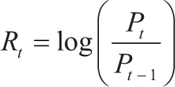
To ensure the reliability of the results and avoid any spurious findings, we handle return values that have equal prices on consecutive days by replacing them with infinitesimally small values. This precautionary step prevents the utilization of null values in the prediction models, thereby maintaining the integrity of the analysis.

3.2.2. Time-Varying-Parameter-Vector-Autoregressive (TVP-VAR) Model

To assess the interconnectedness of returns among the target variables, we employ the TVP-VAR model, inspired by the work of Antonakakis and Gabauer (2017). The foundation for studying dynamic connectedness is put forth by Diebold and Ylmaz (2009, 2012, and 2014). The TVP-VAR methodology has a substantial advantage over earlier approaches because it does not require a set window size, which can produce inconsistent results dependent on selection bias. Because rolling windows prevent the loss of data points, this method also has the advantage of allowing for relatively small sample sizes. This makes it possible to comprehend the TVP-VAR model’s foundation for return connectedness in greater detail. We offer a more thorough explanation of the framework’s operation below to give a better understanding of how it functions. Equations 2 and 3 describe a TVP-VAR model:

Z_{t} = B_{t} Z_{t - 1} + ε_{t} \sim N (0, S_{t})

(2)

B_{t} = B_{t - 1} + v_{t} \sim N (0, R_{t})

(3)

where Z_t represents conditional volatilities vector dimension k * 1, Z_t _{– 1} is an k_p * 1 lagged conditional vector, B_t is an k * k_p dimensional time-varying coefficient matrix, and ε_t is an k * 1 dimensional error disturbance vector with a k * k dimensional time varying variance-covariance matrix, S_t . The parameter B_t depends on their own lag values B_{t –} ₁ and on k * k_p dimensional error matrix with an k_p * k_p variance-covariance matrix.

After reviewing the contributions of Koop et al. (1996) and Pesaran and Shin (1998), the next stage involves computing the scaled generalized forecast error variance decomposition (GFEVD) based on an H-step forward forecast. Unlike the error decomposition variance technique employed by Diebold and Ylmaz (2009), which does call on the ordering of variables, the GFEVD is completely invariant to such considerations. Building on the methodology proposed by Diebold and Yilmaz (2014), the GFEVD is derived by transforming the TVP-VAR model into its vector moving average representation (TVP-VMA) using the Wold theorem. This transformation is achieved through the process in Equation 4:

Z_{t} = B_{i t} Z_{t - i} + ε_{t} = \sum_{j = 0}^{\infty} A_{j t} ε_{t - j}

(4)

To ensure consistency and facilitate interpretation, the unscaled GFEVD represented by $ϕ_{ij, t}^{g} (H)$ is normalized to obtain the scaled version. This normalization process ensures that the summation within each row of the matrix equals unity, as described by Equation 5. Consequently, we obtain $\tilde{ϕ_{ij, t}^{g} (H)},$ which represents the pairwise directional connectedness from variable j to variable i (see Equation (6)). This measure analyzes how much of an impact variable j has on variable i, taking into account its contribution to the forecast error variance. The computation of these terms involves the steps described in Equations (5) and (6):

ϕ_{ij, t}^{g} (H) = \frac{S^{- 1} \sum_{i = 1, i \neq j}^{H - 1} {({l^{'}}_{i} A_{t} S_{t} l_{j})}^{2}}{\sum_{j = 1}^{k} \sum_{i = 1, i \neq j}^{H - 1} ({l^{'}}_{i} A_{t} S_{t} {A^{'}}_{t} l_{i})}

(5)

\tilde{ϕ_{ij, t}^{g} (H)} = \frac{ϕ_{ij, t}^{g} (H)}{\sum_{j = 1}^{k} ϕ_{ij, t}^{g} (H)}

(6)

The selection vector, denoted as li, is defined such that its value is 1 for the index i and 0 elsewhere. The connectivity metrics are then developed using the paradigm suggested by Diebold and Yılmaz (2012, 2014) as described in Equations (7)–(10):

T O_{j t} = \sum_{i = 1, i \neq j}^{k} \tilde{ϕ_{ij, t}^{g} (H)}

(7)

F R O M_{j t} = \sum_{i = 1, i \neq j}^{k} \tilde{ϕ_{ji, t}^{g} (H)}

(8)

N E T_{j t} = T O_{j t} - F R O M_{j t}

(9)

T C I_{t} = k^{- 1} \sum_{j = 1}^{k} T O_{j t}

(10)

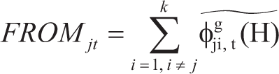
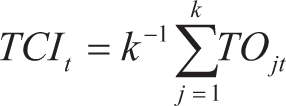
In this context, Equation (7) quantifies the total directional connectedness originating from variable j to all other variables within the network. Conversely, Equation (8) measures the total directional connectedness directed towards variable j from all other variables in the network. The net total direction of connectedness associated with variable j can be determined by taking the difference between Equations (7) and (8), which gives rise to Equation (9). Here, Equation (9) serves as an indicator of the overall net directionality of connectedness attributed to variable j within the network. Positive values in Equation (9) indicate that variable j has a greater influence on other variables than it receives from them, indicating a net outward direction of connectedness. Conversely, negative values suggest that variable j is more influenced by other variables in the network than it influences them, reflecting a net inward direction of connectedness. By considering Equation (9), we gain insights into the dominant direction and strength of the interconnectedness associated with variable j within the network. For example, if NET_jt > 0, it implies that the net driver status of variable j within the network can be inferred from this analysis, as it predominantly serves as a transmitter of shocks. This indicates that variable j plays a crucial role in shaping the dynamics of the network by propagating and influencing the transmission of shocks among the variables. An overall indicator of how related all of the network’s variables are is given by Equation (10). This measure acts as a proxy for determining the degree of interconnectivity and related market risk.

The Total Connectedness Index (TCI), which is derived from Equation (10), has a greater value when a shock in one variable has a significant effect on the entire network. This signifies greater market risk and increased connection. In such circumstances, a shock originating from a single variable might spread quickly, have a substantial impact on the network, and even cause significant market volatility. A lower TCI rating, on the other hand, denotes a considerably lesser degree of interconnectivity and related market risk. There is less of a chance for widespread volatility when a given variable gets a shock because the repercussions on other variables in the network are less noticeable. We can learn more about the market’s overall interconnection and risk profile by analyzing the TCI. We can determine how much a shock to one variable can affect the network as a whole, which is useful information for risk assessment and management. A higher TCI stresses the significance of carefully observing how variables are interconnected because it denotes a higher susceptibility to systemic dangers. A lower TCI, on the other hand, indicates a more robust and diverse market where shocks are less likely to spread widely throughout the network.

3.2.3. Spillover Index

The original Diebold and Yilmaz (2009) spillover measure, often known as the DY spillover index, which is developed from the idea of variance decomposition in an N-variable vector autoregression (VAR), is extended by this methodology. This technique goes further by measuring directional spillovers inside an extended VAR framework, whereas the DY framework primarily focuses on capturing total spillovers within a simple VAR framework, where the results might be affected by variable ordering through Cholesky factor orthogonalization. By using this approach, the possible influence of variable ordering on the outcomes is removed, producing more reliable and order-independent results.

Consider a covariance stationary N-variable VAR(p), $T y x_{t} = \sum_{i = 1}^{p} ϕ_{i} X_{t - i} + ϵ_{t},$ where $ϵ \sim (0, Σ)$ is a vector of independently distributed disturbances with identical distributions. The moving average representation is $x_{t} = \sum_{i = 0}^{\infty} A_{i} ϵ_{t - i},$ where the N * N coefficient matrices A_i obey the recursion A_i = Φ₁A_{i – 1} + Φ₂A_{i – 2} + … + Φ_pA_{i – p}, with A₀ being an N * N identity matrix and with A_i = 0 for i < 0. Understanding the dynamics of the system depends on its moving average coefficients (or transformations such as impulse response functions or variance decompositions). We use variance decompositions, which break down each variable’s forecast error variance into components that can be attributed to different system shocks. We can evaluate the proportion of the H step-ahead error variance in forecasting x_i that is attributable to shocks to x, for all j ≠ i, for each i, using the variance decompositions. Orthogonal innovations must typically be assumed in order to calculate variance decompositions. The VAR model innovations in this instance, though, are contemporaneously correlated. Through identification strategies such as Cholesky factorization, orthogonality is attained; however, this imposes a dependence on the ordering of the variables in the variance decompositions. We use the generalized VAR framework, often known as KPPS, developed by Koop et al. (1996) and Pesaran and Shin (1998) to address this problem. Variance decompositions produced by this approach are independent of variable ordering. The generalized VAR framework accepts correlated shocks while properly accounting for them using the observed historical distribution of errors, in contrast to methods that seek to orthogonalize shocks. Because the shocks for each variable are not orthogonalized, the row total of the items in the variance decomposition table, which represents the sum of contributions to the prediction error variance, may or may not be equal to one.

We define the own variance shares as the proportion of the H-step-ahead error variances in forecasting x_i that can be attributed to shocks specifically affecting x_i, for i = 1, 2, …, N. On the other hand, cross variance shares, or spillovers, refer to the proportions of the H-step-ahead error variances in forecasting x_i that can be attributed to shocks affecting other variables x_j, for i, j = 1, 2, …, N such that i ≠ j. We represent the KPPS H-step-ahead forecast error variance decompositions as $θ_{i j}^{g} (H)$ for H = 1, 2, …, and this is described in Equation (11).

θ_{i j}^{g} (H) = \frac{σ_{j j}^{- 1} \sum_{h = 0}^{H - 1} {({e^{'}}_{i} A_{h} Σ e_{j})}^{2}}{\sum_{h = 0}^{H - 1} ({e^{'}}_{i} A_{h} Σ {A^{'}}_{h} e_{i})}

(11)

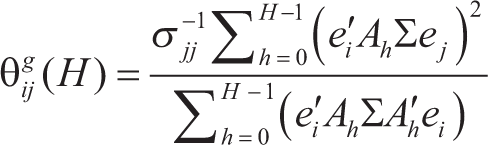
In this context, Σ represents the variance matrix for the error vector ε, σ_ij denotes the standard deviation of the error term for the jth equation, and e_i is the selection vector, with a value of one in the ith element and zeros elsewhere. As previously mentioned, it is important to note that the sum of the elements in each row of the variance decomposition table does not equal to $\sum_{j = 1}^{N} θ_{i j}^{g} (H) \neq 1 .$ To utilize the information provided by the variance decomposition matrix for calculating the spillover index, each entry in the variance decomposition matrix is normalized by dividing it by the sum of its respective row, as indicated in Equation (12):

\tilde{θ_{i j}^{g} (H)} = \frac{θ_{i j}^{g} (H)}{\sum_{j = 1}^{N} θ_{i j}^{g} (H)}

(12)

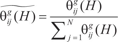
By employing the volatility contributions obtained from the KPPS variance decomposition, the calculation of the total volatility spillover index is performed using Equation (13):

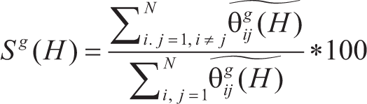
S^{g} (H) = \frac{\sum_{i . j = 1, i \neq j}^{N} \tilde{θ_{i j}^{g} (H)}}{\sum_{i, j = 1}^{N} \tilde{θ_{i j}^{g} (H)}} * 100

(13)

Examining the total volatility spillover index offers valuable insights into the magnitude of volatility shocks transmitted among significant asset classes. However, to gain a more profound understanding of the specific directions of volatility spillovers, we employ the generalized VAR approach. This approach encompasses generalized impulse responses and variance decompositions, enabling us to overcome the issue of variable ordering. By utilizing this methodology, we calculate directional spillovers by considering the normalized elements of the generalized variance decomposition matrix. We use Equation (14) to calculate the directional volatility spillovers that market i receives from all other markets j:

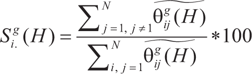
S_{i .}^{g} (H) = \frac{\sum_{j = 1, j \neq 1}^{N} \tilde{θ_{i j}^{g} (H)}}{\sum_{i, j = 1}^{N} \tilde{θ_{i j}^{g} (H)}} * 100

(14)

The directional volatility spillovers from market i to all other markets j are measured similarly, as shown in Equation (15):

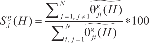
S_{. i}^{g} (H) = \frac{\sum_{j = 1, j \neq 1}^{N} \tilde{θ_{j i}^{g} (H)}}{\sum_{i, j = 1}^{N} \tilde{θ_{j i}^{g} (H)}} * 100

(15)

The set of directional spillovers (as shown in Equation (15)) can be thought of as a decomposition of all spillovers, highlighting those coming from (or going to) a particular source. According to Equation (16), we determine the net volatility spillovers from market i to all other markets j:

S_{i}^{g} (H) = S_{. i}^{g} (H) - S_{i .}^{g} (H)

(16)

By measuring the difference between the gross volatility shocks sent to and received from all other markets, the net volatility spillover is determined. This measure provides a concise summary of the contribution, of how much each market contributes, net, to the volatility seen in other markets. Examining the net pairwise volatility spillovers, which are defined as given in Equation (17), is also beneficial in addition to the net volatility spillover.

S_{i j}^{g} (H) = (\frac{\tilde{θ_{j i}^{g} (H)} - \tilde{θ_{i j}^{g} (H)}}{N}) * 100

(17)

By deducting the gross volatility shocks transmitted from market i to market j from the shocks transmitted from market j to market i, it is possible to determine the net pairwise volatility spillover between markets i and j. This measure quantifies the net directional flow of volatility between the two markets, capturing the extent to which each market influences the volatility of the other.

4. Results

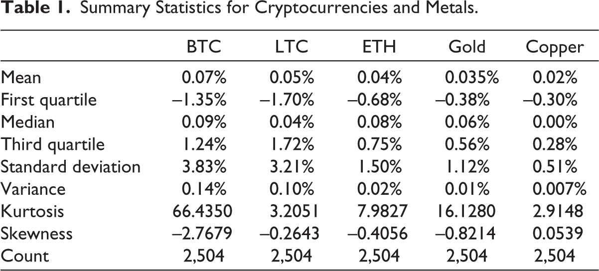
The results of our investigation on the connectedness and spillover dynamics between cryptocurrencies and metals are presented in this section. Table 1 provides a thorough overview of the summary information.

The average daily returns for the three cryptocurrencies and the two metals over a 10-year period are shown in Table 1 along with some additional information. It shows that Gold, Litecoin, Ethereum, and Bitcoin have the highest average returns. This shows that investing in cryptocurrency has been more lucrative recently. It is crucial to remember that cryptocurrencies also display more volatility, which denotes higher risk (as seen by the standard deviation and variance in Table 1). In order to mitigate this risk, less risky assets might be used, which could, however, lead to reduced profits. From a portfolio optimization standpoint, it would be intriguing to examine whether combining a diverse range of cryptocurrencies with metals in a portfolio can yield portfolios with both low risk and high rewards over a 10-year timeframe.

Table 1.

Summary Statistics for Cryptocurrencies and Metals.

	BTC	LTC	ETH	Gold	Copper
Mean	0.07%	0.05%	0.04%	0.035%	0.02%
First quartile	–1.35%	–1.70%	–0.68%	–0.38%	–0.30%
Median	0.09%	0.04%	0.08%	0.06%	0.00%
Third quartile	1.24%	1.72%	0.75%	0.56%	0.28%
Standard deviation	3.83%	3.21%	1.50%	1.12%	0.51%
Variance	0.14%	0.10%	0.02%	0.01%	0.007%
Kurtosis	66.4350	3.2051	7.9827	16.1280	2.9148
Skewness	–2.7679	–0.2643	–0.4056	–0.8214	0.0539
Count	2,504	2,504	2,504	2,504	2,504

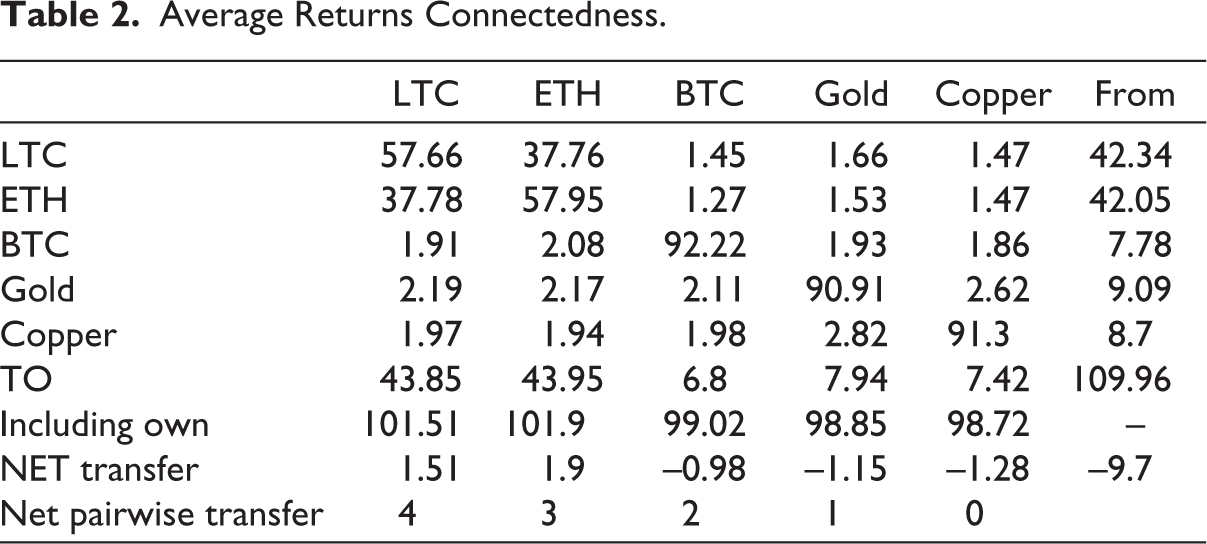
Next, we present the outcomes of the TVP-VAR connectedness analysis. Table 2 showcases the results for the Average Connectedness across assets. Table 2 presents the estimated contribution to the variance of forecast errors for metal i resulting from disruptions to metal j, as indicated by the ijth entry. The off-diagonal elements represent the rates of spillovers, whereas the diagonal elements represent self-induced return spillovers. The last column reveals that Ethereum and Litecoin exhibit the highest level of connectedness in this context. Interestingly, despite Bitcoin’s popularity and high trading volume, the evidence suggests that it is less connected compared with other cryptocurrencies. Moreover, Ethereum’s connectedness is primarily contributed by Litecoin, followed by Gold and Copper. This finding supports the motivation for this study, indicating that cryptocurrencies and metals have experienced back-and-forth movement due to major economic and financial events over the past decade, driven by factors such as high returns, low volatility, and risk hedging. Additionally, we observe that Gold is more connected than Copper among metals. This could be attributed to the fact that Gold offers both low risk and high returns, whereas Copper, although relatively more stable, does not provide the same level of returns as Gold. Therefore, for investors shifting from cryptocurrencies to other assets, Gold appears to be a more attractive option when seeking stability without compromising significantly on returns. Furthermore, we calculate the Net Partial Dynamic Connectedness measures on a rolling basis, and the results are presented in Table 2.

Table 2.

Average Returns Connectedness.

	LTC	ETH	BTC	Gold	Copper	From
LTC	57.66	37.76	1.45	1.66	1.47	42.34
ETH	37.78	57.95	1.27	1.53	1.47	42.05
BTC	1.91	2.08	92.22	1.93	1.86	7.78
Gold	2.19	2.17	2.11	90.91	2.62	9.09
Copper	1.97	1.94	1.98	2.82	91.3	8.7
TO	43.85	43.95	6.8	7.94	7.42	109.96
Including own	101.51	101.9	99.02	98.85	98.72	–
NET transfer	1.51	1.9	–0.98	–1.15	–1.28	–9.7
Net pairwise transfer	4	3	2	1	0

A visual examination presented in Figure 1 confirms the findings obtained from the TVP-VAR connectedness analysis. We observe that Litecoin and Ethereum exhibit high connectedness with each other as well as with metals. In contrast, although there is some evidence of Bitcoin being connected with other assets, this connection is notably weaker when compared to other cryptocurrencies. Notably, Copper and Gold demonstrate higher levels of connectedness compared with other pairs such as Bitcoin-Copper and Litecoin-Gold. This suggests a potential association in investment behavior between Gold and Copper.

Figure 1.

Net Pairwise Dynamic Connectedness for Cryptocurrencies and Metals.

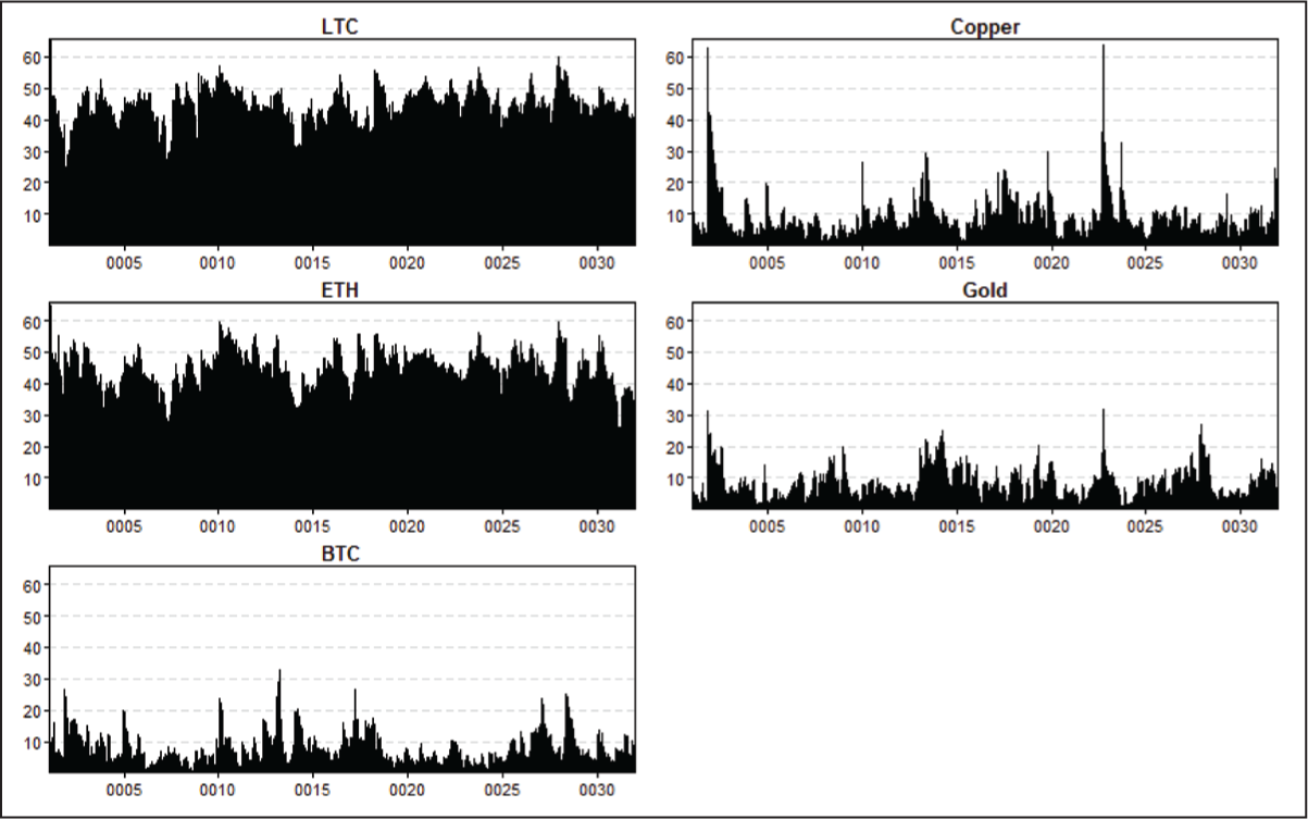
The examination of the Dynamic to Total Directional Connectedness plot depicted in Figure 2 reinforces the previous findings. Litecoin and Ethereum exhibit evidence of high connectedness, supporting the conclusions drawn from earlier analyses. Interestingly, contrary to previous findings, the plot suggests that Bitcoin and Gold demonstrate comparable levels of connectedness. Additionally, Copper displays relatively higher connectedness levels compared with both Bitcoin and Gold. Furthermore, the pairwise connectedness index (PCI) supports similar conclusions, further validating the findings obtained thus far (see Figure 3). The analysis reveals that the Litecoin-Ethereum pair exhibits the highest PCI among all pairs studied. The results for other pairs are consistent with the findings discussed earlier, further supporting the robustness of the analyses conducted.

Figure 2.

Dynamic to Total Directional Connectedness for Cryptocurrencies and Metals.

Figure 3.

Pairwise Connectedness Index (PCI) for Cryptocurrencies and Metals.

In accordance with the approach introduced by Diebold and Yilmaz (2012), we compute the Spillover Index metric.

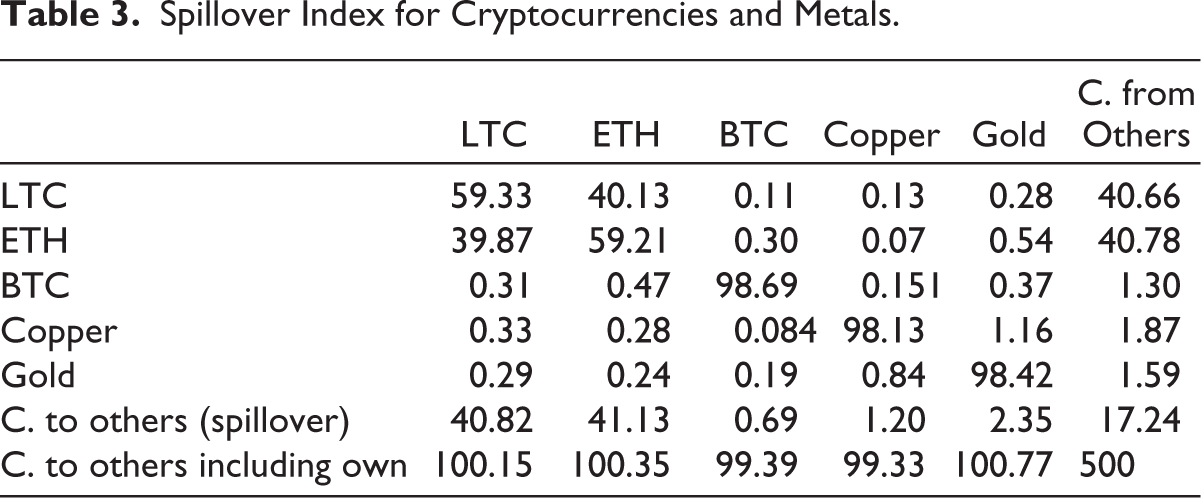
In Table 3, the last column and the last two rows present measures of connectedness, which further strengthen our initial observations. Specifically, Litecoin and Ethereum exhibit higher levels of connectedness compared with Bitcoin. From a risk transfer standpoint, Copper receives a greater level of risk from other assets compared with Gold. Additionally, it is evident that Copper transfers more volatility to Gold than the other way around. This finding has practical implications, as it suggests that investments in base metals can potentially serve as effective hedges against fluctuations in bullion volatility. Moreover, Litecoin transfers more volatility to Ethereum than vice versa, indicating that Litecoin, when compared solely with Ethereum, demonstrates better risk transfer properties. As we have previously observed, Litecoin has a higher average return over the 10-year investment horizon (2013–2022). Thus, the evidence from our analyses supports the notion that Litecoin can be considered a safer and more profitable cryptocurrency compared with Ethereum, although Ethereum remains a preferable choice in terms of volatility or standard deviation of returns.

Table 3.

Spillover Index for Cryptocurrencies and Metals.

	LTC	ETH	BTC	Copper	Gold	C. from Others
LTC	59.33	40.13	0.11	0.13	0.28	40.66
ETH	39.87	59.21	0.30	0.07	0.54	40.78
BTC	0.31	0.47	98.69	0.151	0.37	1.30
Copper	0.33	0.28	0.084	98.13	1.16	1.87
Gold	0.29	0.24	0.19	0.84	98.42	1.59
C. to others (spillover)	40.82	41.13	0.69	1.20	2.35	17.24
C. to others including own	100.15	100.35	99.39	99.33	100.77	500

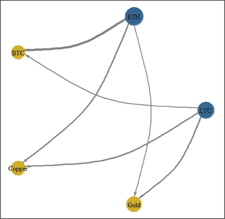
These outcomes can also be summarized and visualized in the network representation provided in Figure 4. Figure 4 illustrates the network of assets based on Net Spillovers. The network highlights that Ethereum and Litecoin act as net transmitters of volatility to Gold, Copper, and Bitcoin. On the other hand, in spite of its popularity, Bitcoin shows little evidence of a risk-transmission relationship with any of these metals.

Figure 4.

Network Based on Net Spillovers.

5. Conclusion

This article provides a systematic examination of the dynamics of interconnection between two metals and three cryptocurrencies. By analyzing the effects of return and volatility spillovers, the primary goal is to look at how interconnected the market is. In order to do this, we use the TVP-VAR method, which Antonakakis and Gabauer (2017) used to measure return spillovers. In addition, we calculate the amount of spillover using the Diebold and Yilmaz (2014) Spillover Index technique. The results of our investigation show that there is a strong relationship between Litecoin and Ethereum as well as these cryptocurrencies and metals. However, the link between Bitcoin and other assets is less strong than it is for other cryptocurrencies. Notably, Copper and Gold show a higher level of connection than couples such as Bitcoin-Copper or Litecoin-Gold, pointing to a probable relationship between Gold and Copper’s investment behavior. The significant degree of connectivity between Litecoin, Ethereum, and metals suggests that these markets may be interdependent and share certain traits. When developing investing strategies using these assets, these findings have consequences for analysts and investors. The linkages between Gold and Copper that have been identified also point to a possible association between investment behavior, which may affect risk management and portfolio diversification strategies.

Understanding the shock transmitters and receivers inside the metals network is crucial for investors. They may assess the possible effects of internal risks related to these markets using this useful knowledge, and they can create the best methods for risk management and portfolio optimization. The study’s conclusions can be a great resource for hedging choices including both metals and cryptocurrency. The need of proactive portfolio management for these assets is highlighted by the changing nature of return spillovers, as demonstrated by the examples of Gold and Copper (Balcilar et al., 2021). Our results emphasize the need for investors to actively monitor and modify their portfolios in light of changing dynamics and the directionality of spillovers among metals.

The implications of our analysis can help domestic investors better comprehend the risks and opportunities in the metals market. They are more prepared to manage risk, optimize their portfolios, and employ hedging techniques thanks to this knowledge, which eventually results in more effective and specialized investment methods. A thorough understanding of the risk dynamics that influence the interactions within the metal markets depends on the conclusions of the net volatility spillover effects and return connectedness. These findings provide insightful information that can help create a strategy for managing and reducing market risks. These insights would be especially useful to policymakers, as they work to maintain market stability and put in place efficient risk management measures. Our analysis provides a useful tool to understand how emerging commodity markets interact with one another as well. Further, cryptocurrency and commodity markets often act as leading indicators for both foreign and domestic macroeconomic conditions. By analyzing the dynamics and interconnectedness of these markets, we can gain valuable insights into broader economic trends and developments. By studying the interconnectedness and volatility dynamics using this methodology, researchers and policymakers can gain valuable insights into the evolving landscape of these markets, which can inform decision-making processes and help anticipate potential economic trends.

Footnotes

Declaration of Conflicting Interests

The authors declared no potential conflicts of interest with respect to the research, authorship, and/or publication of this article.

Funding

The authors received no financial support for the research, authorship, and/or publication of this article.

References

Adekoya

O. B.

, & Oliyide

J. A.

(2021). How COVID-19 drives connectedness among commodity and financial markets: Evidence from TVP-VAR and causality-inquantiles techniques. Resources Policy, 70, 101898.

Antonakakis

, & Gabauer

(2017). Refined measures of dynamic connectedness based on TVP-VAR (MPRA Paper 78282). University Library of Munich.

Antonakakis

, Chatziantoniou

, & Gabauer

(2020). Refined measures of dynamic connectedness based on time-varying parameter vector autoregressions. Journal of Risk and Financial Management, 13(4), 84.

Antonakakis

, Chatziantoniou

, Floros

, & Gabauer

(2018a). The dynamic connectedness of UK regional property returns. Urban Studies, 55(14), 3110–3134.

Antonakakis

, Gabauer

, Gupta

, & Plakandaras

(2018b). Dynamic connectedness of uncertainty across developed economies: A time-varying approach. Economics Letters, 166, 63–75.

Awartani

, & Maghyereh

A. I.

(2013). Dynamic spillovers between oil and stock market in the gulf cooperation council countries. Energy Economics, 36, 28–42.

Balcilar

, Gabauer

, & Umar

(2021). Crude oil futures contracts and commodity markets: New evidence from a TVP-VAR extended joint connectedness approach. Resources Policy, 73, 102219.

Baruník

, & Kˇrehlík

(2018). Measuring the frequency dynamics of financial connectedness and systemic risk. Journal of Financial Econometrics, 16(2), 271–296.

Basher

S. A.

, Haug

A. A.

, & Sadorsky

(2018). The impact of oil-market shocks on stock returns in major oil-exporting countries. Journal of International Money and Finance, 86, 264–280.

10.

Billio

, Getmansky

, Lo

A. W.

, & Pelizzon

(2012). Econometric measures of connectedness and systemic risk in the finance and insurance sectors. Journal of Financial Economics, 104(3), 535–559.

11.

Bouri

, Cepni

, Gabauer

, & Gupta

(2021a). Return connectedness across asset classes around the COVID-19 outbreak. International Review of Finance Analysis, 73, 101646.

12.

Bouri

, Gabauer

, Gupta

, & Tiwari

A. K.

(2021b). Volatility connectedness of major cryptocurrencies: The role of investor happiness. Journal of Behavioral and Experimental Finance, 30, 100463.

13.

Bri₹ere

, Chapelle

, & Szafarz

(2012). No contagion, only globalization and flight to quality. Journal of International Money and Finance, 31(6), 1729–1744.

14.

Brière

, & Signori

(2012). Inflation-hedging portfolios: Economic regimes matter. The Journal of Portfolio Management, 38(4), 43–58.

15.

Chen

, & Tongurai

(2022). Spillovers and interdependency across base metals: Evidence from China’s futures and spot markets. Resources Policy, 75, 102479.

16.

Diebold

F. X.

, & Yilmaz

(2009). Measuring financial asset return and volatility spillovers with application to global equity markets. The Economic Journal, 119(534), 158–171.

17.

Diebold

F. X.

, & Yilmaz

(2012). Better to give than to receive: Predictive directional measurement of volatility spillovers. International Journal of Forecasting, 28(1), 57–66.

18.

Diebold

F. X.

, & Yılmaz

(2014). On the network topology of variance decompositions: Measuring the connectedness of financial firms. Journal of Econometrics, 182(1), 119–134.

19.

Dua

, & Tuteja

(2016). Financial crises and dynamic linkages across international stock and currency markets. Economic Modelling, 59, 249–261.

20.

Fassas

A. P.

(2020). Risk aversion connectedness in developed and emerging equity markets before and after the COVID-19 pandemic. Heliyon, 6(12), e05715.

21.

Ftiti

, Louhichi

, & Ben Ameur

(2021). Cryptocurrency volatility forecasting: What can we learn from the first wave of the COVID-19 outbreak? Annals of Operations Research, 1–26. 10.1007/s10479-021-04116-x

22.

Gabauer

(2021). Dynamic measures of asymmetric & pairwise connectedness within an optimal currency area: Evidence from the ERM I system. Journal of Multinational Financial Management, 60, 100680.

23.

Gabauer

, & Gupta

(2018). On the transmission mechanism of country-specific and international economic uncertainty spillovers: Evidence from a TVP-VAR connectedness decomposition approach. Economics Letters, 171, 63–71.

24.

Huang

, Li

, Zhang

, & Chen

(2021). The effects of uncertainty measures on commodity prices from a time-varying perspective. International Review of Economics Finance, 71, 100–114.

25.

, Bouri

, Roubaud

, & Shahzad

S. J. H.

(2018). Risk spillover between energy and agricultural commodity markets: A dependence-switching CoVaR-copula model. Energy Economics, 75, 14–27.

26.

Kang

S. H.

, McIver

, & Yoon

S. M.

(2017). Dynamic spillover effects among crude oil, precious metal, and agricultural commodity futures markets. Energy Economics, 62, 19–32.

27.

Kayal

, & Balasubramanian

(2021). Excess volatility in bitcoin: Extreme value volatility estimation. IIM Kozhikode Society & Management Review, 10(2), 222–231.

28.

Kayal

, & Maheswaran

(2021). A study of excess volatility of gold and silver. IIMB Management Review, 33(2), 133–145.

29.

Kayal

, & Rohilla

(2021). Bitcoin in the economics and finance literature: A survey. SN Business & Economics, 1(7), 88.

30.

Koop

, Pesaran

M. H.

, & Potter

S. M.

(1996). Impulse response analysis in non-linear multivariate models. Journal of Econometrics, 74, 119–147.

31.

Madichie

C. V.

, Ngwu

F. N.

, Eze

E. A.

, & Maduka

O. D.

(2023). Modelling the dynamics of cryptocurrency prices for risk hedging: The case of Bitcoin, Ethereum, and Litecoin. Cogent Economics & Finance, 11(1), 2196852.

32.

Mandacı

P. E.

, Cagli

E. Ç.

, & Taşkın

(2020). Dynamic connectedness and portfolio strategies: Energy and metal markets. Resources Policy, 68, 101778.

33.

Mensi

, Shafiullah

, Vo

X. V.

, & Kang

S. H.

(2021). Volatility spillovers between strategic commodity futures and stock markets and portfolio implications: Evidence from developed and emerging economies. Resources Policy, 71, 102002.

34.

Murty

, Victor

, & Fekete-Farkas

(2022). Is bitcoin a safe haven for Indian investors? A GARCH volatility analysis. Journal of Risk and Financial Management, 15(7), 317.

35.

Nair

J. V.

, & Kayal

(2022). A study of tail-risk spillovers in cryptocurrency markets. Global Business Review. 10.1177/09721509221079969

36.

Oztek

M. F.

, & Ocal

(2017). Financial crises and the nature of correlation between commodity and stock markets. International Review of Economics & Finance, 48, 56–68.

37.

Pesaran

H. H.

, & Shin

(1998). Generalized impulse response analysis in linear multivariate models. Economics Letters, 58(1), 17–29.

38.

Philippas

, & Siriopoulos

(2013). Putting the “C” into crisis: Contagion, correlations and copulas on EMU bond markets. Journal of International Financial Markets, Institution and Money, 27, 161–176.

39.

Reboredo

J. C.

, & Ugolini

(2016). The impact of downward/upward oil price movements on metal prices. Resources Policy, 49, 129–141.

40.

Som

, & Kayal

(2022). A multicountry comparison of cryptocurrency vs gold: Portfolio optimization through generalized simulated annealing. Blockchain: Research and Applications, 3(3), 100075.

41.

Song

, Bouri

, Ghosh

, & Kanjilal

(2021). Rare earth and financial markets: Dynamics of return and volatility connectedness around the COVID-19 outbreak. Resources Policy, 74, 102379.

42.

Umar

, Jareño

, & Escribano

(2021). Oil price shocks and the return and volatility spillover between industrial and precious metals. Energy Economics, 99, 105291.

43.

Varma

, Venkataramani

, Kayal

, & Maiti

(2021). Short-term impact of COVID-19 on Indian stock market. Journal of Risk and Financial Management, 14(11), 558.

44.

Wang

Y. S.

, & Chueh

Y. L.

(2013). Dynamic transmission effects between the interest rate, the US dollar, and gold and crude oil prices. Economic Modelling, 30, 792–798.

45.

Wen

, & Wang

(2021). Volatility linkages between stock and commodity markets revisited: Industry perspective and portfolio implications. Resources Policy, 74, 102374.

46.

Zhang

, & Broadstock

D. C.

(2020). Global financial crisis and rising connectedness in the international commodity markets. International Review of Financial Analysis, 68, 101239.