Decentralization and Its Impact on Growth in India

Abstract

We study the effect of revenue decentralization (RD) and expenditure decentralization (ED) on sub-national growth in India from 1981–1982 to 2015–2016 for 14 large (non-special-category) states. Our study provides evidence that both RD and ED play a defining role in India’s sub-national growth in this three-and-a-half-decade period. We use a panel data model with fixed effects (FE) and Driscoll and Kraay standard errors that control for heteroscedasticity, autocorrelation and cross-sectional dependence. To test for causality between growth and decentralization, we use the Granger non-causality test. The regression analysis is supplemented with the distribution dynamics approach. We find that: (a) While decentralization Granger-caused economic growth, the reverse causality effect of growth on decentralization was not significant; (b) Economic growth increased significantly after liberalization; (c) Decentralization, capital expenditure and social expenditure had significant positive impacts on economic growth; and (d) States that had high levels of decentralization also had high levels of per capita income, while states that had low decentralization also exhibited low per capita income.

Keywords

Decentralization in India economic growth sub-national government distribution dynamics Granger Causality

Introduction

Growth economics has identified several factors, such as technology (Arrow, 1962; Romer, 1990; Solow, 1956), innovation (Grossman & Helpman, 1991), human capital (Barro, 1991; Becker, 1993), capital deepening (Kuznets, 1973), regional policies (Krugman, 1991), social and political institutions (Asher & Novosad, 2017; Deshpande, 2011; North, 1987), inequality (Alesina & Perotti, 1996; Deaton & Drèze, 2002) and public policy (Easterly, 2019), which impact income dynamics.

A different strand of literature explaining regional growth has pointed out that in a federal structure, it is possible to influence sub-national growth by reallocating expenditure and revenue responsibilities between different tiers of government (Davoodi & Zou, 1998). It has been argued in the same vein that greater democratization and devolution of powers could positively impact both the efficiency and effectiveness of economic policies (Feruglio, 2007). Therefore, an identical set of policies in a country may differ in effectiveness across different states due to the variations in institutional and organizational factors across states (Sala-i-Martin, 1996). Allocation of fiscal functions among different government tiers, depending on their comparative advantage, leads to better governance and economic efficiency (Oommen, 2006). The reason this may occur is that fiscal decentralization could improve the delivery of public services, as well as revenue collection (Kalirajan & Otsuka, 2012). Therefore, a better understanding of the extent and process of decentralization in a country may be vital to enhancing regional growth.

Decentralization is defined as the devolution of revenue, expenditure and decision-making authority to democratically elected lower-level governments, mostly independent of the central government (World Bank, 2000). Theoretically, three necessary conditions are required for decentralized provision of public goods and services to be Pareto-superior: heterogeneity, externalities and economies of scale. Welfare is maximized in a decentralized set-up when regions are heterogeneous in their preferences for public goods and services. Decentralization is considered beneficial when regions do not show evidence of interregional spillovers of the benefits of their expenditure to other regions and when there is no cost saving through uniform, centralized provision of public goods and services (Oates, 1972).

Fiscal decentralization enhances efficiency in usage of local resources for several reasons, as local governments are directly associated with the beneficiaries of these policies (Ebel & Yilmaz, 2002; RBI, 2006). Sub-national governments may be subject to greater scrutiny by the public, since they are closer to them in a decentralized set-up. Public scrutiny forces authorities to appoint competent staff and to undertake efficient expenditure. Decentralization can reduce moral-hazard and agency problems and reduce the number of bureaucracy layers (Boadway & Shah, 2007).

With fiscal decentralization, regional governments can provide public services based on the preferences of their respective constituencies in contrast to the central government (Weingast, 2014). Besides, these regional and local governments face competition from their counterparts, leading to the efficient provision of public services (Oates, 1999). These policies could impact not only growth but also inequality (Clements et al., 2015).

There are some potential risks associated with decentralization as well. Some economists have associated decentralization with slower growth, leading to macroeconomic instability (Prud’homme, 1995). Fiscal decentralization, if not done correctly, can widen regional inequalities, can have an adverse effect on the fiscal balances and can lead to coordination failures among sub-national governments and the centre (Hindricks et al., 2008; Rodden et al., 2003; World Bank, 2002). In order to realize the benefits of fiscal decentralization, it is essential that sub-national governments be able to undertake autonomous expenditure decisions and be accountable for them. Similarly, governments should have adequate revenue to undertake their spending responsibilities either through sufficient taxation autonomy or steady unconditional transfers (Hankla, 2008).

The jury is out on the impact of decentralization on economic growth. While some studies show that decentralization had a positive impact on economic growth (Akai & Sakata, 2002; Justin & Zhiqiang, 2000; Qiao et al., 2008), others have found that fiscal decentralization had a negative impact on economic growth (Davoodi & Zou, 1998; Jin, 2009; Zhang & Zou, 1998). The impact of fiscal decentralization differs from country to country and over time and would depend on the institutional economic structure of the economy.

The Indian Context

The Indian Constitution is federal in its set-up. However, from the 1950s till the 1980s, the fiscal power was mainly concentrated with the central government. It was only in 1991 that the states were given greater powers to follow their economic and social policies (Bagchi, 2003). In 1992, constitutional recognition was given to the third-tier level of government in India. Our study is restricted to the analysis of decentralization at the sub-national (state) level due to the unavailability of data at the local (third-tier) level for the time period of our study. While India has undertaken expenditure decentralization (ED) to the sub-national governments, it has still not achieved much in terms of tax devolution (Panda et al., 2019).

Multiple types of explanations have been used to understand India’s sub-national growth trajectory (Ahluwalia, 2000; Lolayekar & Mukhopadhyay, 2020; Raju, 2012; Sachs et al., 2002). However, data limitations have restricted the covariates that similar international studies have employed (Maiti & Marjit, 2015; Nayyar, 2008). For example, disaggregated data on investments and savings, interstate trade data, research and development expenditure are not available at the state level. While literacy rates could serve as a proxy to human capital, they are available only with decadal periodicity after the population census (Census, 2011).

There has been a varying degree of decentralization across regions in India. Concerning delivery of public services and mobilization of resources, both physical and human, some states have been more successful than others (Rao, 2008). With decentralization, it has been argued, the local elites have been in a position to have greater control over a larger share of public resources than the poor, which has implications for inequality (Drèze & Sen, 1995). Others have found that decentralization has fostered development equitably across states through health and education expenditures (Kalirajan & Otsuka, 2012). Therefore, apart from growth, decentralization also has a distributional impact.

We examine these issues in our study that spans the last three and a half decade (from 1981–1982 to 2015–2016). During this period, the Indian economy saw significant institutional changes, with increased open market policies from the early 1990s (Kotwal et al., 2011) and the 73rd and 74th constitutional amendments devolving more powers to lower tiers of government (Rao, 2002). In India, an increase in capital expenditure simultaneous with a decrease in revenue expenditure (without affecting the fiscal deficit) was found to have a positive influence on the economic growth (RBI, 2016). The capital outlay of state governments was considered growth-inducing and had a more prolonged effect on the economy than revenue expenditure (Jain & Kumar, 2013). Social sector expenditures (including expenditures on education and health) are also significant for India’s growth and development (Mittal, 2016). These expenditures enhance economic growth by positively influencing the competitiveness, productivity and efficiency of labour and reducing absolute poverty. Further, sustainable economic growth requires social sustainability, and social expenditures could help achieve that (Kaur et al., 2013). Ganaie et al. (2018) found a positive impact of ED but a negative impact of revenue decentralization (RD) on economic growth.

We contribute to this literature by using a twofold strategy. First, we use a regression model to establish the impact of decentralization on growth. We use a panel fixed effects (FE) model with both ED and RD as covariates, along with social and capital expenditures (Devarajan et al. 1996). We also use the Dumitrescu and Hurlin (2012) Granger non-causality test to confirm causality between growth and decentralization. Second, we complement the regression-based approach with a distribution dynamics approach proposed by Quah (1997). This approach overcomes problems that could arise from the non-fulfilment of the normality assumption in regression-based approaches. More importantly, it can help better identify the presence of convergence clubs and polarization among states (Kar et al., 2011; Lolayekar & Mukhopadhyay, 2017).

We find that RD and ED had a positive impact on growth. Similarly, capital expenditure and social expenditure had a significant positive impact on economic growth, which was higher after liberalization. This has significant implications for public policy relating to the devolution of powers among different tiers of government in India. These findings also add to the growth and public finance literature.

The rest of the article is organized as follows. In the second section, we present the materials and methods. In the third section, we present the results, followed by the analysis in the fourth section. We conclude the article in the fifth section with a discussion of our findings and their policy implications.

Materials and Methods

The theoretical framework used to analyse the influence of fiscal decentralization on economic growth is the commonly used production–function approach (Davoodi & Zou, 1998).

As a first step, we define the quantitative measure of decentralization used in this study to measure the effects on income. Many cross-country studies in the past have measured fiscal decentralization as the ratio of sub-national government expenditure/revenue to total government expenditure/revenue (Ebel & Yilmaz, 2002). This measure may overestimate the extent of decentralization and can misrepresent the impact of fiscal decentralization on major economic indicators. The more recent trend is to construct measures of fiscal decentralization which reflect the sub-national governments’ autonomy in terms of both expenditure and revenue decisions (Akai & Sakata, 2002). Hence, it is necessary to subtract that expenditure from the sub-national-government share mandated by the central government or undertaken on behalf of the central government. Expenditure financed through conditional transfers whose use is predetermined by the centre is deducted from the sub-national expenditure. Again, in terms of revenue, it is necessary to distinguish between own revenue, shared taxes and transfers. In terms of the RD measure, only those resources over which the sub-national government has authority in terms of either the tax rate or the tax base are included.

We have constructed two measures of decentralization: expenditure and revenue. The ED variable measures the extent of autonomy a state enjoys in its expenditure vis-à-vis the centre. ED is measured by estimating the ratio of the ‘i-th’ state’s expenditure as a proportion of its total expenditure (centre plus state). This measure is adopted from Qiao et al. (2008) and modified suitably to measure the decentralization level of Indian states. We use per capita measures to control for heterogeneity in population across states. The state’s own expenditure does not include the central grants, and the formula used is as follows:

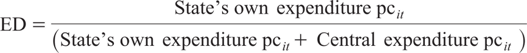
E D = \frac{S t a t e ’ s o w n \exp ​ e n d i t u r e p c_{i t}}{(S t a t e ’ s o w n \exp ​ e n d i t u r e p c_{i t} + C e n t r a l \exp ​ e n d i t u r e p c_{i t})}

(1)

where

State’s own expenditure pc_it = state’s aggregate expenditure minus central grants to the state in per capita terms;

Central expenditure pc_it = central grants per capita, including grants under the central plan schemes, centrally sponsored schemes, state plan schemes and non-plan grants;

i = ith state; and

t = time period.

Although the state government undertakes state plan schemes, we excluded the grants to states under these schemes, as state governments do not have autonomy in their spending decisions. One of the reasons cited for terminating the Planning Commission in 2014 through which these grants to state plan schemes were provided was to increase the autonomy of states and promote cooperative federalism among states (Rao, 2016).

The RD variable measures the extent of autonomy a state enjoys in its revenues vis-à-vis the centre. This represents the ability of the ‘ith’ state to raise its own revenues through taxes. We measure this by estimating the ratio of the ‘ith’ state’s tax revenue as a proportion of its total revenue (centre plus state). Therefore, the state’s own tax revenue excludes the state’s share in central taxes, as the state has no control over the tax rate or base in terms of revenue collection. This measure is adopted from Oommen (2006) and modified suitably to measure decentralization at the sub-national level. The formula used is as follows:

RD = state’s own tax revenue per capita (pc) of state ‘i’ divided by the sum of aggregate central tax revenue per capita and state’s own tax revenue per capita.

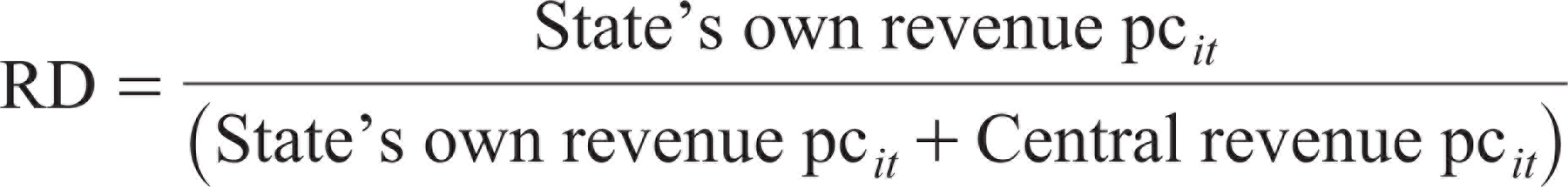
R D = \frac{S t a t e ’ s o w n r e v e n u e p c_{i t}}{(S t a t e ’ s o w n r e v e n u e p c_{i t} + C e n t r a l r e v e n u e p c_{i t})}

(2)

where

State’s own revenue pc_it = states’ own tax revenue in per capita terms.

Central revenue pc_it = contribution of the central funds to the ‘ith’ state.

Here, central revenue per capita is the state’s share in central taxes of the ‘ith’ state in per capita terms, i = ith state, and t = time period.

Regression-based Approach

We examine the impact of ED and RD on state-level growth using the commonly used regression method with a formal econometric model. We anticipate that growth is subject to many influences apart from fiscal decentralization, such as population, human capital, initial per capita GDP, the real investment share in GDP, total labour force, the degree of openness of economy/volume of trade, the inﬂation rate and policy reforms (Feltenstein & Iwata, 2005; Lin & Liu, 2000; Zhang & Zou, 1998). The tax rate has also been used as an explanatory variable (Davoodi & Zou, 1998; Zhang & Zou, 1998). Expenditures on health, economic development, administration and education (as a ratio of total state-government spending) have been used as control variables while determining the impact of decentralization on GDP growth (Zhang & Zou 2001). As a substitute for investment expenditure (for which data is not available at the sub-national level), we have used the government capital expenditure. In India, the crowding-out hypothesis and Ricardian-equivalence hypothesis have received mixed responses (Ghatak & Ghatak, 1996; Mitra, 2006; Pradhan et al., 1990), but there has been evidence of a positive correlation between private capital investment and public capital expenditure at the national level during certain phases (Bahal et al., 2018).

India undertook significant market reforms in the 1990s. The empirical growth literature often distinguishes economic policies between two periods: before 1990 and after 1990. We, therefore, wish to account for this structural change before and after the liberalization process. The conceptual model we propose predicts growth as an outcome of these factors (see Equation [3]).

\begin{matrix} G r o w t h = f (c a p i t a l \exp ​ e n d i t u r e, s o c i a l \exp ​ e n d i t u r e, \\ e c o n o m i c p o l i c y, d e c e n t r a l i z a t i o n) \end{matrix}

(3)

The specific linear model used for estimation is stated in Equation (4):

\begin{matrix} \ln P C I_{i t} = β_{1} + β_{2} S o c i a l E x p_{i t} + β_{3} C a p i t a l E x p_{i t} + β_{4} L i b_{i t} + β_{5} D e c_{i t} + \\ β_{6} (s q_D e c_{i t}) + a_{i} + e_{i t} \end{matrix}

(4)

where

i is the ith state;

t is the time period;

lnPCI is the natural log of gross state domestic product (GSDP) per capita at current prices;

CapitalExp is the proportion of capital outlay to the aggregate expenditure of state i at current prices;

SocialExp is the proportion of social expenditure to the aggregate expenditure of state i at current prices;

Lib is a dummy variable separating the post-liberalization period from the pre-liberalization period. It takes the value ‘0’ for pre-liberalization years (up to 1990) and ‘1’ after that (1991 onwards);

Dec is a measure of decentralization (ED for expenditure and RD for revenue);

sq_Dec is the square of the measure of decentralization (ED for expenditure and RD for revenue);

α is an entity-specific intercept (used in the FE model); and

e is the stochastic error term.

Panel data models enable researchers to analyse economic processes while considering the heterogeneity of units and accounting for dynamic effects that are not included in cross-sectional data (Greene, 2010). One advantage also is that they are more informative and provide greater variability in terms of the data collected and are thus more efficient in the estimation of parameters. These models enable researchers to analyse complex behavioural models that are subject to less restrictive assumptions (Ullah & Giles, 1998).

A basic method applied to panel data is the pooled ordinary least squares (POLS) model, also known as the population-averaged model (see Equation [4], where α_i = 0). POLS provide efficient estimates only when the classical model’s assumptions are satisfied, including zero conditional mean of error term, homoscedasticity, independence across units and strict exogeneity of independent variables. Such conditions are hard to fulfil, and if data is available, then researchers prefer panel data models, choosing between the random effects (RE) and FE models depending on the nature of the data. An RE model is resorted to when unobserved effects are not correlated with the explanatory variables. If this assumption is violated, the RE estimator will produce biased and inconsistent estimates (Greene, 2010). To solve this problem the within estimator or FE estimator is used. In this method, deviations from individual means are computed. Thus, even if a correlation between unobserved factors and some explanatory variables exists, the within estimator will produce unbiased and consistent estimates (Hausman & Taylor, 1981). Accordingly, in Equation (4), we would anticipate that β_i = 0 and α_i ≠ 0. We also use the Dumitrescu and Hurlin (2012) Granger non-causality test to analyse the two-way causality between growth and decentralization.

Testing for Causality

The popular test to analyse the causal relationship between time series variables was first proposed by Granger (1969). This was extended by Dumitrescu and Hurlin (2012) to analyse heterogenous, balanced panels and to test bidirectional causality. We tested whether decentralization causes growth (Equation [5]) and whether the causality runs from growth to decentralization (Equation [6]) using the following regression equations:

Δ \ln P C I_{i t} = α_{i} + \sum_{k = 1}^{K} β_{i k} Δ \ln P C I_{i, t - k} + \sum_{k = 1}^{K} γ_{i k} Δ D e c_{i, t - k} + Ε_{i t}

(5)

Δ D e c_{i t} = α_{i} + \sum_{k = 1}^{K} β_{i k} Δ D e c_{i, t - k} + \sum_{k = 1}^{K} γ_{i k} Δ \ln P C I_{i, t - k} + Ε_{i t}

(6)

where:

Lag order k is assumed to be identical for all panels;

coefficients (β, γ) are allowed to differ across individuals but are assumed to be time-invariant; and

Δ stands for the first difference of the stationary variables.

A precondition to running the Granger causality test is that the variables be stationary. We used the Hadri Lagrange multiplier (LM) test to test for unit roots in our panel data. This test is suitable for data with a large T and a moderate N and balanced panel models, like the one we use for our study. While the variables were not stationary at level, they were found to be stationary when we used their first difference. For all the three variables (lnPCI, ED and RD), we could not reject the null hypothesis, meaning that all the panels were stationary at the first difference (Table 3).

Next, we undertook the Dumitrescu and Hurlin (2012) Granger non-causality test using the first difference of the lnPCI and decentralization variables. We used the Z-bar test for interpreting the results, as according to Hurlin and Dumitrescu (2012), it is suitable for our data with large time periods and few panels.

We ran two separate regressions for decentralization: model 1 for ED and model 2 for RD (see Table 2). In keeping with earlier contributions (Akai & Sakata, 2002; Hanif et al., 2020; Yushkov, 2015), we decided to run separate models with ED and RD, as the covariates had a significant correlation between them (the correlation coefficient value was 0.72). The correlation between the fiscal variables CapitalExp and SocialExp, on the other hand, was found to be low (correlation coefficient value was 0.11). We, therefore, did not anticipate the problem of multicollinearity arising if we kept both the fiscal variables in the regression estimation. Since our data took the form of a balanced panel, we could use either a POLS or a panel data model (FE or RE).

In the model with ED as a predictor (model 1), we used the Breusch–Pagan LM (BP-LM) test to choose between the RE and POLS models. The results (Prob. > chi-square = 0.000) suggested that the RE model would be preferred over the POLS. We next chose between the RE model and the FE model. Usually, we would have used the Hausman test to determine this. Since we used robust standard errors to avoid problems of heteroscedasticity, the preferred test then was the Sargan–Hansen test as a substitute for the Hausman test (Baum et al., 2014). The post-estimation test rejected the null hypothesis of RE, implying that the RE model would provide inconsistent estimates. The FE model was, therefore, the preferred option. In RD (model 2), the BP-LM test suggested that the POLS model was preferred to the RE model. Hence, we used the F-test to choose between the POLS and FE models. The results indicated that the FE model would be preferred over the POLS model (Prob. > F = 0.000). Therefore, in both the ED and RD models, the FE model was the preferred choice. Also, in both these models, the post-estimation tests indicated: (a) the presence of heteroscedasticity among the variables (modified Wald test in the FE model); (b) the presence of serial correlation—first-order autocorrelation (Wooldridge test); and (c) the presence of cross-sectional correlation between panels (BP-LM test for independence).

Three popular methods address the problem of heteroscedasticity, autocorrelation and cross-sectional dependence for long panel data (large T and small N) (Hoechle, 2007). The first method is the Parks-Kmenta method. This method is applied to panel data using a feasible generalized least square (FGLS)-based algorithm, but it produces unacceptably small standard errors. To overcome this problem, Beck and Katz (1995) proposed the estimation of POLS with panel-corrected standard errors. The third method produces the Driscoll and Kraay (DK) standard errors, which can be applied to POLS/weighted least squares (WLS) and FE (within) estimations. The DK standard errors are not only consistent in the presence of heteroscedasticity and auto-correlation but are also robust to general levels of cross-sectional correlation (Fofanah, 2020; Fuinhas et al., 2019; Hartwell, 2014; Simionescu et al., 2016).

Distribution Dynamics Approach

This approach encompasses both time series and cross-section properties of the data simultaneously. The density of distribution ϕ_t evolves as per Equation (7):

φ_{t} = M \cdot φ_{t - 1}

(7)

where M maps the transition between the income distributions for two consecutive periods, ‘t’ and ‘t - 1’. This is a first-order Markov process, as the density distribution ϕ for the period ‘t’ only depends on the density ϕ for the immediately preceding period ‘t - 1–. In our estimates below, we have assumed that the distribution ϕ has a finite number of states.

In estimating the dynamics of income distribution, there are three possibilities for an economy’s behaviour over a given period of time:

It may move ahead;

It may stay where it was; or

It may even fall behind.

The distribution dynamics information is encoded in a transition probability matrix (TPM). This is a square matrix that describes the probabilities of moving from one state to another in a dynamic system. Each row represents the probability of moving from the state represented by that row to the other states. All entries have a value between 0 and 1, which represents probability, and the sum of the entries’ values in a row adds up to 1. Here, the evolution of income is modelled as a Markov process governed by a transition probability. The current state (in a first-order Markov chain) only depends on the immediate previous state (Kemeny, 2003). The advantage of this methodology is that it formulates a law of motion for the entire distribution of incomes between the periods under analysis, allowing us to model the existence of convergence clubs in the data. In the case of transition probability matrix, it is assumed that an economy or region over a given time period (say, 1 year or 5 years) either remains in the same position or changes its relative position in the income distribution (Bandyopadhyay, 2012; Quah, 1996).

For the Markov transition matrices, we assume that the probability of variable s_t taking a particular value depends only on its previous value s_t-1 according to the first-order Markov chain:

P {s_{t} = j | s_{t - 1} = i} = P_{i j}

(8)

where P_ij indicates the probability that state i will be followed by state j and the sum of values in each row will add up to 1:

P_{i 1} + P_{i 2} + \dots + P_{i n} = 1

(9)

The transition matrix constructed is as follows:

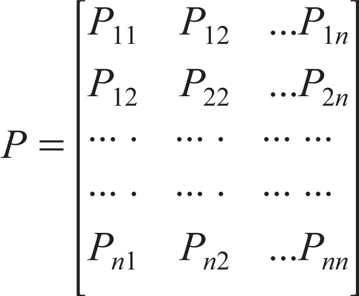
P = [\begin{matrix} P_{11} P_{12} \dots P_{1 n} \\ P_{12} P_{22} \dots P_{2 n} \\ \dots . \dots . \dots \dots \\ \dots . \dots . \dots \dots \\ P_{n 1} P_{n 2} \dots P_{n n} \end{matrix}]

(10)

where row i and column j indicate the probability that state i will be followed by state j.

The Markov chains model the evolution of relative income distribution. We thus identify the position of the economy in the starting period. This is done by dividing the income distribution into ‘income states’ over a range of income levels. We then observe how many of the economies that are in an income state, say between 0.75 and 1 in the initial period, remain in that same state (persistence) or shift elsewhere in the next period (mobility). The TPM measures the probability of the income level in a country or region rising, falling or remaining unchanged between two periods (Magrini, 2007).

Data

We use data for 14 large general-category (also called non-special-category) states of India. The special- and general-category states differ significantly in terms of their own revenue generation, cost disabilities and central financial assistance and hence cannot be compared in terms of fiscal decentralization (FC, 2009; Rao, 2017). Hence, the special-category states have been left out of this study. We have also not included the states like Goa and Delhi in the analysis, because these are outliers in per capita income terms and have a comparatively small population. The period for the study is 1981–1982 to 2015–2016, which is the largest time span for which data is currently available for all variables under consideration.

We combine data from multiple sources. GSDP per capita data is taken from MOSPI (various years). GSDP data from 1980–1981 to 1992–1993 is based on the 1981 series, data from 1993–1994 to 1998–1999 is based on the 1993–1994 series, data from 1999–2000 to 2003–2004 is based on the 1999–2000 series, data from 2004–2005 to 2010–2011 is based on the 2004–2005 series, and finally data from 2011–2012 to 2015–2016 is based on the 2011–2012 series. Data on all types of state expenditures, state revenues and central transfers to states are taken from the (EPWRF various years). All the data used in our study are at current prices.

The state-level year-wise population estimates are obtained by interpolating decadal census estimates to obtain the states’ annual population from 1981–1982 to 2015–2016 (PC, 2014). The newly formed states (Jharkhand, Uttarakhand, Chhattisgarh and Telangana) have been merged with their respective original states (Bihar, Uttar Pradesh, Madhya Pradesh and Andhra Pradesh) for analytical comparability.

Results

We first present the summary statistics of the variables used in the regression analysis (Table 1). The 35-year period with 14 states generates 490 observations. LnPCI has a mean of 9.58 (overall) and has a standard deviation of 1.26 (overall). While ED has a mean of 0.9, RD has a mean of 0.69, confirming that India is much more decentralized in expenditure than in revenue. However, RD has a higher variation as compared to ED. The capital expenditure ratio has a mean of 0.11, and the social expenditure ratio has a mean of 0.31.

Table 1.

Summary Statistics of Variables of 14 States (from 1981–1982 to 2015–2016)

Variable		Mean	Std. Dev.	Min.	Max.
LnPCI	Overall	9.58	1.259	7.110	12.12
	Between		0.363	8.824	10.02
	Within		1.209	7.348	11.90
ED	Overall	0.90	0.042	0.726	0.97
	Between		0.034	0.827	0.94
	Within		0.026	0.800	0.98
RD	Overall	0.69	0.151	0.286	0.93
	Between		0.153	0.376	0.87
	Within		0.031	0.593	0.78
CapitalExp	Overall	0.11	0.047	–0.032	0.22
	Between		0.028	0.056	0.14
	Within		0.038	0.005	0.20
SocialExp	Overall	0.31	0.046	0.165	0.43
	Between		0.030	0.234	0.35
	Within		0.036	0.186	0.42

Source: Data on all types of state expenditures, revenues and transfers: (EPWRF, various years). Data on PCI: (MOSPI, various years).

Note: Observations—N = 490, n = 14, T = 35.

We present the regression results (including those of the Granger causality regression), followed by the analysis of the distribution dynamics approach.

The results of the regression Equation (4) are presented in Table 2. ED and RD both were found to have a significant and positive influence on lnPCI, confirming that a reallocation of expenditure shares and revenue collection responsibilities to the states will enhance growth. Moreover, this could be achieved without altering the aggregate government spending/revenue. A unit increase in RD will lead to a 4.81% increase in lnPCI. ED, on the other hand, was found to have a non-linear relationship with lnPCI, and therefore the extent of the impact of ED would depend on the value of ED at which change is being contemplated.

Table 2.

Fixed Effects Regression Using Driscoll–Kraay Standard Errors, with Dependent Variable LnPCI

Variable	1 (ED)	2 (RD)
ED	53.15**
Sq_ED	–31.28*
RD		4.81**
CapitalExp	5.32***	5.71***
SocialExp	5.01*	5.65**
Lib	2.18***	2.115***
Constant	–16.56*	2.34
Within R-squared	0.688	0.698
F-statistic	F(5, 34) = 16.19	F(4, 34) = 22.50
F-statistic (p-value)	0.000	0.000
Sargan–Hansen statistic (p-value)	0.000
Breusch–Pagan Lagrange multiplier (LM) test	0.000	1.00
F-test that all u_i = 0		Prob. > F = 0.000
Modified Wald test (p-value)	0.000	0.000
Wooldridge test (p-value)	0.000	0.000
Breusch–Pagan LM test of independence (p-value)	0.000	0.000
No. of observations (maximum lag length 3)	490	490

Source: Authors’ calculations.

Note: ***, ** and * Significant at the 1%, 5% and 10% levels, respectively.

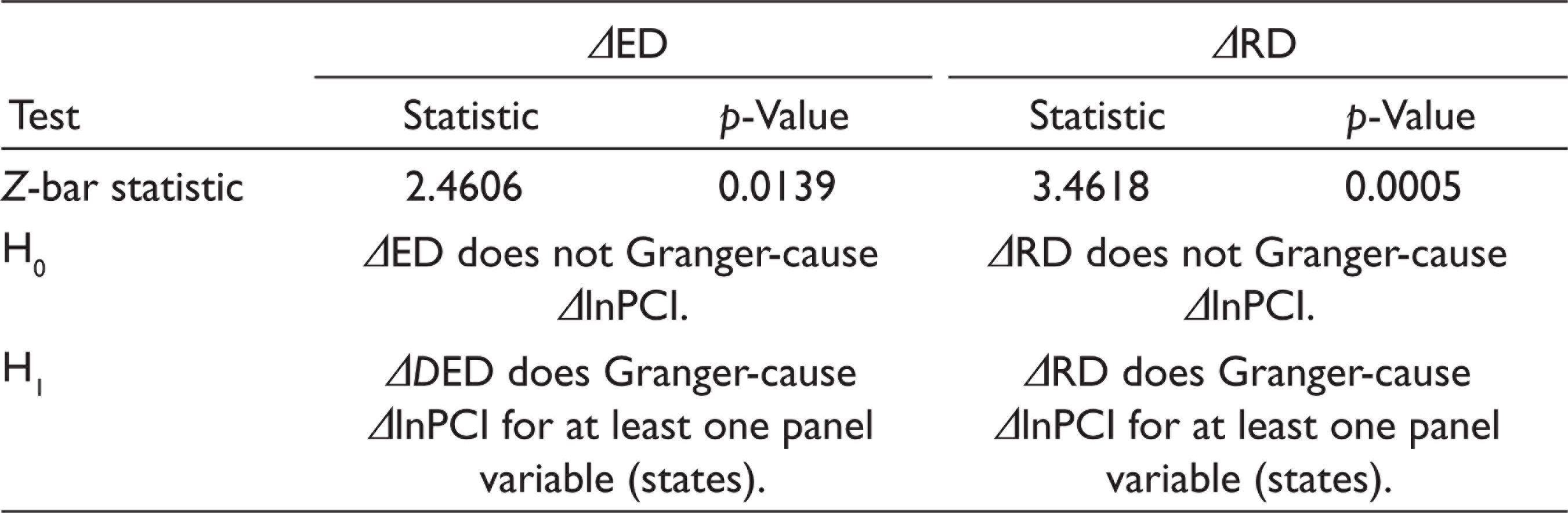
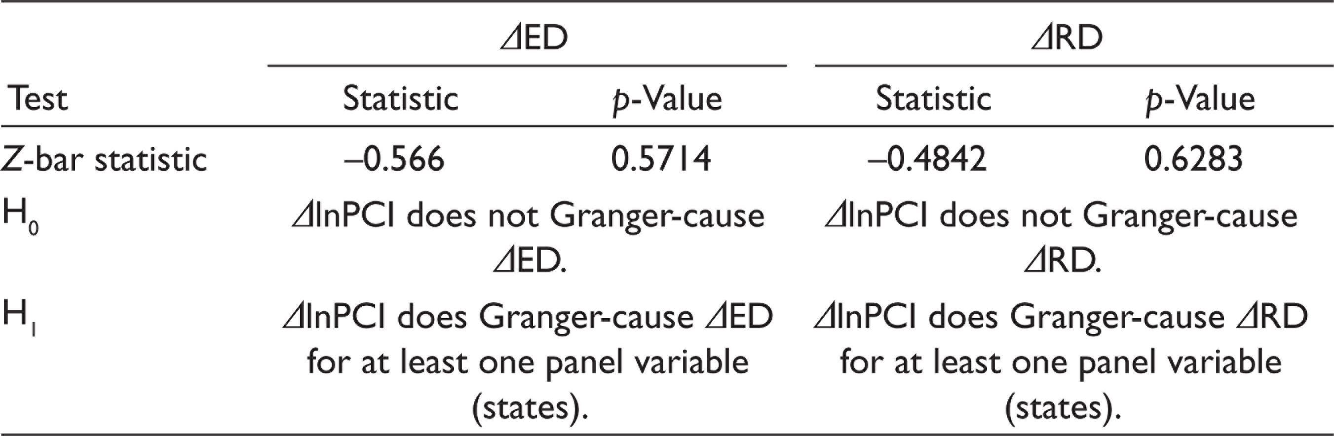
Social expenditure, as expected, was found to have a significant and positive influence on lnPCI in both regressions, confirming its importance for economic growth. Similarly, capital expenditure was also found to have a significant and positive influence on lnPCI. The liberalization variable was highly significant and positive, confirming the higher income growth in the post-liberalization phase in both the models. The R-squared (within) was around 0.69 for both the regression models and demonstrated the significance of estimates in the joint test of the hypothesis. Next, we discuss the results of the Dumitrescu and Hurlin (2012) Granger non-causality test. We find that in the case of ED and RD, we can reject the null hypothesis which states that ED/RD does not Granger-cause lnPCI and accept the alternative hypothesis that ED/RD does Granger-cause lnPCI for at least one of the states (Table 4 ).

Table 3.

Hadri Lagrange Multiplier Test for Unit Root in Panel Data

Test Statistic	ΔED		ΔRD		ΔlnPCI
Test Statistic	Statistic	p-Value	Statistic	p-Value	Statistic	p-Value
z	–0.8238	0.795	–0.0484	0.5193	–0.7724	0.795
Ho	All panels are stationary.
Ha	Some panels contain unit roots.

Source: Authors’ calculations.

Note: Number of panels (N) = 14; number of periods (T) = 34.

LR variance: Bartlett kernel, 5 lags.

Cross-sectional means removed.

Asymptotics: N, T  infinity sequentially.

Table 4.

Dumitrescu and Hurlin (2012) Granger Non-causality Test (decentralization  ΔlnPCI)

Test	ΔED		ΔRD
Test	Statistic	p-Value	Statistic	p-Value
Z-bar statistic	2.4606	0.0139	3.4618	0.0005
H₀	ΔED does not Granger-cause ΔlnPCI.		ΔRD does not Granger-cause ΔlnPCI.
H₁	ΔDED does Granger-cause ΔlnPCI for at least one panel variable (states).		ΔRD does Granger-cause ΔlnPCI for at least one panel variable (states).

Source: Authors’ calculations.

Note: Optimal number of lags (AIC) = 8 (lags tested = 1–8)

We also examined the bidirectional causality between lnPCI and decentralization. We found that while lnPCI does not Granger-cause decentralization, RD and ED do (Table 5).

Table 5.

Dumitrescu and Hurlin (2012) Granger Non-causality Test (ΔlnPCI  decentralization)

Test	ΔED		ΔRD
Test	Statistic	p-Value	Statistic	p-Value
Z-bar statistic	–0.566	0.5714	–0.4842	0.6283
H₀	ΔlnPCI does not Granger-cause ΔED.		ΔlnPCI does not Granger-cause ΔRD.
H₁	ΔlnPCI does Granger-cause ΔED for at least one panel variable (states).		ΔlnPCI does Granger-cause ΔRD for at least one panel variable (states).

Source: Authors’ calculations.

Note: Optimal number of lags (AIC) = 1 (lags tested = 1–7).

Analysis

We now examine how decentralization has affected the distribution of growth in incomes across states (see Table 6)—how many states remain in the same state and how many move elsewhere during this period. If they have moved above the diagonal, then the relative performance has been good, and if they have moved below the diagonal, the relative performance has been lacking. This allows us to create a distribution of states based on their performance during the two periods.

Table 6.

Relative Per Capita Income Transition Dynamics, 1981–2015

		2015
1981		States with an ending level less than 1.00	States with an ending level greater than 1.00	Number of states
	States with a starting level less than 1.00	Bihar, Madhya Pradesh, Odisha, Rajasthan, West Bengal	Andhra Pradesh, Karnataka, Uttar Pradesh, Kerala, Tamil Nadu	10
	States with a starting level greater than 1.00		Gujarat, Maharashtra, Haryana, Punjab	4

Source: Authors’ calculations.

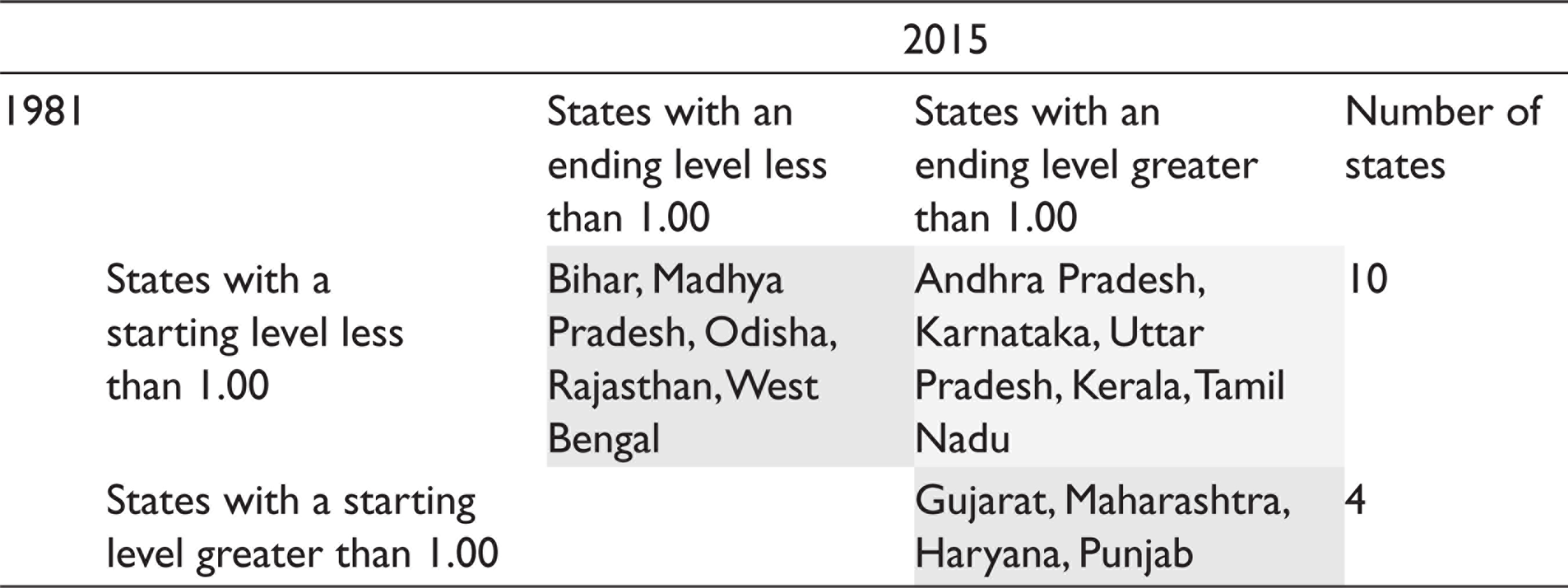
We use a 2 × 2 matrix to examine the mobility of states in PCI from 1981–1982 to 2015–2016. Five states (Andhra Pradesh, Karnataka, Uttar Pradesh, Kerala and Tamil Nadu) started with a PCI less than the national average but by 2015–2016 had moved above the national average (above the diagonal). Five states (Bihar, Madhya Pradesh, including Chhattisgarh, Odisha, Rajasthan and West Bengal) began with a PCI below the national average and ended in 2015–2016 below the national average. Four states (Gujarat, Maharashtra, Haryana and Punjab) began and ended with a PCI higher than the national average.

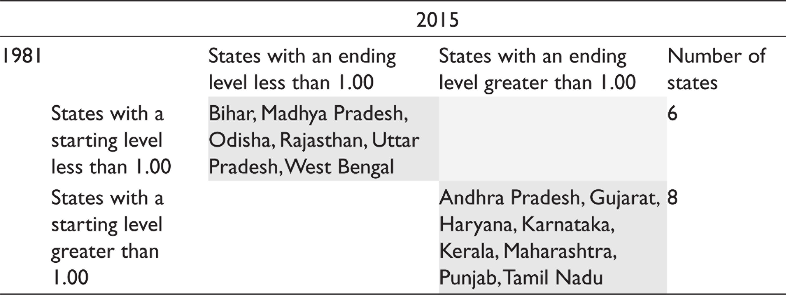
We now examine the degree of decentralization (expenditure and revenue). The transition matrices indicate heterogeneity in the degree of decentralization (see Table 7). Six states began the period with an RD lower than the average (Bihar, Madhya Pradesh, Odisha, Rajasthan, Uttar Pradesh and West Bengal), and eight states began with an RD higher than the average (Andhra Pradesh, Gujarat, Haryana, Karnataka, Kerala, Maharashtra, Punjab and Tamil Nadu). All these states maintained their relative positions, and there was no transition in RD during this period.

Table 7.

Relative Revenue Decentralization Transition Dynamics, 1981–2015

		2015
1981		States with an ending level less than 1.00	States with an ending level greater than 1.00	Number of states
	States with a starting level less than 1.00	Bihar, Madhya Pradesh, Odisha, Rajasthan, Uttar Pradesh, West Bengal		6
	States with a starting level greater than 1.00		Andhra Pradesh, Gujarat, Haryana, Karnataka, Kerala, Maharashtra, Punjab, Tamil Nadu	8

Source: Authors’ calculations.

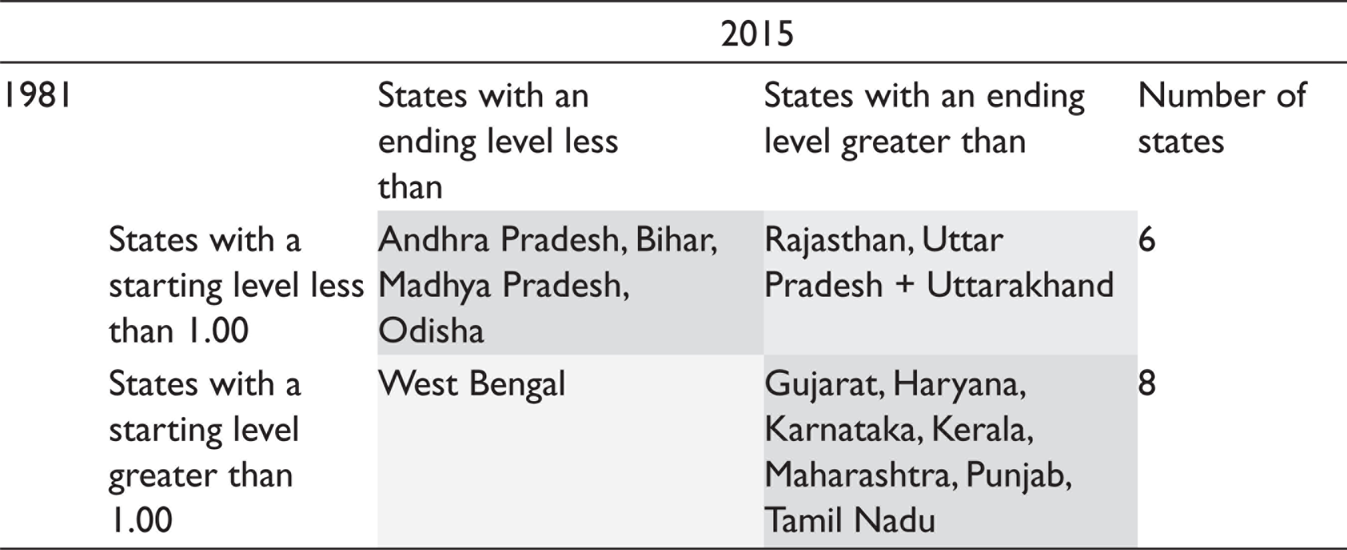
We find a higher transition among states in ED (see Table 8). Two states (Rajasthan and Uttar Pradesh) began with an ED lower than the national average and ended with an ED greater than the average. West Bengal was the only state that started with an ED greater than the average but ended with an ED lower than the average. Four states (Andhra Pradesh, Bihar, Madhya Pradesh and Odisha) began with an ED lower than the average and ended with an ED lower than the average. Seven states (Gujarat, Haryana, Karnataka, Kerala, Maharashtra, Punjab and Tamil Nadu) began with an ED greater than the average and ended with an ED greater than the average.

Table 8.

Relative Expenditure Decentralization Transition Dynamics, 1981–2015

		2015
1981		States with an ending level less than	States with an ending level greater than	Number of states
	States with a starting level less than 1.00	Andhra Pradesh, Bihar, Madhya Pradesh, Odisha	Rajasthan, Uttar Pradesh + Uttarakhand	6
	States with a starting level greater than 1.00	West Bengal	Gujarat, Haryana, Karnataka, Kerala, Maharashtra, Punjab, Tamil Nadu	8

Source: Authors’ calculations.

Four states (Gujarat, Maharashtra, Haryana and Punjab) began with a high PCI and ended with a high PCI. These four states exhibited high RD and ED in both the beginning and the end. Kerala and Tamil Nadu also had high ED and RD like the above four states and transitioned from an initial low PCI to a high PCI. Andhra Pradesh, Rajasthan and Uttar Pradesh are exceptions in different ways. Andhra Pradesh had a high RD but had a low ED (beginning and end) and could transition from a low PCI to a high PCI. Uttar Pradesh, on the other hand, had a low RD (beginning and end) but transitioned from a low ED to a high ED and was able to transition from a low PCI to a high PCI. Rajasthan shared the same status as Uttar Pradesh but could not make PCI gains as Uttar Pradesh did. West Bengal became part of those states that began and ended with a low PCI. It had a low RD (beginning and end), and its ED reduced between the two periods. All the states (Bihar, Madhya Pradesh and Odisha) that had a low ED and RD (beginning and end) also had a low PCI (beginning and end).

We visualize the association between decentralization and PCI spatially by creating four categories—corresponding to the four cells of the 2 × 2 matrix. If the ED, RD and PCI of a state are all in the first cell (less than average), then the state takes a value of ‘1’. If the ED, RD and PCI are in the fourth cell (all above the average), then the state takes a value of ‘4’. If PCI is higher than the average but either RD or ED is less than the average, then the state takes a value of 3. Similarly, if either RD or ED is less than the average but PCI is also below the national average, the state takes a value of 2. In Figure 1, the dark-blue areas have the lowest decentralization level and growth, while the red areas have high decentralization and a high PCI. The orange areas have one aspect of high decentralization (either ED or RD) but a high PCI. The light-blue areas have a low PCI and one aspect of high decentralization (either ED or RD). As we can see, in 2015–2016, the red areas have spread along the west coast and the orange areas in the south-east. The western segment, which was deep blue, has changed to light blue, but eastern India has remained blue and, in one case, has receded.

Figure 1.

Source: Github (2020) and Authors’ calculations.

Conclusion and Discussion

Our results show a positive impact of ED, as well as RD, on economic growth. Additionally, we find that: (a) ED has a non-linear relationship with economic growth; and (b) RD has a linear relationship with growth. This contrasts with some earlier studies that found a positive impact of ED but a negative impact of RD on economic growth (Ganaie et al., 2018). We also find that social sector expenditure and capital expenditure by the government have a positive impact on growth.

We used a twofold strategy to examine the research questions. A regression-based approach confirmed the direction of causality, as well as the significance of each of the covariates. We also used an alternative to the regression-based approach—the distributional dynamics approach—that did not capture causality but: (a) overcame the normality requirement for regression analysis; and (b) displayed the income distribution change using the Markov chain analysis.

Our results imply that by increasing the efficiency of resource allocation between the levels of government, it is possible to increase growth. Sub-national governments are better aware of the local needs and thus are in a better position to match local demand with the available resources. This can be achieved by increased devolution of expenditure and revenue raising responsibilities among the sub-national governments. Therefore, fiscal autonomy enhances growth. Besides this, the liberalization dummy variable, which was used to capture the structural change in the Indian economy, was found to have a significant and positive influence on growth.

Policy Implications

The findings of our study have important policy implications. The constitutional bodies of the central and state finance commissions, apart from their primary objective of fixing state shares, must also look at their role as being catalytic to economic growth. State governments that wish to expand their growth prospects should consider enhancing their decentralization efforts, infrastructure and social sector involvement. Our results also reiterate what is already well known in the growth literature: human capital enhances growth—thus, social expenditures have a positive influence on sub-national growth (Kalirajan & Otsuka, 2012).

In India, there has been wide diversity in the extent of decentralization, especially between third-tier governments. Many states have made very limited devolution of fiscal powers despite the constitutional provisions being available since the 73rd and 74th constitutional amendments in 1992. While our article has not looked at the third-tier level of government, we anticipate that further decentralization would not only strengthen local governance but may also enhance growth (Panagariya et al., 2014; Rao, 2008).

Footnotes

Declaration of Conflicting Interests

The authors declared no potential conflicts of interest with respect to the research, authorship and/or publication of this article.

Funding

The authors received no financial support for the research, authorship and/or publication of this article.

References

Ahluwalia

(2000). Economic performance of states in post-reforms period. Economic and Political Weekly, 35(19), 1637–1648.

Akai

, & Sakata

(2002). Fiscal decentralization contributes to economic growth: Evidence from state-level cross-section data for the United States. Journal of Urban Economics, 52, 93–108.

Alesina

, & Perotti

(1996). Income distribution, political instability, and investment. European Economic Review, 40(6), 1203–1228. https://doi.org/doi:10.1016/0014-2921(95)00030-5

Arrow

K. J.

(1962). The economic implications of learning by doing. The Review of Economic Studies, 29(3), 155. https://doi.org/10.2307/2295952

Asher

, & Novosad

(2017). Politics and local economic growth: Evidence from India. American Economic Journal: Applied Economics, 9(1), 229–273. https://doi.org/10.1257/app.20150512

Bagchi

(2003). Rethinking federalism: Changing power relations between the center and the states. Emerging Federal Process in India, 33(4), 21–42.

Bahal

, Raissi

, & Tulin

(2018). Crowding-out or crowding-in? Public and private investment in India (NCAER Working Papers 114). National Council of Applied Economic Research.

Bandyopadhyay

(2012). Convergence club empirics: Evidence from Indian states. In Bishop

J. A.

, & Salas

(Eds.), Inequality, mobility, and segregation: Essays in honor of Jacques Silber (pp. 175–203). Emerald Publishing.

Barro

R. J.

(1991). Economic growth in a cross section of countries. The Quarterly Journal of Economics, 106(2), 407. https://doi.org/10.2307/2937943

10.

Baum

, Connolly

, & O’Connor

(2014). Test of overidentifying restrictions after xtreg, xtivreg, xtivreg2 and xthtay. Faculty Microcomputer Resource Centre. https://fmwww.bc.edu/repec/bocode/x/xtoverid.html

11.

Beck

, & Katz

J. N.

(1995). What to do (and not to do) with time-series cross-section data. American Political Science Review, 89(3), 634–647. https://doi.org/10.2307/2082979

12.

Becker

G. S.

(1993). Human capital: A theoretical and empirical analysis, with special reference to education (3rd ed.). The University of Chicago Press.

13.

Boadway

, & Shah

(2007). Intergovernmental fiscal transfers principles and practice, public sector accountability and governance series. The International Bank for Reconstruction and Development, World Bank.

14.

Census (2011). Primary census abstract, office of the registrar general and census commissioner. Government of India Census 2011.

15.

Clements

B. J.

, de Mooij

R. A.

, Gupta

, & Keen

(Eds.). (2015). Inequality and fiscal policy. International Monetary Fund.

16.

Davoodi

, & Zou

H.-F.

(1998). Fiscal decentralization and economic growth: A cross country study. Journal of Urban Economics, 43, 244–257.

17.

Deaton

, & Drèze

(2002). Poverty and inequality in India: A reexamination (Working Paper No. 107). Centre for Development Economics, Delhi School of Economics.

18.

Deshpande

(2011). The grammar of caste: Economic discrimination in contemporary India. Oxford University Press.

19.

Devarajan

, Swaroop

, & Zou

H.-F.

(1996). The composition of public expenditure and economic growth. Journal of Monetary Economics, 37, 313–344.

20.

Drèze

, & Sen

(1995). India, economic development and social opportunity. Oxford University Press.

21.

Dumitrescu

, & Hurlin

(2012). Testing for granger non-causality in heterogeneous panels. Economic Modelling, 29(4), 1450–1460.

22.

Easterly

(2019). In search of reforms for growth: New stylized facts on policy and growth outcomes (No. w26318). National Bureau of Economic Research. https://doi.org/10.3386/w26318

23.

Ebel

R. D.

, & Yilmaz

(2002). On the measurement and impact of fiscal decentralization. The World Bank.

24.

EPWRF (various years). State finances. Economic and Political Weekly Research Foundation. www.epwrf.res.in

25.

FC (2009). Thirteenth finance commission report (2010–2015). Finance Commission of India.

26.

Feltenstein

, & Iwata

(2005). Decentralization and macroeconomic performance in China: Regional autonomy has its costs. Journal of Development Economics, 76(2), 481–501.

27.

Feruglio

(2007). Fiscal decentralization: An overview (Chapter 1). World Bank. https://www.google.com/url?sa=t&source=web&rct=j&url=http://siteresources.worldbank.org/PSGLP/Resources

28.

Fofanah

(2020). Effects of exchange rate volatility on trade: Evidence from West Africa. Journal of Economics and Behavioural Studies, 12(3), 32–52.

29.

Fuinhas

J. A.

, Marques

A. C.

, Koengkan

, Santiago

, & Couto

A. P.

(2019). The energy-growth nexus within oil production and oil rents context. Revista de Estudos Sociais, 21(42), 161. https://doi.org/10.19093/res7857

30.

Ganaie

A. A.

, Bhat

S. A.

, Kamaiah

, & Khan

N. A.

(2018). Fiscal decentralization and economic growth: Evidence from Indian states. South Asian Journal of Macroeconomics and Public Finance, 7(1), 83–108.

31.

Ghatak

, & Ghatak

(1996). Budgetary deficits and Ricardian equivalence: The case of India, 1950–1986. Journal of Public Economics, 60(2), 267–282. https://doi.org/10.1016/0047-2727(95)01551-5

32.

GITHUB (2020). India state map. https://github.com/datameet/maps/tree/master/States

33.

Granger

C. W.

(1969). Investigating causal relations by econometric models and cross spectral methods. Econometrica, 37(3), 424–438.

34.

Greene

(2010). Models for panel data. http://people.stern.nyu.edu/wgreene/Lugano2013/Greene-Chapter-11.pdf

35.

Grossman

G. M.

, & Helpman

(1991). Innovation and growth in the global economy. MIT Press.

36.

Hanif

, Wallace

, & Gago-de-Santos

(2020). Economic growth by means of fiscal decentralization: An empirical study for federal developing countries. SAGE Open, 10(4), 215824402096808. https://doi.org/10.1177/2158244020968088

37.

Hankla

C. R.

(2008). When is fiscal decentralization good for governance? The Journal of Federalism, 39(4), 632–650.

38.

Hartwell

C. A.

(2014). Do (successful) stock exchanges support or hinder institutions in transition economies? Cogent Economics and Finance, 2(946620). https://dx-doi-org.web.bisu.edu.cn/10.1080/23322039.2014.946620

39.

Hausman

J. A.

, & Taylor

W. E.

(1981). Panel data and unobservable individual effects. Econometrics, 49(6), 1377–1398.

40.

Hindricks

, Peralta

, & Weber

(2008). Competing in taxes and investment under fiscal equalization. Journal of Public Economics, 92(12), 2392–2402.

41.

Hoechle

(2007). Robust standard errors for panel regression with cross-sectional dependence. The Stata Journal, vv(ii), 1–31.

42.

Hurlin

, & Dumitrescu

(2012). Testing for granger non-causality in heterogeneous panels. HAL. http//halshs.archives-ouvertes.fr/halshs-00224434v2

43.

Jain

, & Kumar

(2013). RBI WPS(DEPR):07/2013: Size of government expenditure multipliers in India: A structural VAR analysis (RBI Working Paper Series No. 7). Reserve Bank of India. https://rbidocs.rbi.org.in/rdocs/Publications/PDFs/WP07180913F.PDF

44.

Jin

(2009). A comparative study of fiscal decentralization in China and India (Economic Dissertations). Department of Economics, Georgia State University. https://scholarworks.gsu.edu/cgi/viewcontent.cgi?article=1061&context=econ_diss

45.

Justin

, & Zhiqiang

(2000). Fiscal decentralization and economic growth in China. Economic Development and Cultural Change, 49. https://doi.org/10.1086/452488

46.

Kalirajan

, & Otsuka

(2012). Fiscal decentralization and development outcomes in India: An exploratory analysis. World Development, 40(8), 1511–1521. https://doi.org/10.1016/j.worlddev.2012.04.005

47.

Kar

, Jha

, & Kateja

(2011). Club-convergence and polarization of states: A nonparametric analysis of post-reform India. Indian Growth and Development Review, 4(1), 53–72. https://doi.org/10.1108/17538251111125007

48.

Kaur

, Misra

, & Suresh

A. K.

(2013). Cyclicality of social expenditures: Evidence from Indian states. Reserve Bank of India.

49.

Kemeny

J. G.

(2003). Markov chains. Pearson Education. https://www.aw-bc.com/greenwell/markov.pdf

50.

Kotwal

, Ramaswami

, & Wadhwa

(2011). Economic liberalization and Indian economic growth: What’s the evidence? Journal of Economic Literature, 49(4), 1152–1199. https://doi.org/10.1257/jel.49.4.1152

51.

Krugman

(1991). Increasing returns and economic geography. Journal of Political Economy, 99(3), 483–499. https://doi.org/10.1086/261763

52.

Kuznets

(1973). Modern economic growth: Findings and reflections. American Economic Review, 63(3), 247–258. https://ideas.repec.org/a/aea/aecrev/v63y1973i3p247-58.html

53.

Lin

J. Y.

, & Liu

(2000). Fiscal decentralization and economic growth in China. Economic Development and Cultural Change, 9(1), 1–21.

54.

Lolayekar

A. P.

, & Mukhopadhyay

(2017). Growth convergence and regional inequality in India (1981–2012). Journal of Quantitative Economics, 15(2), 307–328. https://doi.org/10.1007/s40953-016-0051-6

55.

Lolayekar

A. P.

, & Mukhopadhyay

(2020). Understanding growth convergence in India (1981–2010): Looking beyond the usual suspects. PLOS One, 15(6), e0233549. https://doi.org/10.1371/journal.pone.0233549

56.

Magrini

(2007). Analysing convergence through the distribution dynamics approach: Why and how? (Research Paper Series No. 13/WP/2007). Department of Economics, University Ca’ Foscari of Venice. http://ssrn.com/abstract=1011946

57.

Maiti

, & Marjit

(2015). Regional openness, income growth and disparity during 1980–2009: Empirical evidences from major Indian states. South Asia Economic Journal, 16(1), 145–166. https://doi.org/10.1177/1391561415575137

58.

Mitra

(2006). Has government investment crowded out private investment in India? American Economic Review, 96(2), 337–341. https://doi.org/10.1257/000282806777211621

59.

Mittal

(2016). Social sector expenditure and human development of Indian states (MRPA Paper No. 75804). Munich Personal RePEc Archive. https://mpra.ub.uni-muenchen.de/75804/

60.

MOSPI (various years). Gross state domestic product. Ministry of Statistics and Programme Implementation, Government of India. www.mospi.gov.in

61.

Nayyar

(2008). Economic growth and regional inequality in India. Economic and Political Weekly, 43(6), 58–67. https://www-jstor-org.web.bisu.edu.cn/stable/40277103

62.

North

D. C.

(1987). Institutions, transaction costs and economic growth. Economic Inquiry, 25(3), 419–428. https://doi.org/10.1111/j.1465-7295.1987.tb00750.x

63.

Oates

(1972). Fiscal federalism. Harcourt Brace Jovanovic.

64.

Oates

W. E.

(1999). An essay on fiscal federalism. Journal of Economic Literature, 37(3), 1120–1149. https://doi.org/10.1257/jel.37.3.1120

65.

Oommen

M. A.

(2006). Fiscal decentralisation to the sub-state level governments. Economic and Political Weekly, 41(10), 897–903.

66.

Panagariya

, Chakraborty

, & Rao

M. G.

(2014). State level reforms, growth, and development in Indian states. Oxford University Press.

67.

Panda

, Dasgupta

, & Joe

(2019). Resource sharing between centre and states and allocation across states: Some issues in balancing equity and efficiency. Finance Commission of India.

68.

PC (2014). Population of India (1951–2011)—In thousand. Planning Commission, Government of India. http://planningcommission.nic.in/data/datatable/index.php?data=datatab

69.

Pradhan

B. K.

, Ratha

D. K.

, & Sarma

(1990). Complementarity between public and private investment in India. Journal of Development Economics, 33(1), 101–116. https://doi.org/10.1016/0304-3878(90)90008-Y

70.

Prud’homme

(1995). The dangers of decentralization. World Bank Research Observer, 10(2), 201–220.

71.

Qiao

, Martinez-Vazquez

, & Xu

(2008). The trade-off between growth and equity in decentralization policy: China’s experience. Journal of Development Economics, 86(1), 112–128.

72.

Quah

D. T.

(1996). Twin peaks: Growth and convergence in models of distribution dynamics. The Economic Journal, 106(437), 1045. https://doi.org/10.2307/2235377

73.

Quah

D. T.

(1997). Empirics for growth and distribution: Stratification, polarization, and convergence clubs. Journal of Economic Growth, 2(1), 27–59.

74.

Raju

(2012). Growth across states in the 2000s evidence of convergence. Economic and Political Weekly, 47(23), 76–79.

75.

Rao

M. G.

(2002). Fiscal decentralization in Indian federalism. In Ahmad

, & Tanzi

(Eds.), Managing fiscal decentralization. Routledge. http://www.crcnetbase.com/isbn/9780203219997

76.

Rao

M. G.

(2008). Fiscal federalism in India—Trends and reform. In Ichimura

, & Bahl

(Eds.), Decentralization policies in Asian development (pp. 107–140). World Scientific. https://doi.org/10.1142/9789812818645_0005

77.

Rao

(2016). 2 years of Modi: Cooperative federalism more a slogan than reality. Financial Express. https://www.financialexpress.com/opinion/two-years-of-modi-government-centres-uttarakhand-gst-bill-actions-be-lie-expectations/265970/lite/

78.

Rao

(2017). Central transfers to states in India rewarding performance while ensuring equity (Final report of a study submitted to Niti Aayog). Niti Aayog, GoI. niti.gov.in

79.

RBI (2006). Fiscal federalism—A comparative cross-country analysis. https://www.rbi.org.in/scripts/PublicationsView.aspx?Id=9025

80.

RBI (2016). Quality of sub-national public expenditure. Reserve Bank of India. https://rbi.org.in//scripts/PublicationsView.aspx?id=16834

81.

Rodden

, Eskelund

, & Litvack

(2003). Fiscal decentralization and the challenge of hard budget constraints. MIT Press.

82.

Romer

P. M.

(1990). Endogenous technological change. Journal of Political Economy, 98(5, Part 2), S71–S102. https://doi.org/10.1086/261725

83.

Sachs

J. D.

, Bajpai

, & Ramiah

(2002). Understanding regional economic growth in India. Asian Economic Papers, 1(3), 32–62. https://doi.org/10.1162/153535102320893983

84.

Sala-i-Martin

X. X.

(1996). Regional cohesion: Evidence and theories of regional growth and convergence. European Economic Review, 40(6), 1325–1352. https://doi.org/10.1016/0014-2921(95)00029-1

85.

Simionescu

, Ciuiu

, Bilan

, & Strielkowski

(2016). GDP and net migration in some eastern and south-eastern countries of Europe. A panel data and Bayesian approach. Montenegrin Journal of Economics, 12(2), 161–175.

86.

Solow

R. M.

(1956). A contribution to the theory of economic growth. The Quarterly Journal of Economics, 70(1), 65–94. https://doi.org/10.2307/1884513

87.

Ullah

, & Giles

D. E. A.

(1998). Handbook of applied economic statistics. Marcel Dekker.

88.

Weingast

B. R.

(2014). Second Generation Fiscal Federalism: Political Aspects of Decentralization and Economic Development. Decentralization and Governance, 53, 14–25. https://doi.org/10.1016/j.worlddev.2013.01.003

89.

World Bank (2000). Overview of rural decentralization in India (Vol. 1). http://www1.worldbank.org/publicsector/civilservice/june2004seminar/RuralDecent.pdf

90.

World Bank (2002). China national development and sub-national finance: A review of provincial expenditures. World Bank.

91.

Yushkov

(2015). Fiscal decentralization and regional economic growth: Theory, empirics, and the Russian experience. Russian Journal of Economics, 1(4), 404–418. https://doi.org/10.1016/j.ruje.2016.02.004

92.

Zhang

, & Zou

H.-F.

(1998). Fiscal decentralization, public spending, and economic growth in China. Journal of Public Economics, 60, 221–240.

93.

Zhang

, & Zou

H.-F.

(2001). The growth impact of inter-sectoral and intergovernmental allocation of public expenditure with applications to China and India. China Economic Review, 12(1), 58–81.