An Analysis of Standard of Living Index in West Bengal’s Paschim Medinipur District: An Application of Average Correlation Method

Abstract

This article attempts to assess the role of standard of living (SL) as a development indicator belonging to the arena of famous Human Development Index for all the 29 blocks of undivided Paschim Medinipur district of West Bengal for the period 2005–2006 to 2014–2015. This purpose is fulfilled through the construction of Standard of Living Index (SLI) in which the weights of the underlying parameters are obtained by the application of iterative average correlation method (Mondal, Mookherjee, & Pattanayek, 2017, International Journal of Management and Development Studies, 6[10], 28–36). The SLI, thus constructed, is observed to have high inter-block and high inter-temporal variations. These variations are explained by some of the selected factors of SL, namely, literacy rate, non-agricultural labour ratio, scheduled tribe ratio, population density (PD) and per capita food grain production by applying fixed effect model and random effect model in the panel data framework and by applying pooled data model to obtain their relative statistical importance on the basis of their ortho-partial correlation (Mondal, 2008, Communication in Statistics—Simulation and Computation, 37[4], 713–730) and average correlation values. From the pooled regression results, it appears that the PD is the most important factor with the relative importance of 0.1496 out of 0.4987.

Keywords

Standard of living index iterative average correlation method ortho-partial correlation average correlation relative importance

Introduction

Standard of living (SL) can be presumed as a measure of the quality of life or level of material prosperity enjoyed by individuals, a specific demographic group or a geographic region such as a country. In economics, SL is usually used to determine the relative prosperity of the population of an entire country and is often compared to that of others. In other words, SL refers to the level of wealth, comfort, material goods and necessities available to a certain socio-economic class in a certain geographic area, usually a country. SL includes factors such as income, quality and availability of employment, poverty rate, quality and affordability of housing, hours of work required to purchase necessities, gross domestic product, inflation rate, amount of leisure enjoyed, affordable (or free) access to quality healthcare, availability of quality education, life expectancy, national economic growth and economic and political stability.

Since 1950, when most of the third world nations were trying hard to come out from the bondage of colonialism and were striving towards the path of economic growth, the comparable economic feature of SL came into prominence. Especially, during the second half of the last century, with the help of advanced nations and as well as international financial organizations, most of the LDCs became active to raise their real per capita gross national products on a sustainable basis. Later, a comparable measurement system of “quality of life” for all the participating nations was evolved by Morris (1980) in the form of Physical Quality of Life Index (PQLI) and it emphasized only on the non-economic factors such as life expectancy at birth, adult literacy rate (ALR) and infant mortality rate. Later, the popular concept of Human Development Index (HDI) of the United Nations Development Programme (UNDP) came into existence in 1990, under the supervision of famous economists A. K. Sen and Mahbub-ul Haque, where the major areas of concern were health, education and SL (UNDP reports 1990 onwards). In HDI, the dimension of SL is measured by the logarithmic transformation of real GDP per capita (GDPPC)/real GNI per capita (GNIPC) (Anand & Sen, 1994) and this measurement system has certainly given some importance on the economic indicator of per capita income (PCI).

HDI is considered to provide some sort of quantification of three major developmental dimensions and it is broadly considered as an average (either arithmetic or geometric) of social aggregates/averages of longevity, knowledge and access to resources. To put it more concretely, it can be placed as an equi-weighted average of Life Expectancy Index (LEI), Education Attainment Index (EAI) and Standard of Living Index (SLI) where the sub-indices are to be calculated by the same method which is applied to construct the PQLI. In other words, HDI = (⅓) (LEI + EAI + SLI) until 2009 when it was computed by applying the arithmetic mean and HDI = (LEI × EAI × SLI) ^ (1/3) afterward when the same is done by geometric mean. Component of life expectancy (i.e., health) here refers to life expectancy at birth, not at age one because infant mortality is not entering this index as a separate indicator. Educational attainment is literacy plus advancements in the field of education. To begin with, it was only the adult literacy. Later on, it became a combination of ALR and mean years of schooling. In highly developed countries, adult literacy was complete but the education level was still rising. This could be reflected through mean years of schooling or enrolment ratio. Now, mean years of schooling have been replaced by a combined enrolment ratio (CER). The weight assigned to ALR is ⅔ while that for CER is ⅓. Therefore, educational attainment index may be given as EAI = (⅔) ALR + (⅓) CER. SL is represented here by a transformation of PCI. Besides longevity and knowledge, it has been argued, there are many things which people desire and it is difficult to capture all of them. For living a decent life, people need resources. Per capita national income is the simplest measure of resources at the command of people. Since this exercise has basically been conducted for international comparison, PCIs of different nations have per force to be brought to some common denominator. PCIs are first converted into purchasing power parity in dollars (PPP$). The second step concerns with the fact that the returns to a dollar of income are not the same throughout the whole range of income. The increase in returns should diminish as income increases and should eventually become zero. This idea was handled by the UNDP in a variety of ways. Presently, SL is being captured by the log-transform of PCI in PPP$. In other words, SL = log (PCI in PPP$). At base 10, logarithms of 10, 100, 1000 and 10000 are 1, 2, 3 and 4, respectively. Thus, returns to additions in income are diminishing as income goes on increasing. There could be many other ways to accomplish this feature. The UNDP has tried other formulae in the past but thought it proper to change to simple logarithm conversion.

SL is believed to be a combination of different factors that are generally supposed to enhance the quality of life of individuals in a population. The SL in recent decades increasingly approached the economist’s idea of a utility function in which well-being depends on wide variety of different circumstances. We have selected a district, Paschim Medinipur, of the Indian state of West Bengal for our study, and our aim is to assess the SL of the common people residing in different community development blocks of the district. We are to understand through this study, the indicators of SL in that area, some sort of comparable values of SL across blocks by obtaining some values through application of a specific method and to explain the variations in SL with justifiable reasons over a scheduled period of 2005–2006 to 2014–2015, across the blocks of the entire district.

In this academic endeavour, we have tried to examine the development in SL in the blocks of Paschim Medinipur district of West Bengal over the period 2005–2006 to 2014–2015 through the construction of SLI, in which the actual weights of the underlying dimension indices (which are incidentally two proxy variables—Index for Number of Households Lying Above Poverty Line Index (APLI) and Male Work Participation Rate Index (MWPRI)) are determined by applying the Iterative Average Correlation Method (IACM), as proposed by Mondal, Mookherjee and Pattanayek in 2017. Further, we have tried to show the changing nature of the trend of SLI over time for the concerned blocks. Attainment of a minimum level of living is an abstract idea and it can be measured through construction of SLI. This index, duly constructed, certainly should depend on a number of socio-economic factors such as demographic quality, economic status of the people, level of urbanization, social status of the people, and employment status of the people and our SLI is expected to have high inter-block as well as inter-temporal variation. These variations are tried to be explained by a number of factors in both pooled data and panel data frameworks. We have also tried to assess the true partial (ortho-partial) correlations and relative importance of different factors in explaining the variation of SLI to prescribe a clear policy on uplifting the SL of the people living in the concerned area.

Conventionally, income is known as the best estimator of SL, even if the data related to income is tough to obtain at the block level. There is a possibility of under-reporting in every case of collecting primary data regarding income of either an individual, or an association or a limited company. Hence, proxy measures of SL are often considered for such estimation. For this study, block-level income data is not available as usual and we are compelled to take shelter under the proxy estimators of percentage of households lying APL and MWPR.

The remaining article is organized as follows: In the second section of this article, a brief review of available literature on SLI and its measurement is given and from this review, the research gap on this area is obtained. The detailed objectives of this research agendum are enlisted in the third section and a brief description of the study area is presented in the fourth section. The data sources used and the methodology applied in our analysis are clearly written in the fifth section. In the sixth and seventh sections, we have presented the data analysis and their results, relevant interpretations and observations with the help of tables and charts. In fact, the detailed factor analysis of SL with the help of either pooled data method or panel data method is done in this part of this work. Finally, the concluding remarks on this research attempt are made in the eighth section of this article with some policy implications and a direction towards future research.

A Brief Review of Literature and the Research Gap

The concept of “human development” seems like a simple term but certainly, it is not that simple in meaning; rather it is very much complex in interpretation in the field of social sciences. Human beings are considered as the real ends of all development related activities and development must be centred on enhancing their all achievements, freedom and capabilities. Development has different meanings in different contexts to different individuals, as to a poor person development may mean increased earnings for buying better food, clothing and housing, whereas to a rich person it means something which is beyond his level of desire (e.g., to gain post-material satisfaction in life or to establish one’s fame in the society, etc.). Development of human beings is a multidimensional phenomenon and it focuses on improving the lives of the people, giving people more freedom and opportunities and is fundamentally about more choice. Therefore, development involves several aspects of human life and can be expressed only by a composite index of those aspects of human life.

As briefed in the earlier section, one way of expressing the SL is the HDI which is attributing scores to 186 different countries based on indicators (or more specifically, parameters) such as life expectancy at birth, literacy rates (LTRs), school enrolment ratio and income per capita. The indicator income per capita is used as a catch-all variable for those which are not included in life expectancy at birth, LTRs and school enrolment ratio. In a simpler version, SL refers to a usual scale of expenditure, the goods we consume and services that we enjoy. It is emphasized by factors such as national income, productivity of a particular area, economic conditions, population size and price level. The baseline measure of SL is real national output per head of population, either in product method of accounting, that is, GDPPC or in income method of accounting, that is, GNIPC.

The Human Development Report (1995) of the UNDP describes human development as a process of enlarging people’s choices. It must enable all individuals to enlarge their human capabilities to the fullest and to put those capabilities to the best use in all fields—economic, social, cultural and political. It is about providing people with opportunities, not insisting them. Thus, there are three foundations of human development, to live a healthy and creative life, to be knowledgeable and to have access to resources needed for a descent SL. In reality, development is “of the people, by the people, for the people” and men cannot live on bread alone. They want to be knowledgeable and want a decent life. Therefore, development does not only mean growth of PCI but also the improvement of human needs such as health, education, living standard and sanitation. Major attempts have been made to construct indices for comparison of different countries, regions and states development. In this context, PQLI was constructed and introduced by Morris (1980) which has used these indicators in order to calculate the development of a country, region or a state. It has used three simple indicators—life expectancy at birth, ALR and infant mortality rate. It is to be noted here that the PQLI did not consider any income parameter in its indexing method. However, with the advent of HDI (in 1990), the PCI as an indicator of SL is back on track, it has made the HDI a complete measure of a country’s overall achievement in its social and economic dimensions. A. K. Shiva Kumar (1991) has analysed the Human Development Report of the UNDP that development is not only an expansion of income and wealth but also is a process of enlarging people’s capabilities. The report underlines three fundamentals of living standards: longevity, literacy and income. Longevity is considered as an indicator of human development as it is associated with several aspects of welfare because of its close association with nutrition, health, and other important biological and social achievements, the second element, that is, literacy, is self-evident and the third element of human development that is conferred in the report is the expertise over resources needed for a decent SL. According to this report, PCI is considered to be an appropriate indicator; hence the report inculcates the report (UNDP) proceeds with the logarithm of PCI which reveals the transformation of income into decent SL. Thus, the report finalizes to estimate the HDI in 17 Indian states including the ranking of the states with the countries for which the HDI in 1987 has been formulated and casted, based on the available data on life expectancy, literacy and income to attain a descent SL uses data on life expectancy, literacy and income for a decent living standard. Blackorby and Russell (1978) have tried to present the concept of SLI in a new way and their article is based on duality proposition of cost of living indices and SL indices. Moreover, they tried to solve the aggregation problem of cost of living indices and in their view, duality is based on transformation function (which implicitly defines the utility function) and the expenditure function. They developed a theory of SL that is dual to the theory of the cost of living index. Scholliers (1996) has raised a few methodological questions of real wages and the actual meaning of changes in real wages. In this article, use of real wages in assessing the living standard is justified. Deutsch and Silber (1999) have tried to analyse the impact of religiosity on the SL and the quality of life of Jews in Israel as well as on the efficiency with which they are able to transform resources (their SL) into the quality of life. The methodology for this article is based on the use of the concept of distance function which is widely applied in efficiency analysis, corrected least square method (COLS) and stochastic production frontier analysis.

Measurements of development and its comprising indicators/factors are not an easy task to resolve. Even if there were various issues, observed and achieved in relation to economic growth and economic development since the World War II, the concept of development was initially tried to be measured unidimensionally through GNIPC (i.e., PCI) which is mentioned in different volumes of World Development Report (WDR). Later, economists (other social scientists included) did not find it judicious to identify economic development with the level or growth of PCI, and perhaps most of them universally accepted that development is not just about income, although income (economic wealth, more generally) has a great deal to do with it. According to noted economists such as Sen, Streeten and Lucas, development is also the removal of poverty and under nutrition; it is an increase in life expectancy, it is an access to sanitation, clean drinking water and health services; it is the reduction of infant mortality; it is increased access to knowledge and schooling and literacy in particular; and thereby successfully came out as multidimensional.

The multidimensional nature of development was first structurally taken into account by the UNDP through the construction of HDI for different countries in 1990. In fact, it was the pioneering attempt of development measurement, in which three major dimensions—health, education and SL were considered for evolution in their respective units. The dimension of health was measured by LEB (in years), the dimension of education was measured by enrolment rate and ALR (both in percent form) and the dimension of SL was measured by PCGNP/PCGNI (obtained in US$PPP). Therefore, construction of the HDI was done by following the generalized principle of index calculation after combining these three set of variables (henceforth indicators) with certain assumptions in the areas of (a) choice of goalposts (i.e., range of a particular variable), (b) method of discounting a variable, if necessary and (c) choice of weights for the dimensions, to provide a composite measurement index comprising several important aspects of human life.

Therefore, it is likely that the economists often use PCI as a measure of SL. PCI is simply the average amount of money earned per person in the country. Generally speaking, a higher PCI allows people to buy more goods and services; it increases access to both education and healthcare—all of which are very much likely to increases quality of life and life expectancy. Higher PCI also means that a country has a higher tax base to support social services, infrastructure, public education and other investments that can further improve the population’s SL.

Another point is to be noted here. At the initial years (i.e., 1990 to 2009), the UNDP had used GDP per capita (PPP US$) to compute the dimension of SLI of a country. However, since 2010, the UNDP is using GNIPC (PPP US$) as a measure of this dimension. After realization of the fact that a steady growth of income has a regressive impact upon the individuals, it was decided to impose a log transformation on GDPPC/GNIPC, and till date, this concept is used to measure SL. As it is very difficult to procure state-, district-, block- or village-level data on GDP/GNP/GNI, one has to use some kinds of proxies for those parameters of SL to carry out a research on a small area. To be precise, data on consumption expenditure, area-level domestic product (if available) or the number of households (persons) lying above the poverty line in an area, etc., are used as proxies to resemble data on income. As for example, it is to be mentioned here that, in preparing the first Indian Human Development Report (Government of India, 2001), inequality adjusted per capita real expenditure was considered as a parameter to assess the SL. As the results were quite impressive that time, the Indian Human Development Report (Government of India, 2011) continued with the same parameter for SLI, whereas in constructing the district level HDIs for West Bengal (Government of West Bengal, 2004), three different parameters were used and their un-weighted average was computed to obtain the required SLI. The three parameters which were taken into account are per capita district domestic product, per capita consumption expenditure and number of population living above the poverty line.

Research Gap

As we have gone through the available literature on SL and its measurement by various researchers over the years, it is observed that no micro-level assessment (or more specifically, the block level, comprising the rural areas only) of SL as a developmental indicator is done for any part of West Bengal on the basis of detailed statistical application. The ongoing analysis is clearly targeting this research gap and purposively selected the district of Paschim Medinipur of West Bengal for the study. In fact, there are 29 community development blocks in the mentioned district and we have tried to present a detailed block-level assessment of SL with the assistance of available statistical tools to find which factor is relatively more significant and which is not in terms of explaining the variations in SL over a stipulated time period of 2005–2006 to 2014–2015.

Objectives of This Study

On the backdrop of the above-mentioned available literature and the research gap found so far, we are to pursue a few objectives on the analysis of “SL” to have a concrete idea about its affecting factors and its variations over time. The objectives can be summarized and be listed as follows:

To identify the actual or proxy indicators (i.e., variables), which are supposed to act as the determining indicators of SL in a particular area.

To develop a suitable methodology for constructing SLI on the basis of actual or proxy indicators for the blocks of Paschim Medinipur for the period 2005–2006 to 2014–2015.

To determine the actual weights of the comprising indicators (i.e., individual dimensions) of SLI on the basis of IACM, as proposed by Mondal, Mookherjee and Pattanayek in 2017, and thereby to obtain the final values of SLI.

To perform a pooled data analysis to examine the simple, partial, ortho-partial (Mondal, 2008) and relative importance of different factors in explaining the variation in SLI across the blocks and over the period, and finally

To apply both the Fixed Effect Model (FEM) and the Random Effect Model (REM) to the available panel data and to observe which one fits better in our study to provide results and to assess the role of different factors in explaining inter-block and inter-temporal variations in SLI.

A Brief Description of the Study Area

The district of Paschim Medinipur (or West Midnapore) is located in the southern part of West Bengal and it came into existence on 1 January 2002 after the partition of the erstwhile Midnapore district into two parts, the other part has been named as Purba Medinipur. The district was initially comprised of four sub-divisions—Medinipur Sadar, Kharagpur, Ghatal and Jhargram—but the subdivision of Jhargram has been converted and elevated to a new district on 17 April 2017. However, our block-wise study is based on the undivided district of Paschim Medinipur consisting of 29 blocks.

According to the census of 2011, Paschim Medinipur district has a population of 5.943 million with a population density (PD) of 636 per square kilometre and among which about 3.03 million (51%) are male and about 2.91 million (49%) are female. The overall LTR of the district is 79.04 per cent (85.26% for male and 70.5% for female). Moreover, 66 per cent of the total population is from general caste, 19 per cent are from Scheduled Castes (SCs) and 15 per cent are Scheduled Tribes (STs). The majority of the population, nearly 88 per cent (about 5.23 million) of this district lives in rural part and the residual 12 per cent (about 710 thousand) in the urban part.

It is also observed that the PPP (WPR) of Paschim Medinipuris 42.43 per cent, according to 2011 census, which means about 2.52 million populations are engaged as either main or marginal worker. Moreover, it is found that 58.43 per cent of male population and 25.87 per cent of female population are working in which 41.63 per cent of total male population is main (full-time) workers and 16.79 per cent are marginal (part-time) workers and 8.89 per cent of total female population is main workers and 16.98 per cent are marginal workers. Among different categories of working classes, 44.05 per cent of total workers are engaged as agricultural labour in which 38.36 per cent of the male working population and 57.34 per cent of the female working population are found.

Data Source and Methodology

Data Source

The present article is based on secondary data which have been collected from two authentic sources—census reports for the years 1991, 2001 and 2011 (Registrar General of India, 1991, 2001, 2011) and 11 published issues of District Statistical Hand Book of Paschim Medinipur for the years 2005 to 2015 by the Government of West Bengal (Government of West Bengal, various years).

Methodologies—Selection of Area, Period, Variables and Their Values

We have used the data obtained from these two sources and have applied the Iterative Average Correlation Method (IACM) as described in detail in the section “Application of Average Correlation Method” for calculation of a composite SLI and highlight some factors for explaining the variation in SLI across the blocks of Paschim Medinipur district. We have tried to construct SLI for all the 29 blocks of Paschim Medinipur district in West Bengal from 2005–2006 to 2014–2015, thus having 29 × 10 = 290 observations. IACM has been used as the statistical technique for determining actual weights of the selected indicators. The composite SLI, as mentioned earlier, is calculated on the basis of two dimensions APLI and MWPRI. The APLI is calculated as an index for number of households lying above the poverty line and we have applied the rule of projection to find the number of households fulfilling the mentioned criteria for the years of our study. To calculate the projected number of households, we have used the following log quadratic equation: Yabtct²

where Y stands for number of households in a particular block and t stands for time.

The parameters a, b and c are calculated by using households of the block for the years 1991, 2001 and 2011. Number of households of any other required year is then estimated by taking the antilog of the calculated value of LogY for corresponding value of t. After obtaining the number of total households, we have deducted the number of BPL households from it and obtained the required number of APL households. It is to be mentioned here that, we have data on number of BPL households available only for two years (i.e., for 2005 and 2010) and on the basis of BPL data of these two years we have done a projection to obtain the number of BPL households for the other concerned years (Rural Household Survey, District Planning Committee, Paschim Medinipur, West Bengal (Government of West Bengal, 2005, 2010)). Similarly, the values of MWPRI are calculated by following the same projection formula after obtaining the values of total population and male work participation force as defined in the census reports. Later, in both cases, indexing is done by following the standard principle as discussed in the following section.

Selection of Goalposts for Indexing

Choice of weights is a crucial problem for the construction of SLI as well as for the dimension indices. However, the principle of indexing on the basis of normalized variables is no less important than the selection of weights. Generally, we have two types of indexing methods and both of them suggest that the variables are to be normalized by either observed goalposts method or by normative goalposts method. In observed method, respective observed maximum and minimum values of the data set for a particular year are considered and used to construct index through standard practice, whereas in normative method, the idealistic maximum and minimum values of a variable are considered as goalposts and in some cases these values are settled as normative maximum at 100 and the normative minimum at 0 (zero). If observed minimum and observed maximum for a particular year are used as goalposts, they are required to be changed when we move from one year to another year. On the other hand, if normative minimum and maximum like 0 and 100 are used, inter-temporal and inter-block comparisons become easily possible. But, in the use of normative minimum and maximum like 0 and 100, the index values are likely to be either overestimated or underestimated if the actual values do not lie widely and evenly between 0 and 100. We should search for rational maximum and minimum values which are supposed to be a compromise between the observed extremes and normalized extremes. This is needed because, first, we do not properly know whether the changes in the SLI values of a block take place because of its improved performance or because of the shifting of goalposts. Second, since the values of observed maximum and minimum do alter from year to year, representing changes in the goalposts themselves, meaningful inter-temporal comparisons are not possible. Thus, fixation of goalposts for variables by using appropriate methodology is very much required to carry out meaningful trend analysis of the SLI. To find a way-out for this problem, we have done a backward projection of given data set for 5 years and also a forward projection of same kind to obtain a normative range of both observed minimum value and observed maximum value. Focusing on this reason, we have settled the goalposts of the concerned variables, that minimum value, which is supposed to lie in between the extended range of years, considering backwardly projected 5 years and forwardly projected 5 years from the study period and that maximum value, which is supposed to lie in between the same range as mentioned and those are made fixed for meaningful inter-temporal and inter-block analyses of the SLI. For a detailed discussion on selection of goalposts and choice of weights, Mondal (2005) may be consulted.

Application of Average Correlation Method

The method of average correlation is used in this article in determining the actual weights of the underlying components of the SLI. In fact, this method is used in iteration (i.e., in repetitive manner) to settle for final weights. As mentioned in Mondal, Mookherjee and Pattanayek (2017), we can reiterate that, neither the Equal Weight Principle (EWP) nor the Principal Component Analysis (PCA) satisfies us in determining actual weights as EWP is purely based on subjective value-judgement and PCA is based mainly by taking into consideration the variability of a particular data range in determining its weight, not its actual explanatory power. Moreover, the method of average correlation is also used to determine relative importance of all the chosen independent variables when the analysis is done in pooled data framework. In fact, it is our proposal to introduce here the method of average correlation in determining the levels of individual exclusive factor-importance to explain a particular dependent variable (i.e., SLI).

We know that “average correlation” of a particular variable (or dimension) is defined as the average value of its all sorts of correlations, that is, its simple correlation, its ortho-partial correlation (Mondal, 2008) and its semi ortho-partial correlation(s), if any. The detailed methodology for understanding average correlation and its significance and necessity are given in the article authored by Mondal, Mookherjee and Pattanayek (2017). In brief, it can be uttered that, if the underlying dimension indices are mutually interrelated, then their variances and their pair-wise co-variances must have some effective role in determining their respective weights. If it is assumed that there are three DIs to determine the final index, then among them DI₁ will have higher weight than DI₂, and DI₂ will have higher weight than DI₃ if the correlation between DI₁ and DI₂ is greater than that between DI₁ and DI₃, and the correlation between DI₁ and DI₃ is greater than that between DI₂ and DI₃. Larger the difference between these correlations, larger will be the difference of the weights of the dimensions. This weighting principle is based on the assumption that the correlation between any two indices is due to their interdependence and we may not have any specific (and prior) knowledge about the nature of this dependence. Thus, a high degree of correlation between DI₁ and DI₂ is supposed to lead towards higher weights for both of DI₁ and DI₂. To eliminate this problem, simple correlations between the respective dimension indices and the final index cannot be used and the average correlation of them with the final index, as mentioned earlier, can be used to determine their proper weights.

As the final index cannot be calculated unless the weights are determined and as the weights (or the average correlations) cannot be calculated unless the final index is determined, they are to be calculated simultaneously through an iterative process. The process starts with some arbitrarily fixed weights of the individual indices. On the basis of these weights, a final index is determined. In the third step, average correlations of the individual indices with the final index are obtained and these are used as weights to arrive at the new final index. In the next step, we are to have new average correlations and new weights and thereby, another new final index is to be obtained. The process is to be repeated until the values of average correlations do converge to their earlier values and the final weights along with the final development index are to be calculated. All these calculations, in relation to this method proposed, can be obtained only through the application of specific computer programming. We have developed such programming and on the basis of that, we have performed the empirical analysis given below.

Selection of Factors Affecting SL

To explain the variability of SLI over time and across the blocks of Paschim Medinipur district, a number of factors such as demographic quality, employment status of people, social status of the people, urbanization and availability of basic need in the region are considered. The status of demographic quality has been accounted by LTR, whereas the employment status of the people is to be accounted by non-agricultural labour ratio (NAGL). Moreover, ratio of schedule tribe population to total population (STR) has been included as an indicator of social status of people in the region, PD has been included as a proxy variable for urbanization, and finally, per capita food grains production (PCFGP) has been included as a proxy variable to understand the availability of basic needs in the region. In this context, we have used the census data for total population, LTR and schedule tribe ratio of the concerned blocks and used District Statistical Hand Books for percentage of main and marginal workers and areas of different blocks, food grain production of each block, etc.

Given the structure of the data, factor analysis is done through multiple regressions, for explaining the variation in SLI, both in panel and pooled data frameworks. In factor analysis through multiple regressions, whether that is prepared in panel data framework or in pooled data framework, the importance of explanatory variables taken together is properly expressed by R² and the significance is tested by an F-statistic. Significance of the individual variable is tested by t-statistic, though it fails to judge the relative importance of them—it helps having their marginal importance only. In panel data regression, we have three types of R²—overall R², within R² and between R². In pooled regression, on the other hand, we have only an overall R² which is very close to the overall R² in panel regression. The advantage of pooled regression over panel regression is that the former has a larger degree of freedom. Here, we shall perform pooled regression for another reason. In this regression, we shall try to evaluate the relative importance of individual factors in terms of their simple, partial and ortho-partial correlations with SLI.

While the simple correlation between any factor and the SLI measures the degree of linear association (strength and direction), it fails to reflect true importance of the factor because of the overlapping nature of its explanatory power with that of other factors. It also fails to reflect the partial importance or the relative importance of the factor. Partial correlation, on the other hand, is used in the existing literature to judge the partial importance of the factor, but in effect, it fails to do so, leading to several confusions. It helps judging only the marginal importance of the factor. Ortho-partial correlation, as introduced by Mondal (2008) gives us the true partial importance or correct partial correlation of the explanatory factor. Ortho-partial correlation of any factor with the SLI measures the proportion of variability of SLI explained by that part of the explanatory factor which is not linearly explained by other explanatory factors. On the other hand, partial correlation of the factor with SLI measures the proportion of variability of that part of SLI which is not linearly explained by other explanatory factors explained by that part of the explanatory factor which is not linearly explained by other explanatory factors. Thus, if X₁ and X₂ are 2 mutually uncorrelated factors of Y and if the squared simple correlation of X₁ with Y is 0.70 and that of X₂ with Y is 0.07, the squared multiple correlations will be 0.77. True partial correlations of these 2 variables are 0.70 and 0.07 respectively as are given by their ortho-partial correlations. Partial correlations of these variables, as are used in the existing literature, will be calculated at 0.753 (0.70 out of 0.93) and 0.233 (0.07 out of 0.30), and they fail to reflect their true partial importance. True relative importance of an explanatory variable can be obtained by averaging squared simple correlation and squared ortho-partial correlation in case of two explanatory variables and by averaging squared simple correlation, a series of squared semi ortho-partial correlations and squared ortho-partial correlation in case of more than two explanatory variables with proper choice of weights for them.

Finally, we have used the standard approach of panel data regression to explain the role of different factors in explaining (a) between-group or inter-block variations of SLI taking all the time periods together, (b) within-group or inter-temporal variation of the same and finally (c) the overall variation in SLI.

Results on SLI and Interpretation

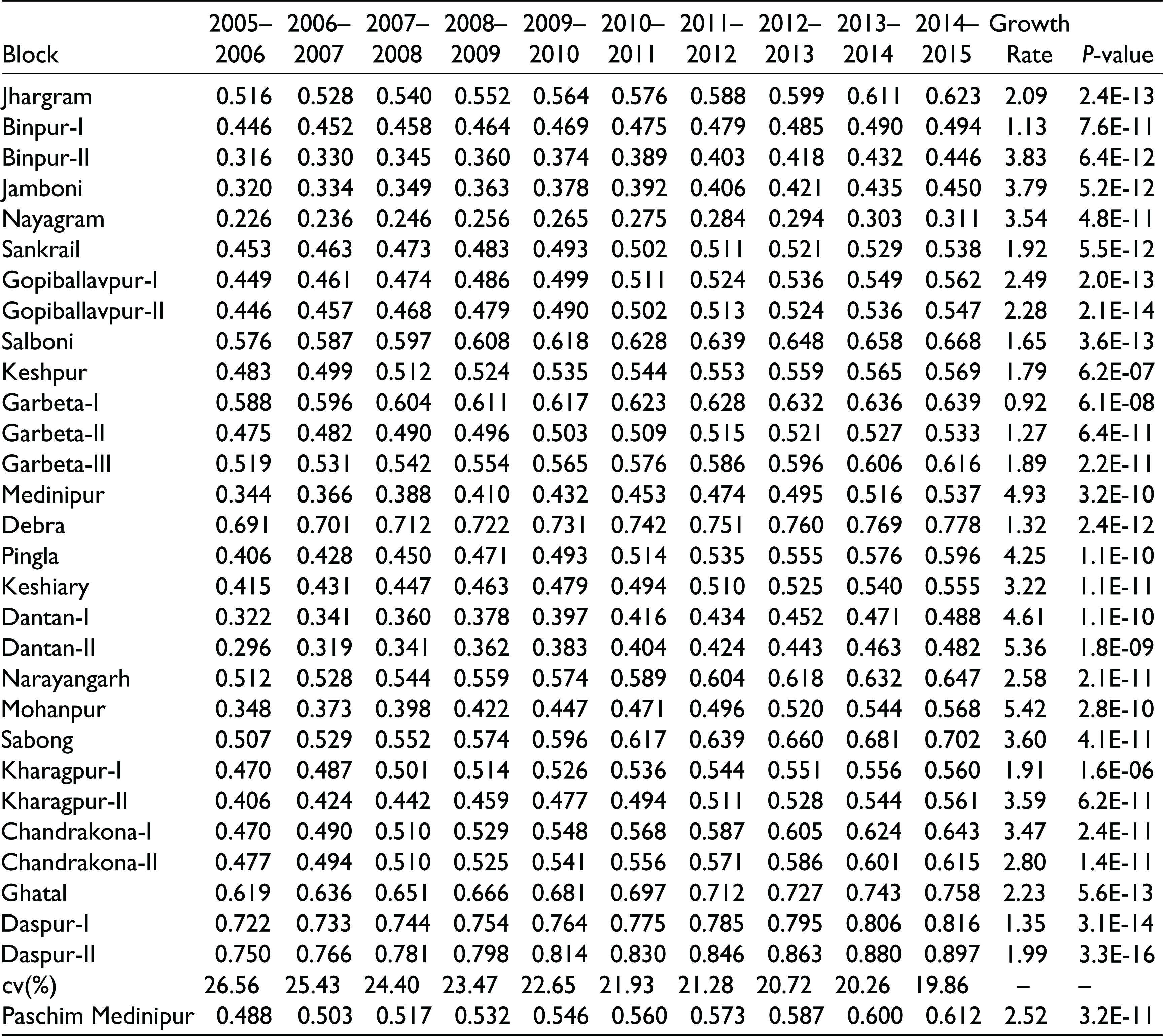
We have tried to make a complete assessment on the nature and variation of SL in 29 blocks of Paschim Medinipur district for the mentioned period of 2005–2006 to 2014–2015. The SLI is constructed on the basis of two dimensions, APLI and MWPRI, in which the respective weights of the dimensions are obtained by applying IACM as 65.29 per cent and 34.71 per cent and by using these weights respective SLIs for the blocks are calculated (refer to Table 1).

As noted by Anand and Sen (2000),

The income level enjoyed, especially close to poverty lines, can be very crucial information on the causal antecedents of basic human capabilities. The use of “command over resources” in the HDI is strictly as a residual catch-all, to reflect something of other basic capabilities not already incorporated in the measures of longevity and education.

In the absence of income or even expenditure data at block level, we have used APLI and MWPRI as the variables reflecting SL of which APLI is observed to have almost 2/3 weight and this reflects the judgement given by Anand and Sen above.

In this context, it can be mentioned that Health Index (HI) and Education Index (EI) are the covariates of SLI in the construction of Block Human Development Index (BHDI) and their weights are obtained as 45.72 per cent, 30.88 per cent and 23.41 per cent, respectively.

With reference to Table 1, it is observed that the growth rate of SLI is highest in Mohanpur (5.42) with level of significance at 2.8E-10, followed by Dantan-II (5.36) with level of significance at 1.8E-09 and Medinipur (4.93) with level of significance at 3.2E-10, whereas it is the lowest in Garbeta-I (0.92) with level of significance at 6.1E-08, followed by Binpur-I (1.13) with level of significance 7.6E-11 and Garbeta-II (1.27) with level of significance 6.4E-11. It is also observed that the blocks which had high SLI values at the initial stage, accrue lower growth rates (e.g., Daspur-I, Daspur-II, Keshpur, etc.) and the blocks with low SLI initially, achieved higher growth rates in SLI (e.g., Jamboni, Nayagram, Medinipur, etc.). It is to be noted that, inequality can be measured either by using Gini coefficients (gc) or by using the relative measure of the coefficient of variation (cv). To us, the “cv measure” of inequality is better accepted as it is value-based whereas the “gc measure” is purely rank based. We have tried to estimate the level of inequality prevailing across the said blocks during the study period and observed that it is diminishing over the years. As obtained from our work, for the year 2005–2006, “cv” is 26.56 per cent and it gradually moves to 19.86 per cent for the year 2014–2015 implying a reducing trend over the period of 10. Two dimension indices of SLI, namely APLI and MWPRI, for the blocks of Paschim Medinipur district for all the years are given in the Appendices.

Table 1.

Computation of SLI by Using IACM, for 29 Blocks of Paschim Medinipur District for the Period 2005–2006 to 2014–2015 and Their Respective Growth Rates and Levels of Significance

Block	2005–2006	2006–2007	2007–2008	2008–2009	2009–2010	2010–2011	2011–2012	2012–2013	2013–2014	2014–2015	Growth Rate	P-value
Jhargram	0.516	0.528	0.540	0.552	0.564	0.576	0.588	0.599	0.611	0.623	2.09	2.4E-13
Binpur-I	0.446	0.452	0.458	0.464	0.469	0.475	0.479	0.485	0.490	0.494	1.13	7.6E-11
Binpur-II	0.316	0.330	0.345	0.360	0.374	0.389	0.403	0.418	0.432	0.446	3.83	6.4E-12
Jamboni	0.320	0.334	0.349	0.363	0.378	0.392	0.406	0.421	0.435	0.450	3.79	5.2E-12
Nayagram	0.226	0.236	0.246	0.256	0.265	0.275	0.284	0.294	0.303	0.311	3.54	4.8E-11
Sankrail	0.453	0.463	0.473	0.483	0.493	0.502	0.511	0.521	0.529	0.538	1.92	5.5E-12
Gopiballavpur-I	0.449	0.461	0.474	0.486	0.499	0.511	0.524	0.536	0.549	0.562	2.49	2.0E-13
Gopiballavpur-II	0.446	0.457	0.468	0.479	0.490	0.502	0.513	0.524	0.536	0.547	2.28	2.1E-14
Salboni	0.576	0.587	0.597	0.608	0.618	0.628	0.639	0.648	0.658	0.668	1.65	3.6E-13
Keshpur	0.483	0.499	0.512	0.524	0.535	0.544	0.553	0.559	0.565	0.569	1.79	6.2E-07
Garbeta-I	0.588	0.596	0.604	0.611	0.617	0.623	0.628	0.632	0.636	0.639	0.92	6.1E-08
Garbeta-II	0.475	0.482	0.490	0.496	0.503	0.509	0.515	0.521	0.527	0.533	1.27	6.4E-11
Garbeta-III	0.519	0.531	0.542	0.554	0.565	0.576	0.586	0.596	0.606	0.616	1.89	2.2E-11
Medinipur	0.344	0.366	0.388	0.410	0.432	0.453	0.474	0.495	0.516	0.537	4.93	3.2E-10
Debra	0.691	0.701	0.712	0.722	0.731	0.742	0.751	0.760	0.769	0.778	1.32	2.4E-12
Pingla	0.406	0.428	0.450	0.471	0.493	0.514	0.535	0.555	0.576	0.596	4.25	1.1E-10
Keshiary	0.415	0.431	0.447	0.463	0.479	0.494	0.510	0.525	0.540	0.555	3.22	1.1E-11
Dantan-I	0.322	0.341	0.360	0.378	0.397	0.416	0.434	0.452	0.471	0.488	4.61	1.1E-10
Dantan-II	0.296	0.319	0.341	0.362	0.383	0.404	0.424	0.443	0.463	0.482	5.36	1.8E-09
Narayangarh	0.512	0.528	0.544	0.559	0.574	0.589	0.604	0.618	0.632	0.647	2.58	2.1E-11
Mohanpur	0.348	0.373	0.398	0.422	0.447	0.471	0.496	0.520	0.544	0.568	5.42	2.8E-10
Sabong	0.507	0.529	0.552	0.574	0.596	0.617	0.639	0.660	0.681	0.702	3.60	4.1E-11
Kharagpur-I	0.470	0.487	0.501	0.514	0.526	0.536	0.544	0.551	0.556	0.560	1.91	1.6E-06
Kharagpur-II	0.406	0.424	0.442	0.459	0.477	0.494	0.511	0.528	0.544	0.561	3.59	6.2E-11
Chandrakona-I	0.470	0.490	0.510	0.529	0.548	0.568	0.587	0.605	0.624	0.643	3.47	2.4E-11
Chandrakona-II	0.477	0.494	0.510	0.525	0.541	0.556	0.571	0.586	0.601	0.615	2.80	1.4E-11
Ghatal	0.619	0.636	0.651	0.666	0.681	0.697	0.712	0.727	0.743	0.758	2.23	5.6E-13
Daspur-I	0.722	0.733	0.744	0.754	0.764	0.775	0.785	0.795	0.806	0.816	1.35	3.1E-14
Daspur-II	0.750	0.766	0.781	0.798	0.814	0.830	0.846	0.863	0.880	0.897	1.99	3.3E-16
cv(%)	26.56	25.43	24.40	23.47	22.65	21.93	21.28	20.72	20.26	19.86	–	–
Paschim Medinipur	0.488	0.503	0.517	0.532	0.546	0.560	0.573	0.587	0.600	0.612	2.52	3.2E-11

Sources: (i) Registrar General of India (1991, 2001, 2011).

(ii) Government of West Bengal (various years).

Moreover, it is also observed that the blocks which have negative MWPRI such as Binpur-I, Nayagram and Garbeta-II are having positive SLI growth rate and this might be attributed to the fact that there exists a strong positive impact of APLI on SLI. On the contrary, the block of Kharagpur-I had a negative APLI (–0.16) even if it goes to achieve positive SLI, as its MWPRI was strong enough to counterbalance the negativity of APLI. The district of Paschim Medinipur, except the municipal areas, performed ordinarily in SLI in terms of growth rate (i.e., 2.52) and this is due to the fact that the initial value was not that poor. From the SLI analysis, it is also found that the rate of growth of SLI in most of the blocks are high and above the district average which indicates progress towards achievement of a better SL.

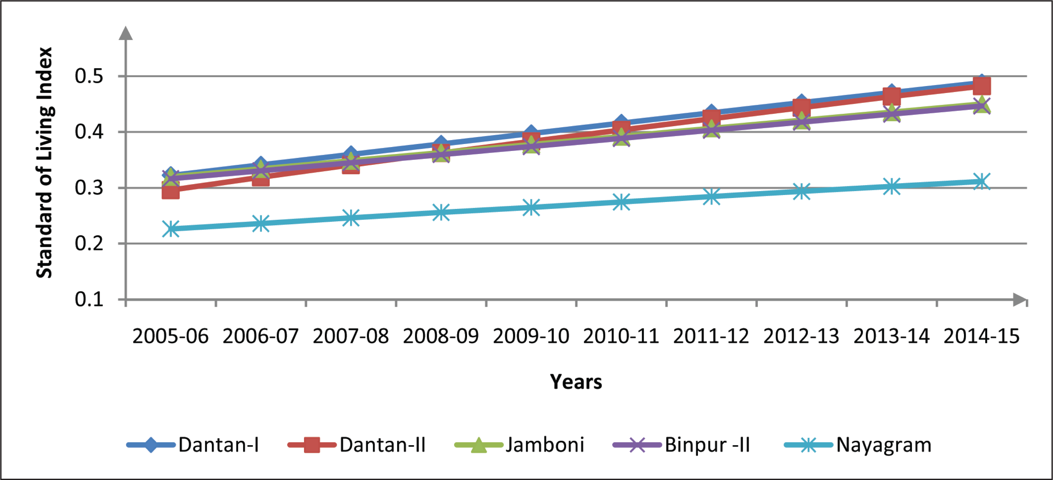
With reference to Figures 1 and 2, the trend lines of the best five performing blocks and the worst five performing blocks of Paschim Medinipur district in terms of SLI values (as found in the index values for 2014–2015) for the range period of 2005–2006 to 2014–2015 are shown. It is observed from Figure 1 that the trend lines for the best five blocks Daspur-II, Daspur-I, Debra, Ghatal and Sabong are upward rising straight lines, no one intersecting other, maintaining almost same slope all through, implying that these blocks are steadily progressing to achieve higher values over time. On the other hand, from Figure 2, it is observed that the five most poorly performing blocks are Dantan-I, Dantan-II, Jamboni, Binpur-II and Nayagram, but their trend lines are also upward-rising. However, the slopes are not, all the same, this time as we find that the slope of the trend line for Dantan-II is higher and those for Jamboni and Nayagram are relatively lower indicating variances in degree of progress in SLI.

Figure 1.

Source: Authors’ own calculation.

Figure 2.

Source: Authors’ own calculation.

Factor Analysis of Standard of Living in Pooled and Panel Data Frameworks

Factors Affecting Standard of Living

Living standard of a region as obtained by the values of SLI (calculated above) is supposed to depend upon a number of factors that represent the economic status of the concerned region which may be a block or a district or a state or a country. The factors may be enumerated as follows:

Demographic factor, measured through LTR: Demographic quality can be considered as an effective factor to attain better SL in any particular area. For this article, we have selected general LTR as a suitable parameter to catch the demographic quality of the area.

Employment Status of the people, measured through NAGL: Employment status of the people of a region can be understood by observing the job pattern prevailing in that area. In this article, we shall find out the ratio of non-agricultural labour to total available labour force and obtain the NAGL as a parameter of employment status.

Social status of the people, measured through Scheduled Tribe Ratio (STR): Historically, it is observed that STs are economically backward, mostly very poor, concentrated in low-skill occupations and primarily rural. According to the 2011 census, the STs are about 8.6 per cent in India’s population. The percentage shares of ST population in total population of the district of Paschim Medinipur are 14.87 in 2001 and 14.88 in 2011, which are far above the state average (5.50% in 2001 and 5.8% in 2011) of West Bengal. This motivates us to consider the ST population separately in this study. Here we do hypothesize a negative relationship between the ratio of ST people (STR) and attainment in SLI.

Urbanization of the area, measured through PD: Urbanization implies increase in percentage of population living in statutory towns, census towns, urban agglomerations and urban out-growths with a high PD. The process of urbanization is often linked with industrialization and moder-nization, as large numbers of people in the urban area are found to be engaged in non-farm activities. PD is included here as a proxy variable of urbanization with the hypothesis that it influences SLI directly.

Availability of food in the area, measured through Per Capita Food Grains Production (PCFGP): Food is considered as the basic need of an area and other developmental activities are to gain momentum, once adequate food supply is ensured. Here, we are considering PCFGP as the parameter to measure availability of food and hypothesize that PCFGP maintains a positive relationship with the SLI.

Empirical Methodology and Benchmark Results

Now we shall examine the impact of LTR, NAGL, Schedule Tribe Ratio (STR), PD and Per Capita Food Grain Production (PCFGP) on SLI for the blocks of Paschim Medinipur district in West Bengal, India for the period 2005–2006 to 2014–2015. We do consider ordinary least squares (OLS) specifications and try to estimate the simple, partial, ortho-partial and relative importance of different determining factors of SLI.

Thus, our empirical specification is as follows: Y₁X₁₂X₂₃X₃₄X₄₅X₅_i

Where, Y stands for the SLI, X₁ is LTR, X₂ is NAGL, X₃ is STR, X₄ is PD and X₅ is PCFGP, α is the intercept parameter and Ɛ_i is the disturbance term. The coefficient of X_j, denoted by β_j, measures the amount of change in Y for one unit change in X_j, the values of all other explanatory variables remaining constant; the coefficient is thus known as the partial regression coefficient.

Results of Pooled Data Analysis

Table 2 shows the results of pooled regression of Y (SLI) on X₁ (LTR)_, X₂ (NAGL)_, X₃ (STR)_, X₄ (PD) and X₅ (PCFGP). We observe that the coefficient of determination, that is, R² is 0.4987, which is statistically significant (level of significance 1.18E-40). Here coefficients of all five factors, namely LTR, NAGL, PD, WPR and PCFGP are statistically significant as are found from their t-values and p-values obtained from multiple regression. LTR, NAGL, PD and PCFGP are directly related to SLI and STR is inversely related to SLI.

Table 2.

Results from Pooled Regression of SLI on Its Determinants

Variable	Coef.	T-value	P-value	Sq. Partial Correlation	Coef.	T-value	P-value	Sq. Simple Correlation
LTR	0.00323	2.78	5.80E-03	0.0265	0.01066	11.97	4.37E-27	0.3324
NAGL	0.00526	2.87	4.41E-03	0.0282	0.01648	13.12	3.91E-31	0.3740
STR	–0.00138	–1.66	9.71E-02	0.0097	–0.00678	–12.19	7.91E-28	0.3402
PD	0.00014	3.87	1.37E-04	0.0500	0.00029	14.21	4.18E-35	0.4123
PCFGP	0.00002	1.85	6.47E-02	0.0120	0.00003	1.61	1.08E-01	0.0090
R ²	Adj R²	F-Value	P-Value
0.4987	0.4899	57	1.18E-40
Variable	Coef.	T-value	P-value	Sq. Ortho-partial Correlation		Variable	Relative Importance	T-value of Relative Importance
LTR	0.00323	2.00	4.69E-02	0.0136		LTR	0.1086	5.92
NAGL	0.00526	2.06	4.02E-02	0.0145		NAGL	0.1250	6.42
STR	–0.00138	–1.19	2.35E-01	0.0049		STR	0.1082	–5.91
PD	0.00014	2.79	5.55E-03	0.0264		PD	0.1496	7.12
PCFGP	0.00002	1.33	1.86E-01	0.0061		PCFGP	0.0073	1.45

Source: Authors’ own calculation.

Note: Bold values indicate ortho-partial correlation and relative importance.

These t-values indicate squared correlations of the factors with SLI (r² = t² / (t² + degree of freedom)) and in the existing literature, they are known as partial correlation of the factors. Here we observe that PD is the most significant factor which explains partially 5.00 per cent of the variability of Y followed by NAGL which explains about 2.82 per cent of the variability of Y. LTR is the third significant variable which explains about 2.65 per cent of the variability of Y. PCFGP is the fourth significant variable which explains about 1.20 per cent of the variability of Y. STR is the least significant variable and it explains only about less than 0.97 per cent of the variability of Y. However, these are not true partial correlations as explained by Mondal (2008). For example, the partial correlation of PD is 0.05 which implies that that part of PD which is not linearly explained by other 4 factors is able to explain 5 per cent of the variability of that part of SLI which is not linearly explained by those other 4 factors. Here, other 4 factors explain 47.23 per cent of the variability of SLI. Therefore, that part of PD which is not linearly explained by other 4 factors is able to explain 2.64 per cent (49.87% – 47.23%) of the variability of SLI which is 5 per cent of 52.77 per cent (= 100% – 47.23%), the part of SLI which is not linearly explained by other 4 factors. Thus, PD is partially explaining 2.64 per cent of the variability of SLI or 5 per cent of the variability of that part of SLI which is not linearly explained by other 4 factors and this 2.64 per cent is its true partial correlation named as ortho-partial correlation by Mondal (2008). Thus, partial correlation (henceforth, we shall call it pseudo partial correlation) of any variable actually overestimates true partial correlation or ortho-partial correlation of the variable. Ortho-partial correlations of other 4 factors, that is, X_1, X_2, X₃ and X₅ are 0.0136, 0.0145, 0.0049 and 0.0061, respectively (these are actually values of r² (a) in the regression of Y on the residue of X₁ obtained from the regression of X₁ on X_2, X₃, X₄ and X₅; (b) in the regression of Y on the residue of X₂ obtained from the regression of X₂ on X₁, X₃, X₄ and X₅; (c) in the regression of Y on the residue of X₃ obtained from the regression of X₃ on X₁, X₂, X₄ and X₅ and (d) in the regression of Y on the residue of X₅ obtained from the regression of X₅ on X₁, X₂, X₃ and X₄, respectively).

Ortho-partial correlations differ from their respective simple correlation due to overlapping nature among the variables or due to multi-collinearity. In our case, we observe that for variables X₁ (LTR), X₂ (NAGL), X₃ (STR), X₄ (PD) and X₅ (PCFGP), simple correlations are greater than ortho-partial correlations. This is due to multi-collinearity with no enhancement-synergism or due to positive overlapping. For all five variables, ortho-partial correlations underestimate whereas simple correlations overestimate the relative importance of the variables. Thus, neither the simple correlations nor the ortho-partial correlations can properly estimate the relative importance of the explanatory factors. Partial correlations are always greater than ortho-partial correlations, so they overestimate the true partial correlations and may either underestimate or truly estimate or overestimate the relative importance of the explanatory factors. Several attempts are made in the literature to evaluate relative importance of the explanatory factors. We, in reference to one such attempt, shall try to evaluate the relative importance of explanatory factors explaining the variability of SLI.

True relative importance of an explanatory variable can be obtained by averaging squared simple correlation and squared ortho-partial correlation in case of two explanatory variables and by averaging squared simple correlation, a series of squared semi ortho-partial correlations and squared ortho-partial correlation in case of more than 2 explanatory variables. Here we observe that the squared simple correlations of LTR (X₁), NAGL (X₂), STR (X₃), PD (X₄) and PCFGP (X₅) with SLI (Y) are respectively r₁² = 0.3324, r₂² = 0.3740, r₃² = 0.3402, r₄² = 0.4123 and r₅² = 0.0090. LTR, NAGL, STR and PD are statistically highly significant but PCFGP is not statistically significant. Squared ortho-partial correlations of LTR, NAGL, STR, PD and PCFGP with SLI (Y) are respectively 0.0136, 0.0145, 0.0049, 0.0264 and 0.0061. LTR, NAGL, PD and PGR are statistically significant but STR and PCFGP are not.

It is observed that for PCFGP, the respective simple correlation and ortho-partial correlation values are very low and statistically not significant. But as the pseudo partial correlation value of this variable is statistically significant or as this variable is able to explain a significant part of the variability of that part of SLI which is not linearly explained by other four factors, we do not exclude the variable from the model. Here we see that the t-values of LTR, NAGL, PD and PCFGP are positive (+ve) in simple, partial and ortho-partial regressions and those for STR is negative. Enhancement-synergism is mildly present at some semi ortho-partial level.

As we have already said, the relative importance of an explanatory variable lies between the squared ortho-partial correlation and the squared simple correlation, the relative importance of the variable can be calculated by averaging these two through a series of squared semi ortho-partial correlations. For example, for the first variable, that is, LTR has the squared ortho-partial correlation of 0.0136 which is less than squared simple correlation of 0.3324; the relative importance of the variable is calculated to be 0.1086 with a significant negative t-value.

In fact, relative importance is considered as the real contribution of a particular factor in explaining the dependent variable (i.e., the final index). There might be some sort of overlapping in the values of simple correlation, whereas ortho-partial correlation indicates typical segmented non-overlapping value of a factor, leaving aside the conjoint areas of explanation. Hence, the average of all three forms of correlation (i.e., the simple, the ortho-partial and the semi ortho-partial, if any) is needed for a particular factor to establish its relative importance amongst all in explaining the dependent variable.

In this way, relative importance of other 4 explanatory variables, that is, NAGL, STR, PD and PCFGP, are calculated at 0.1250, 0.1082, 0.1496 and 0.0073 respectively. Thus the multiple R² of 0.4987 that implies an explanatory power of 49.87 per cent is decomposed among the explanatory factors in the following way: 10.86 per cent of the variability of SLI is explained by LTR, 12.50 per cent by NAGL, 10.82 per cent by STR, 14.96 per cent by PD and 0.73 per cent by PCFGP and except PCFGP all of them have t-values statistically significant at less than 1 per cent level of significance. In this connection, it can be noted that partial correlations underestimate relative importance of the first four variables, that is, LTR, NAGL, STR and PD, and overestimate relative importance of the last variable, that is, PCFGP.

Even if pooled data analysis is providing a satisfactory explanation regarding the behaviour of the determining factors of SL in our context, besides this, we are also interested in knowing the inter-temporal (i.e., within group) and inter-block (i.e., between groups) variations in SLI which have occurred due to the chosen factors of SL. As we are enriched with both time series and cross-section observations on the variables in our study, we can use the panel data framework to undergo the same and obtain some results.

Results of Panel Data Analysis

In this section, we have analysed the prominence of the five factors in terms of short panel regressions. We suppress panel data regression to explain the role of different factors in explaining within-group (inter-temporal), between-group (inter-block) variation and also overall variation in SLI for all concerned periods taken together. Panel data regressions are very useful in the sense that it encompasses both the time series and cross-section data and its underlying heterogeneity helps significantly to understand the nature of the influential factors. This type of regression analysis further simplifies computation and inference, gives more informative data, more sample variability, evaluates the effectiveness, proposes micro foundations for aggregate data analysis, shows less co-linearity among variables, greater capacity for capturing complexity and more efficiency which can profusely detect and measure effects that are not found effectively in pure cross-section or pure time series data. The regression model of panel data can be estimated by three fashionable and convenience techniques, namely the REM, the FEM and the pooled regression model (OLS). We cannot arbitrarily choose any one technique from these three for estimation. For selecting the best-fitted model, we have used two very popular tests, namely the Breusch–Pagan LM test for random effect and the Hausman specification test, in which Breusch–Pagan LM test estimates whether the REM is better fitted than the pooled regression model or not. If there is a significant χ²-value of Breusch–Pagan LM test or the P-value of χ² is less than a specified level of significance then REM is better fitted than pooled regression model. Hausman specification test also estimates whether FEM is better fitted than REM or not. If there is a significant χ²-value of Hausman specification test or the P-value of χ² is less than a specified level of significance, it indicates that there is no systematic difference in coefficients which portfolios that FEM is better fitted than REM.

In Table 3, we present panel data results from the regression of SLI on the five variables separately. All these regressions are run under FEM. From Table 3, individual importance and individual significance of the factors which are affecting SLI are observed. Here we observe that PD has highest overall explanatory power (overall R² = 0.4123) followed by NAGL (overall R² = 0.3740) and STR (overall R² = 0.3402). PCFGP has lowest overall R² (0.0090) preceded by LTR (0.3324).

Table 3.

Results from Separate Panel Regressions of SLI on Its Determinants

SLI	Coefficient	S. E.	T-value	P > \|t\|	Within R²	Between R²	Overall R²
LTR	0.00650	0.00051	12.69	0.0000	0.3826	0.3570	0.3324
NAGL	0.01280	0.00099	12.92	0.0000	0.3909	0.3770	0.3740
STR	–0.03268	0.00377	–8.67	0.0000	0.2245	0.3732	0.3402
PD	0.00134	0.00005	29.15	0.0000	0.7657	0.4275	0.4123
PCFGP	0.00002	0.00001	2.77	0.0060	0.0287	0.0069	0.0090

Source: Authors’ own calculation.

Here we also observe that PD is the most significant factor (t-value is 29.15), the second significant factor is NAGL (t-value is 12.92) and the third significant factor is LTR (t-value is 12.69) followed by STR and PCFGP.

When all five variables are considered in panel regression, it is customary to run both the FEM and the REM to test whether they are giving significant fit or not to test whether they are giving better fit than OLS or not and if all these are satisfied then to test whether FEM is significantly giving a better fit than REM or not. The last test is performed by the Hausman specification test for model selection.

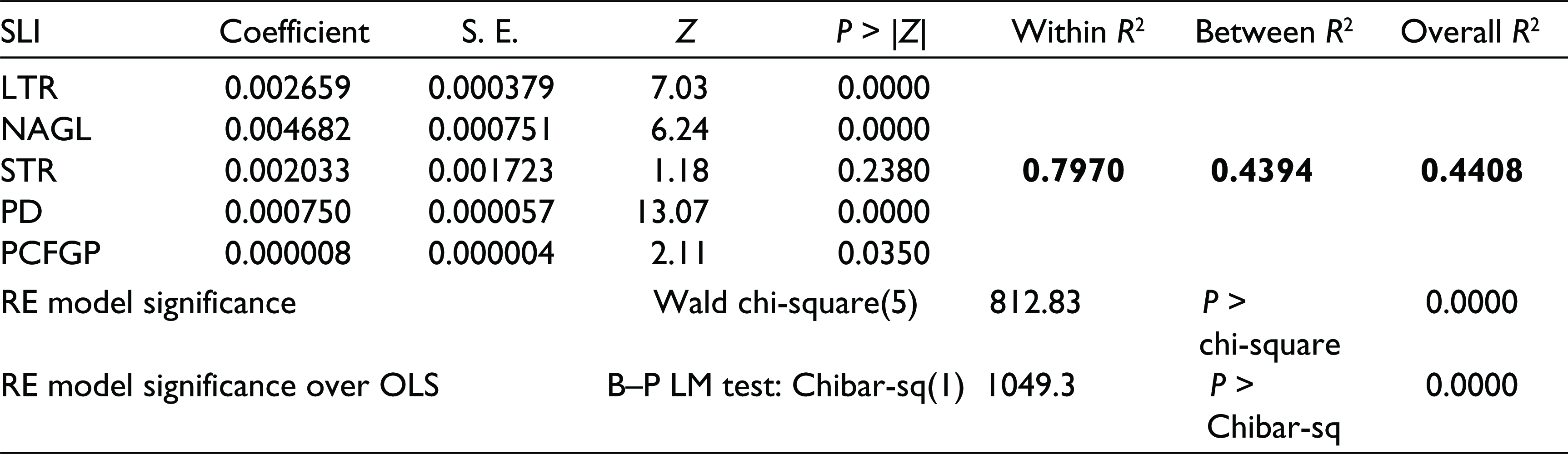
Results for both REM and FEM are presented in Tables 4 and 5 respectively for five explanatory variables (LTR, NAGL, STR, PD and PCFGP). Table 4 represents that the REM is itself a significant model for explaining variability of SLI (P-value of χ2 is close to 0) and REM carries higher significance over OLS because its P-value of χ2 is also close to 0. We also observe that the overall R² is low (44.08) in comparison to FEM and the factor of STR is insignificant, even if it has a positive relationship with SLI.

Table 4.

Results from Panel Regression of SLI on LTR, NAGL, STR, PD and PCFGP for the Blocks During the Period 2005–2006 to 2014–2015 (Random Effect Model)

SLI	Coefficient	S. E.	Z	P > \|Z\|	Within R²	Between R²	Overall R²
LTR	0.002659	0.000379	7.03	0.0000
NAGL	0.004682	0.000751	6.24	0.0000
STR	0.002033	0.001723	1.18	0.2380	0.7970	0.4394	0.4408
PD	0.000750	0.000057	13.07	0.0000
PCFGP	0.000008	0.000004	2.11	0.0350
RE model significance			Wald chi-square(5)		812.83	P > chi-square	0.0000
RE model significance over OLS			B–P LM test: Chibar-sq(1)		1049.3	P > Chibar-sq	0.0000

Source: Authors’ own calculation.

Note: Bold values indicate ortho-partial correlation and relative importance.

From Table 4 it is observed that FEM is itself a significant model for explaining the variability of SLI (P-value of the F-statistic is close to 0), and FEM carries higher significance over OLS because the P-value of the corresponding F-statistic is also close to 0. This indicates that FEM is better fitted than OLS. Finally, from the Hausman specification test, it is found that there is a systematic difference in coefficients which is statistically significant and so the FEM turns out to be better fitted than the REM. Hence, we analyse the results of short panel regression under FEM of Table 5.

Table 5.

Results from Panel Regression of SLI on LTR, NAGL, STR, PD and PCFGP for the Blocks During the Period 2005–2006 to 2014–2015 (Fixed Effect Model)

SLI	Coefficient	S. E.	T	P > \|t\|	Within R²	Between R²	Overall R²
LTR	0.00200	0.000328	6.08	0.0000
NAGL	0.00307	0.000658	4.66	0.0000
STR	–0.00673	0.002009	–3.35	0.0010	0.8265	0.4566	0.4436
PD	0.00098	0.000055	17.82	0.0000
PCFGP	0.00001	0.000003	1.65	0.1000
FE model significance				F(5,256)	243.83	P > F	0.0000
FE model significance over OLS				F(28, 256)	223.36	P > F	0.0000
RE-FE model comparison			Hausman: chi-square(5)		55.72	P > chi-square	0.0000

Source: Authors’ own calculation.

Note: Bold values indicate ortho-partial correlation and relative importance.

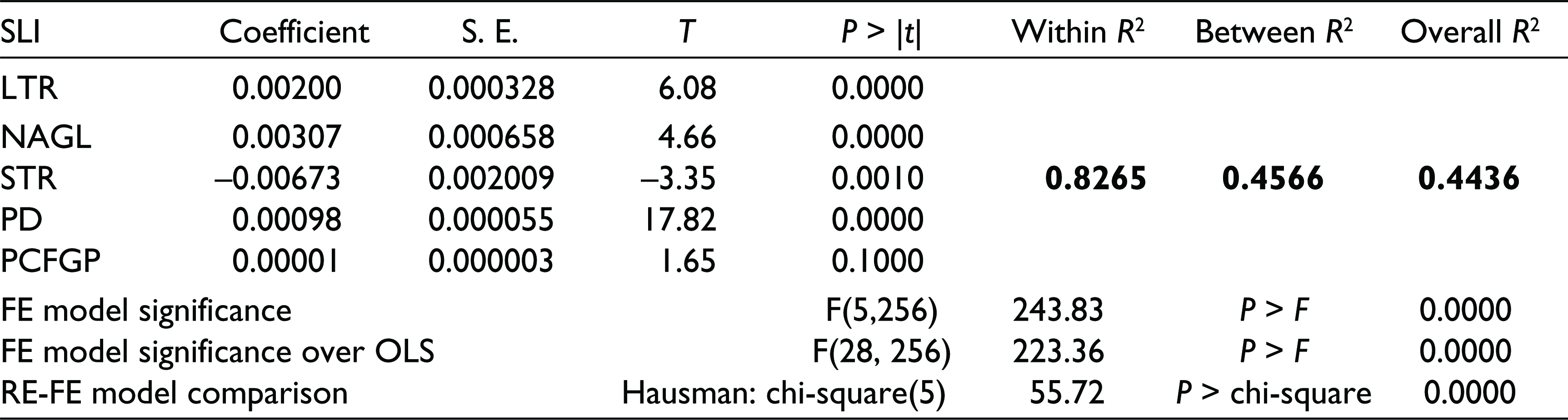
From Table 5, we observe that the overall explanatory power (R²) of the above mentioned 5 factors taken together is 44.36 per cent, within a group (here within-block and basically inter-temporal) explanatory power (R²) is 82.65 per cent and between groups (here between blocks) explanatory power is 45.66 per cent. It is observed that PD is partially the most significant factor (t-value is 17.82) in explaining the variability of SLI followed by LTR with t-value at 6.08. The third partially significant factor is NAGL (t-value is 4.66) followed by STR (t-value is –3.35) and PCFGP (t-value is 1.65). PD, LTR, NAGL and STR are statistically significant at less than 1 per cent level of significance but PCFGP is statistically significant at less than 10 per cent level of significance. It is also observed that SLI is positively associated with LTR, NAGL, PD and PCFGP, whereas it is negatively associated with STR.

In both pooled and panel data analysis, nearly 44 per cent (overall R² is 0.4436) to 50 per cent (multiple R² is 0.4987) of total variation (inter-temporal variation and between blocks variation) of SLI is explained by the five factors, namely LTR, NAGL, STR, PD and PCFGP. In both models, SLI is positively associated with LTR, NAGL, PD and PCFGP whereas it is negatively associated with STR. All the factors are found to be statistically significant as revealed by the t-statistic. It goes beyond saying that increased literacy accounts for high demographic quality and this, in turn, is supposed to lead towards better employment opportunities, better earning in a sustainable manner and thereby higher SL. Thus the positive relation between LTR and SLI, as obtained in our empirical test, is justified. Second, higher work participation in non-agricultural sector of any locality is bound to increase the relative earning capacity of the households as well as the status of the households and thereby enhances their attitude towards better living. Hence, the positive relationship between NAGL and SLI is conceived in this analysis. Third, the positive association between SLI and PD (i.e., PD), as we have found, might be due to high PD in the census towns of the blocks because of high concentration of economic activities and business transactions in the blocks, leading to better SL. Fourth, the factor of food supply is measured through PCFGP and this analysis has established a positive relation of it with the SLI. It is obvious that, if adequate food supply is ensured in a place, people of that area would be motivated more to take high-level skills and training to find better job placement. This may lead to better living facilities to the households of that area in a sustainable manner and this is what we have obtained through our study. Finally, we have found that there exists a negative relationship between the STR and the SLI in our study. It is a historical fact that, in India, the ST people are generally less educated and are primarily engaged in agricultural sector; and those people are not in a position to think or visualize about a better or higher way of living. Our study area is no exception. Hence we can argue that, if there prevail a significant portion of ST people in the area, there is a possibility that the SLI of that area might be low.

Concluding Remarks

The concept of SL in social sciences is the appetite of an individual or group for foods and services. In other words, SL is the assessment of goods and services produced and available to purchase by a person, family, group or nation. A SL is the level of wealth, comfort, material goods and necessities available to a certain socio-economic class or a certain geographic area. It includes factors such as income, gross domestic products, national income growth, economic and political stability, political and religious freedom, environmental quality, climate and safety. It is closely related to quality of life.

Determining a country’s SL is really a complex art rather than an exact science because there are elements of it that are hard to quantify. For example, it is often presumed that living in a country with a democratic political system and a free press improves the SL, but this is not exactly easy to reduce it to numbers. Consequently, economists typically try to simplify the measure by using only economic factors that are subject to measurement and mathematical calculation.

In this study, we have successfully computed an appropriate composite SLI by using IACM on the basis of all important indicators for attainment of living standard for the blocks of Paschim Medinipur district in West Bengal over the period of 2005–2006 to 2014–2015. Among the blocks, Daspur-II, Daspur-I, Ghatal, Sabong, Debra are the overall top performers and Nayagram, Binpur-II, Jamboni, Dantan-II and Gopiballavpur-I are bottom-level performers in attainment of living standard. Our study reveals that most of the blocks of Paschim Medinipur district have achieved improvement in respect to attainment in SL over time. It is also seen that both inter-block variation and inter-temporal variation of SLI are significant though inter-block variation is more significant than inter-temporal variation. This both way variations of SLI is observed to be significantly explained by various socio-economic and demographic factors such as LTR, NAGL, STR, PD and PCFGP. We have also tried to calculate the pseudo partial importance (through squared partial correlation), true or correct partial importance (through squared ortho-partial correlation) and relative importance (through squared average correlation) of the explanatory factors by using the pooled regression framework and the pseudo partial importance (through partial correlation) of the explanatory factors by using the panel regression framework. From the pooled regression results, it appears that the PD is the most important factor with relative importance of 0.1496 out of 0.4987. This factor is observed to affect the SLI positively and its possible justification is briefed in the last part of the section “Factor Analysis of Standard of Living in Pooled and Panel Data Frameworks.” It is also revealed from the pooled regression that NAGL is the second important factor with relative importance of 0.1250 out of 0.4987. This factor is also observed to affect SLI positively. The policy implication of this finding is that efforts should be made to extend socio-economic facilities (i.e., amenities) which are generally found in urban areas, in the rural areas of the district also, to improve the SLI of the area concerned. A similar discussion is found in Pattanayek and Mondal (2016) in case of Education Index in the blocks of Paschim Medinipur district.

From the analysis of Panel regression, we observe that the above mentioned five factors are significant in explaining the variability of SLI. The signs of the coefficients of these factors are same as those which are obtained through pooled regression. From the significance of the individual coefficients, nothing can be said about their relative importance because the significance here is based on pseudo partial correlations. What we can say is that they are jointly significant in explaining both the across-block and within-block variation in SLI. Thus, the policy implications mentioned above in the context of pooled regression may also apply in the context of panel regression. Finally, it can be said that the list of selected factors that are affecting SLI is not exhaustive. The future researchers, working in this area can take up the issue in a broad spectrum and carry on with better implications.

Footnotes

Appendix

Table A2.

Computation of MWPRI for 29 Blocks of Paschim Medinipur District for the Period 2005–2006 to 2014–2015 and Their Respective Growth Rates and Levels of Significance

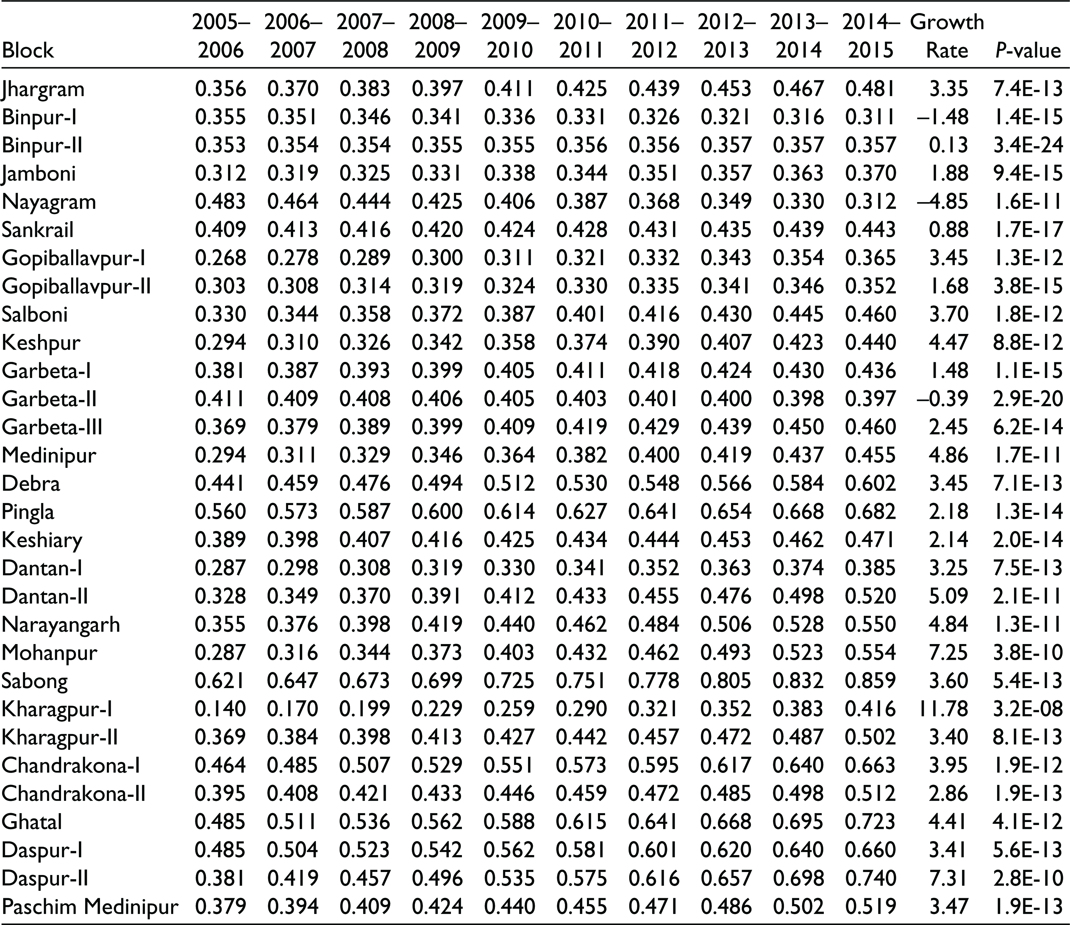
Block	2005– 2006	2006– 2007	2007– 2008	2008– 2009	2009– 2010	2010– 2011	2011– 2012	2012– 2013	2013– 2014	2014– 2015	Growth Rate	P-value
Jhargram	0.356	0.370	0.383	0.397	0.411	0.425	0.439	0.453	0.467	0.481	3.35	7.4E-13
Binpur-I	0.355	0.351	0.346	0.341	0.336	0.331	0.326	0.321	0.316	0.311	–1.48	1.4E-15
Binpur-II	0.353	0.354	0.354	0.355	0.355	0.356	0.356	0.357	0.357	0.357	0.13	3.4E-24
Jamboni	0.312	0.319	0.325	0.331	0.338	0.344	0.351	0.357	0.363	0.370	1.88	9.4E-15
Nayagram	0.483	0.464	0.444	0.425	0.406	0.387	0.368	0.349	0.330	0.312	–4.85	1.6E-11
Sankrail	0.409	0.413	0.416	0.420	0.424	0.428	0.431	0.435	0.439	0.443	0.88	1.7E-17
Gopiballavpur-I	0.268	0.278	0.289	0.300	0.311	0.321	0.332	0.343	0.354	0.365	3.45	1.3E-12
Gopiballavpur-II	0.303	0.308	0.314	0.319	0.324	0.330	0.335	0.341	0.346	0.352	1.68	3.8E-15
Salboni	0.330	0.344	0.358	0.372	0.387	0.401	0.416	0.430	0.445	0.460	3.70	1.8E-12
Keshpur	0.294	0.310	0.326	0.342	0.358	0.374	0.390	0.407	0.423	0.440	4.47	8.8E-12
Garbeta-I	0.381	0.387	0.393	0.399	0.405	0.411	0.418	0.424	0.430	0.436	1.48	1.1E-15
Garbeta-II	0.411	0.409	0.408	0.406	0.405	0.403	0.401	0.400	0.398	0.397	–0.39	2.9E-20
Garbeta-III	0.369	0.379	0.389	0.399	0.409	0.419	0.429	0.439	0.450	0.460	2.45	6.2E-14
Medinipur	0.294	0.311	0.329	0.346	0.364	0.382	0.400	0.419	0.437	0.455	4.86	1.7E-11
Debra	0.441	0.459	0.476	0.494	0.512	0.530	0.548	0.566	0.584	0.602	3.45	7.1E-13
Pingla	0.560	0.573	0.587	0.600	0.614	0.627	0.641	0.654	0.668	0.682	2.18	1.3E-14
Keshiary	0.389	0.398	0.407	0.416	0.425	0.434	0.444	0.453	0.462	0.471	2.14	2.0E-14
Dantan-I	0.287	0.298	0.308	0.319	0.330	0.341	0.352	0.363	0.374	0.385	3.25	7.5E-13
Dantan-II	0.328	0.349	0.370	0.391	0.412	0.433	0.455	0.476	0.498	0.520	5.09	2.1E-11
Narayangarh	0.355	0.376	0.398	0.419	0.440	0.462	0.484	0.506	0.528	0.550	4.84	1.3E-11
Mohanpur	0.287	0.316	0.344	0.373	0.403	0.432	0.462	0.493	0.523	0.554	7.25	3.8E-10
Sabong	0.621	0.647	0.673	0.699	0.725	0.751	0.778	0.805	0.832	0.859	3.60	5.4E-13
Kharagpur-I	0.140	0.170	0.199	0.229	0.259	0.290	0.321	0.352	0.383	0.416	11.78	3.2E-08
Kharagpur-II	0.369	0.384	0.398	0.413	0.427	0.442	0.457	0.472	0.487	0.502	3.40	8.1E-13
Chandrakona-I	0.464	0.485	0.507	0.529	0.551	0.573	0.595	0.617	0.640	0.663	3.95	1.9E-12
Chandrakona-II	0.395	0.408	0.421	0.433	0.446	0.459	0.472	0.485	0.498	0.512	2.86	1.9E-13
Ghatal	0.485	0.511	0.536	0.562	0.588	0.615	0.641	0.668	0.695	0.723	4.41	4.1E-12
Daspur-I	0.485	0.504	0.523	0.542	0.562	0.581	0.601	0.620	0.640	0.660	3.41	5.6E-13
Daspur-II	0.381	0.419	0.457	0.496	0.535	0.575	0.616	0.657	0.698	0.740	7.31	2.8E-10
Paschim Medinipur	0.379	0.394	0.409	0.424	0.440	0.455	0.471	0.486	0.502	0.519	3.47	1.9E-13

Source: (i) Registrar General of India (1991, 2001, 2011).

(ii) Government of West Bengal (various years).

Declaration of Conflicting Interests

The authors declared no potential conflicts of interest with respect to the research, authorship and/or publication of this article.

Funding

The authors received no financial support for the research, authorship and/or publication of this article.

References

Anand

, & Sen

(1994). Human Development Index: Methodology and measurement (Occasional Paper No. 12). New York, NY: Human Development Report Office, UNDP (Reprinted in Fukuda-Parr

& Shiv Kumar

A. K.

(Eds.), Readings in Human Development (2003). Oxford: Oxford University Press).

Anand

, & Sen

(2000). The income component of the Human Development Index. Journal of Human Development, 1(1), 83–106.

Blackorby

, & Russell

R. R.

(1978). Indices and sub-indices of the cost of living and the standard of living. Wiley for the Economics Department of the University of Pennsylvania and Institute of Social & Economic Research, 19(1), 229–240.

Deutsch

, & Silber

(1999). Religion, standard of living and the quality of life. Contemporary Jewry (Springer), 20(1), 119–137.

Government of India (2001). National Human Development Report of India. New Delhi: Planning Commission.

Government of India (2011). India Human Development Report 2011: Towards Social Inclusion. Institute of Applied Manpower Research, Planning Commission.

Government of West Bengal (2004). West Bengal Human Development Report, Development and Planning Department.

Government of West Bengal (2005). Rural Household Survey, Department of Panchayats and Rural Development.

Government of West Bengal (2010). Rural Household Survey, Department of Panchayats and Rural Development.

10.

Government of West Bengal. (2005–2015). District Statistical Handbook: Paschim Medinipur, Bureau of Applied Economic Research, Department of Planning and Statistics.

11.

Kumar

A. K. S.

(1991). UNDP’s Human Development Index: A computation for Indian states. Economic and Political Weekly, 26(41), 2343–2345.

12.

Kumar

A. K. S.

(1996). UNDP’s gender-related development index: A computation for Indian states. Economic & Political Weekly, 31(14), 887–895.

13.

Mondal

(2005). Human Development Index—An essay on methodology and implication. Kolkata: FIRMA KLM Private Limited.

14.

Mondal

(2008). On the test of significance of linear multiple regression coefficients. Communication in Statistics—Simulation and Computation, 37(4), 713–730.

15.

Mondal

, Mookherjee

, & Pattanayek

S. K.

(2017). Does the analysis of principal components effectively help in determining actual weights for dimensions of an index? An appraisal in Indian context. International Journal of Management and Development Studies, 6(10), 28–36.

16.

Morris

M. D.

(1980). The physical quality of life index (PQLI). Development Digest, 18(1), 95–109.

17.

Pattanayek

S. K.

, & Mondal

(2016). Educational development in blocks of Paschim Medinipur district (West Bengal) between 2005–2006 and 2012–2013: Panel data analysis through Education Index. Artha Vijnana, 58(1), 71–93.

18.

Registrar General of India (1991). Primary Census Abstract (PCA) of 1991. India Census 1991 (District-Level). New Delhi: Office of the Registrar General.

19.

Registrar General of India (2001). Primary Census Abstract (PCA) of 2001. India Census 2001 (District-Level). New Delhi: Office of the Registrar General.

20.

Registrar General of India (2011). Primary Census Abstract (PCA) of 2011. India Census 2011 (District-Level). New Delhi: Office of the Registrar General.

21.

Scholliers

(1996). Real wages and the standard of living in the nineteenth and early-twentieth centuries some theoretical and methodological elucidations. Franz Steiner Verlag, 83(3), 307–333.

22.

United Nations Development Programme (UNDP) (1990–2016). Human Development Report (HDR). New York, NY: Oxford University Press.