Abstract
A frequent empirical approach toward examining the impact of health on economic growth has been to focus on data for a cross-section of countries and to regress the income indicator on the health indicator controlling for the initial level of income and for other factors believed to influence steady-state income levels. From the methodological perspective, such a growth regression approach has mainly offered evidence for the relationship between health and income, using cross-country macro-level data. This article contributes to existing empirical research by introducing within-country regional-level analysis using three rounds of the Demographic and Health Surveys of Bangladesh, combined with corresponding geo-referenced global positioning system (GPS) data, to estimate the contribution of life expectancy to economic well-being. The joint evolution of the regional-level longevity and wealth indicator obtained from the micro-data corroborates Preston’s cross-country macro-level findings. Also, the finding that a 1 per cent increase in life expectancy leads to about 3 per cent increase in the wealth index corroborates the findings of several macro-regression studies and promotes the concept of direct investments in health.
1. INTRODUCTION
Investigation of the contribution of health to economic well-being is a well-trodden research area and until recently the literature, in general, has found evidence of a positive, significant and sizable influence of life expectancy (or some related health indicator) on economic growth. 1 This view, however, has been challenged by Acemoglu and Johnson (2007) who find there is no evidence that a large exogenous increase in life expectancy led to a significant increase in per capita economic growth. From the methodological perspective the growth regression approach has mainly offered evidence for the relationship between health and income using cross-country macro-level data. This article applies the growth regression method to examine, at the within-country geographic-regions level, the impact that health improvements may have had on economic well-being. For this purpose, the three rounds of survey data from the Demographic and Health Survey (DHS) of Bangladesh, combined with corresponding geo-referenced GPS data, are used.
2. THEORETICAL AND ESTIMATION FRAMEWORK
In order to show the impact of increased life expectancy on economic well-being, this article adopts the theoretical and estimation framework from Acemoglu and Johnson (2007), where a neo-classical Solow-type model is used. However, here the cross-country set-up in Acemoglu and Johnson (2007) has been replaced by the meso-level set-up, which is constituted of many geographic regions within the same country. The aggregate production function for the regions g within a country with constant returns to scale is given as:

where

Equation (2) shows that income per capita is affected positively by technology Ag, human capital, hg and the investment rate sg. Population, Ng, has a negative effect on income per capita. The impact of increased life expectancy enters into the model via three channels: increased population, increased human capital accumulation and a direct positive effect on total factor productivity. In the within-country regional context, these effects are captured by the following isoelastic functions:


where Xgt is the life expectancy in region g at time t;

where
The empirical approach to test the model parameters that capture the impact of the health variable on economic well-being is to estimate Equation (5). This article uses panel data where the units of observations are the region and time (three rounds of surveys conducted in 2000, 2004 and 2007) and thus may have group (that is, region-specific) effects, time effects, or both. The generalised version of the estimating equation is:

where y is log of the income indicator, zg is a fixed effect capturing potential technology differences and other time-invariant omitted effects (that is,
However, Equation (6), while estimated including the region- and time- fixed effects, may still be prone to the potential omitted variable bias and reverse causality problem. There may be some potentially time-varying factors simultaneously affecting health and economic outcomes and rendering the causal effect of life expectancy on the income variable misleading. Therefore, even in the presence of the fixed effects controlling for fixed country characteristics, the population covariance term Cov(xgt, εgt) in equation (6) is not equal to zero because of the endogeneity problem. Here, the endogeneity problem has been addressed by exploiting the potentially exogenous source of variation in health outcomes (for example, mortality or survival) attributable to the health interventions (for example, large-scale immunisation programmes). In that context, the article uses the following first-stage relationship:

where
3. DATA: DEMOGRAPHIC AND HEALTH SURVEYS (DHS)
3.1 Bangladesh DHS and GPS Data
Three rounds of nationally representative DHS for Bangladesh for the years 2000, 2004 and 2007, with the coverage of 10,996, 11,440 and 10,544 married women aged between 15–49, have been used. The DHS is based on a two-stage stratified sample of households. The first entails selection of primary sampling units (PSUs, also referred to as ‘clusters’), which are based on the enumeration areas (EA) from the census. There are 361 clusters in both DHS 2007 and DHS 2004; and 341 clusters in DHS 2000. An EA or cluster consists of about 100 households, on average, and is equivalent to a mauza in rural areas and to a mohallah in urban areas. 3 On average, 30 households were selected from each PSU (that is, cluster), using an equal probability systematic sampling technique (NIPORT et al., 2002, 2005, 2009). The DHS data is complemented by a geo-referenced GPS survey, which was conducted for 2000, 2004 and 2007 in Bangladesh. The data on longitudes, latitudes and altitudes for each of the clusters are recorded using the GPS satellite system. This article utilises the GPS data in constructing a pseudo-panel consisting of 40 geographic areas in Bangladesh.
3.2 Construction of the Regional Pseudo-panel
Although the variables in the DHS data are readily combinable across questionnaire modules and comparable across rounds of surveys, they remain as cross-sections at different points in time. Thinking of a panel data format, one option is to aggregate the data into some administrative or regional units, that is, a so called meso-level construct. However, the cluster identifiers change across survey rounds and DHS-MEASURES data does not allow identification at a higher level of disaggregation (for example, district or cluster level), other than some very broad regional and rural-urban identifications. This article adopts a unique approach to construct a disaggregated-level pseudo panel by utilising the cluster-level GPS data with corresponding longitudes and latitudes. The GPS survey records the locations of all the DHS clusters in terms of their longitudes, latitudes and altitudes. In constructing the panel data with repeated cross-sections, the first step entailed creating geographic location-grids along the ranges of latitudes and longitudes of Bangladesh and then looking for the clusters that fall within those grids.
The question arises with regards to the choice of the level of disaggregation, that is, the number of geographic areas. This is an experimental approach and requires informed judgment from the data investigation. From the perspective of creating panel data, the larger the number of panel groups the better it may be for estimation purposes. On the other hand, the variables of interest are meaningfully interpreted only at some aggregate level. The derivation of life expectancy and mortality rates requires data on births and deaths. As the number of geographic locations increases there is a potential data problem, in particular with regard to the death record. For example, if the original DHS-cluster level (for example, 361 clusters for 2004 and 2007; and 341 clusters for 2000) is considered, there could be far and wide variations in the mortality rates across clusters given that a cluster includes approximately 30 households and that some clusters may not record any death data. Here, it is assumed that meaningful information for the variables of interest can be extracted when the geographic areas include at least five clusters from each round of surveys. We divided the map of Bangladesh into 40 geographic grids ensuring that at least 5 clusters from each survey rounds falls within each of those 40 grids. Therefore, the number of ‘geographic clusters’ (GPS clusters, hereafter) in this article is 40 throughout.
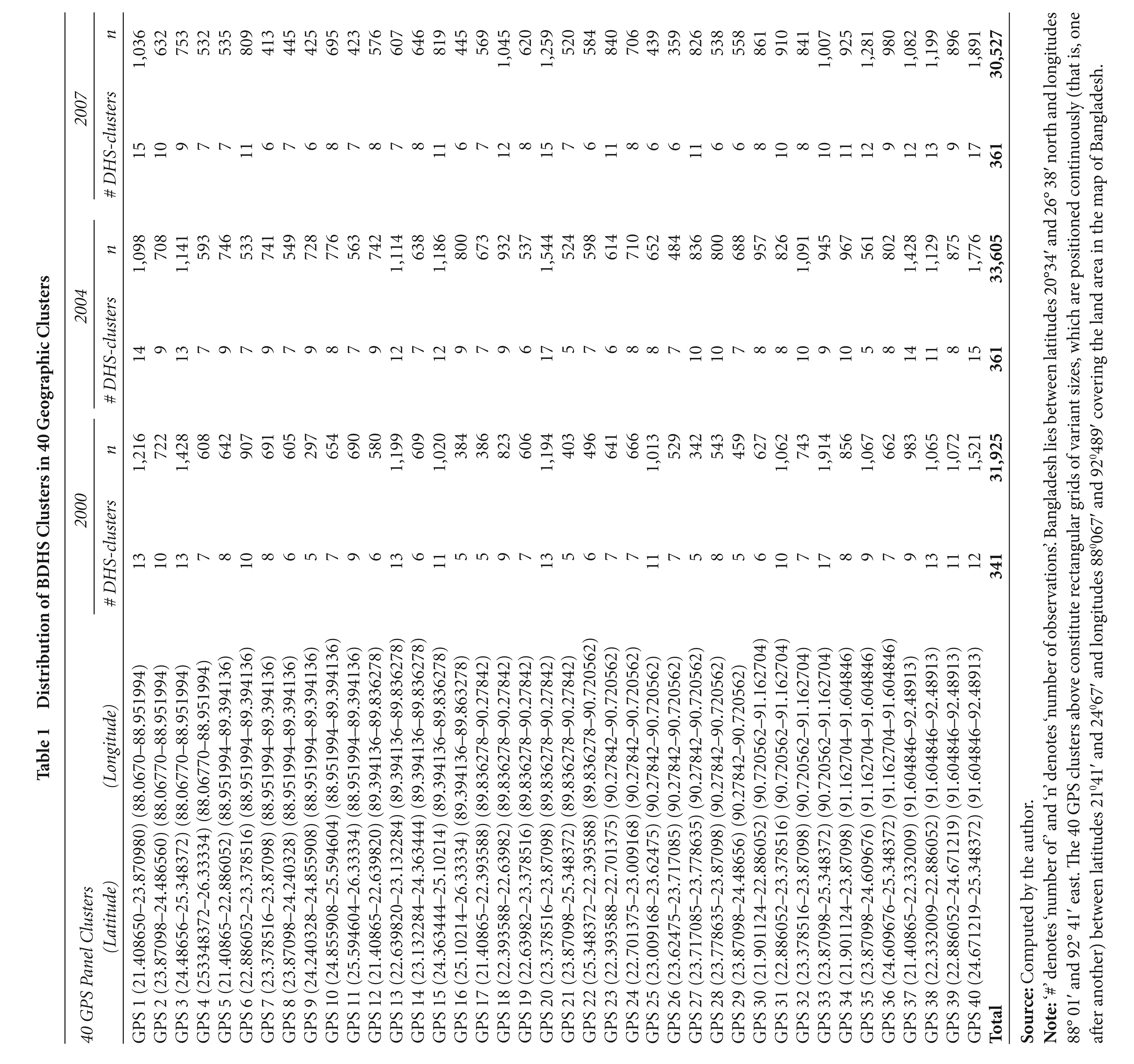
From the panel data perspective it is imperative that the 40 GPS clusters, bounded by the corresponding latitudes and longitudes remain exactly the same for all the three surveys. The number of DHS clusters lying within those GPS clusters varies across survey rounds. Table 1 presents, for each BDHS survey round, the number of DHS clusters and number of respondents (observations) within each of the 40 GPS clusters. For instance, GPS cluster 1 includes 13 clusters with 1,216 respondents from BDHS 2000, 14 clusters with 1098 respondents from BDHS 2004 and 15 clusters with 1,036 observations from BDHS 2007. None of the 40 GPS clusters include DHS clusters less than five. The total number of clusters distributed across 40 GPS clusters for successive rounds are 341 for 2000; and 361 for 2004 and 2007. The panel database thus constructed includes 120 GPS clusters from the three rounds of BDHS.
Distribution of BDHS Clusters in 40 Geographic Clusters
3.2.1 Construction of a Wealth Index
A typical DHS does not record information on the economic status of households in terms of monetary units. The DHS however records several aspects of household characteristics that essentially represent a household’s economic status. The wealth index is an attempt to make better use of existing DHS data in a systematic fashion to determine a household’s relative economic status. It has been tested in a large number of countries in relation to inequities in household income, use of health services and health outcomes (Gwatkin et al., 2007; Rutstein and Johnson, 2004).
4
However, there is a dearth of application in analytical studies in general and in those examining the health–wealth relationship in particular, using the Bangladesh DHS. Various multivariate factor analytic techniques exist to aggregate the range of wealth variables into a uni-dimensional measure of a wealth index. The most prevalent ones are principal component analysis (PCA), principal factor analysis (PFA) and multiple correspondence analyses (MCA).
5
The construction of an index of the household wealth or assets requires selecting appropriate indicators and deriving a set of weights using the PCA or PFA. The index will take the form of:

where Wi is the asset index for household i, the wik’s are the individual assets (including other indicators of living standards), k, recorded in the DHS, and
Figure 1 summarises inter-temporal performances of the geographical clusters with respect to the wealth index. The wealth indices for the geographical clusters are derived by taking the mean values of the households’ index scores. The scatter diagram Figure 1 plots the wealth indices of 40 geographical clusters for the year 2007 on the y-axis against the corresponding wealth index for the year 2000 on the x-axis. The diagonal line is the 45o line—any scatter point above the 45o line indicates that the wealth index of the corresponding cluster has improved in 2007 from its 2000 level. A similar diagram below plots the wealth indices for the year 2004 against the corresponding 2000 level. It is evident that, from 2000 to 2004, the wealth indices for 15 geographic clusters are reduced and for 1 remained unchanged, which means that two-fifths of the 40 geographic clusters could not improve their wealth situation during this time period. In 2007, 29 geographic clusters out of 40 registered an improvement in their wealth indices from their corresponding 2000 level.
Life expectancy can be defined as the number of years a baby born in a particular area or population can be expected to live if it experienced the current age-specific mortality rates of that particular area or population throughout its life. It is in essence a summary measure of mortality like any other, as it shows how long a baby would be expected to live if current age-specific mortality rates remain constant. Life expectancy is not a forecast of how long babies born will actually be expected to survive, because age-specific mortality rates are not constant over time.
Life expectancy has been calculated using the abridged life table approach (see for example, Hinde, 1998; Rowland, 2003). The BDHS survey records the birth and death history of each child born. This allows calculating the infant and child mortality rates. Mortality measures are based on deaths over a specific period of time—in this article it is in the 5 years before the survey date. The information needed from the survey is the variable indicating how old the living-child was at the date of interview; and in case of a child who had died, how old the child would have been at the interview data if the child had survived. The combination of the above two leads to measuring the survival time, which is equal to the time elapsed since birth in the case of children who are still alive; and equal to the time between birth and death in the case of children who are not alive. The relevant BDHS variables required are date of interview (v008), date of birth (b3), age at death (b7) and whether the child is still alive (b5). The mortality (for example, infant and child mortality) rates are subsequently generated by the life table information produced using the STATA statistical programme (O’Donnell et al., 2008), where the life table records the number of births, deaths and age- specific survival probabilities.

However, adult mortality rates cannot be calculated, because this requires birth and death profiling of each adult. In many of the Demographic and Health Surveys, there exist sibling histories recording their birth and deaths, which can then be used to estimate adult mortality. The BDHS does not have sibling history and therefore the age-specific adult mortality rates are taken from different sources. In short, GPS cluster-specific death rates for infant and child mortality rates are calculated using the BDHS data as described before. The age-specific probabilities of child death (up to age 5) are then used to construct the life table. Probabilities of death for above age 5 are taken from the widely used Health and Demographic Surveillance System of ICDDRB, Bangladesh (ICDDRB 2002, 2006, 2009). 6 Five-yearly interval death probabilities over age 5 for the years 2000, 2004 and 2007 are used. One important implication is that the adult mortality profiles remain constant across the 40 GPS clusters for a particular year. The variations in life expectancies across the GPS clusters are generated from the cluster-specific infant and child mortality rates. In developing countries, most of the health achievements are reflected in the improved profiles of the child and infant mortality rates, which in turn, play the most prominent roles in determining the life expectancy figures. The life expectancies at birth for the population as a whole estimated in this way are 62.43, 64.34 and 66.06 years for 2000, 2004 and 2007, respectively, which is very close to the official national estimates. 7
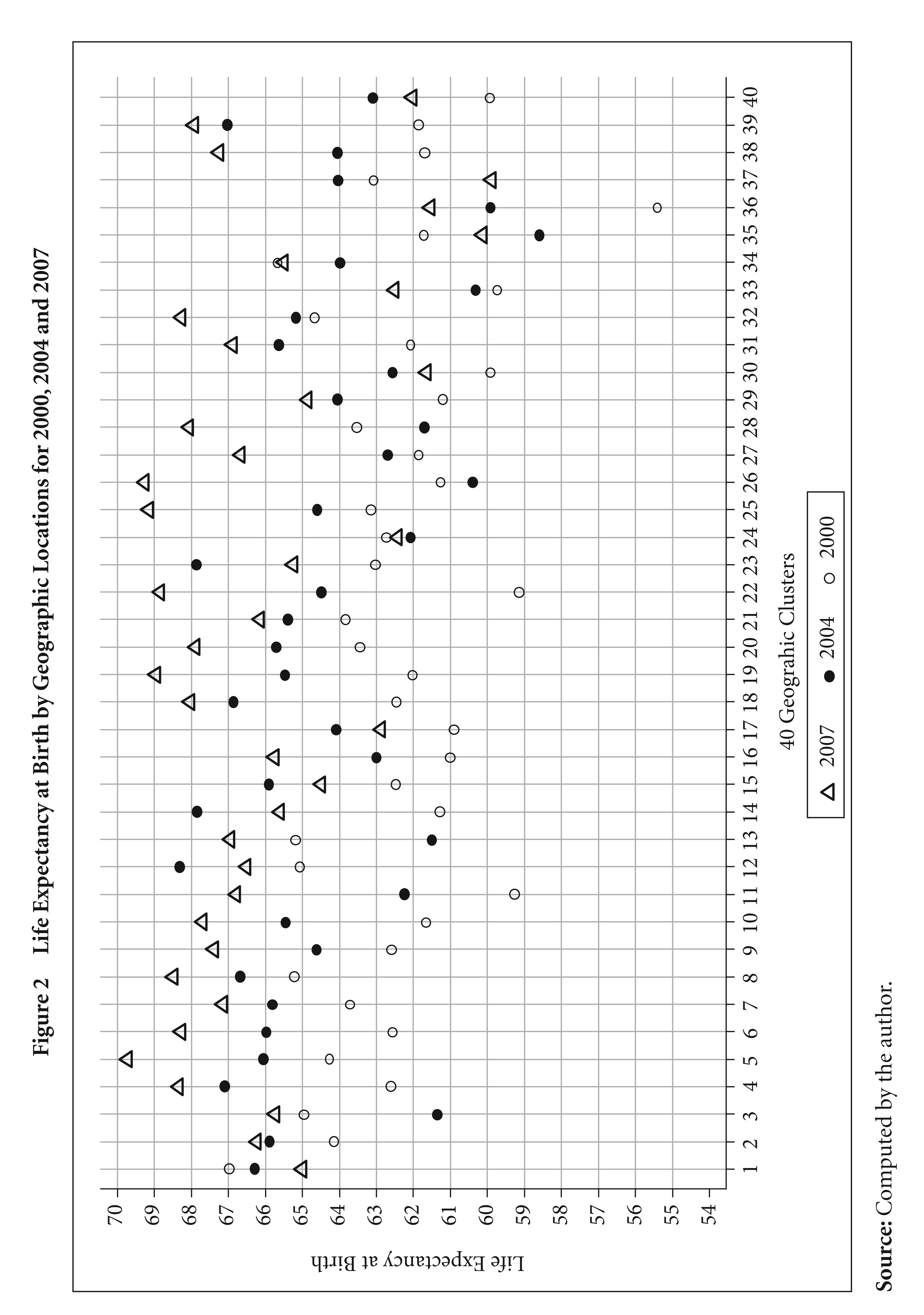
Figure 2 shows the life expectancy estimates for the 40 GPS clusters and how they performed in the three survey rounds. The graph shows improvement in life expectancy over the years, but there exist large cross-cluster variations.
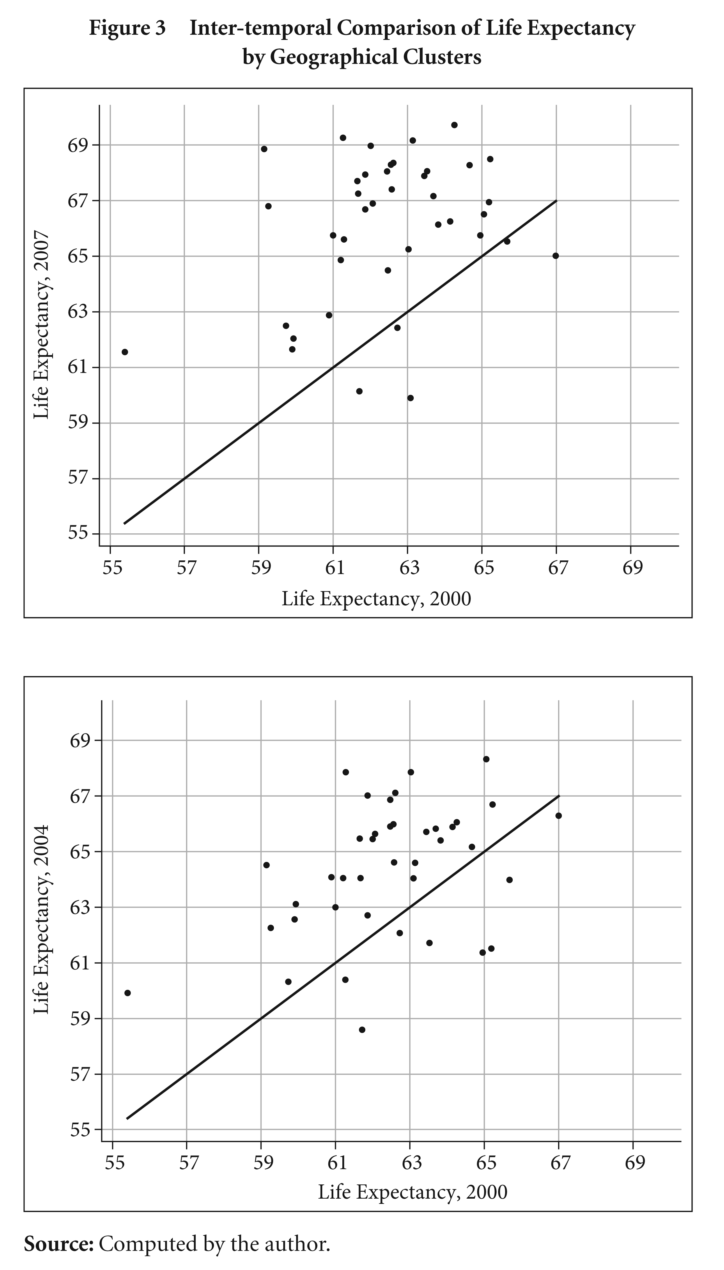
The inter-temporal comparisons of life expectancy in Figure 3 for the 40 geographic clusters show that 32 out of 40 clusters improved their life expectancies in 2004 from the 2000 level. By the year 2007, all but five geographic clusters improved their life expectancies from the corresponding 2000 levels. However, despite increases in life expectancies, there are apparently heterogeneous increments for the clusters with similar initial levels of life expectancies.
3.3 Instruments: Immunisation Coverage
Immunisation, a proven tool for controlling and eliminating life-threatening infectious diseases, is one of the most cost-effective public health interventions with demonstrated strategies that make it accessible to even the most hard-to-reach and vulnerable populations. It has clearly defined target groups; it can be delivered effectively through outreach activities; and vaccination does not require any major lifestyle change (WHO, 2003). The Expanded Programme on Immunization (EPI) launched by the World Health Organization (WHO) in 1974 increased immunisation from 5 per cent of all children to 80 per cent in a span of 30 years (Tangermann, 2007). This was mainly possible due to coordinated efforts from a coalition of partners: governments, the United Nations Development Programme, UNICEF, development agencies, the World Bank, the Rockefeller Foundation, Medecins sans Frontières, and Rotary International. Since 2000, the Global Alliance for Vaccines and Immunisation (GAVI) has been very successful at re-focusing immunisation activities globally. 8 For people in developing countries, successful immunisation programmes save thousands of lives and organisations including UNICEF and the WHO are committed to making vaccines against measles, polio and other serious diseases available to as many children as possible. The EPI initiative in Bangladesh started in 1979, with financial assistance primarily from UNICEF. Since then the EPI has experienced four phases of development. With the strong historical commitment and support from both the external sources (that is, multi-donor funding schemes) and the Government of Bangladesh, the EPI has been one of the largest recipient of funds among development projects in the health sector (Mahmud and Richard, 1998).
This article adopts the DHS definition of vaccinations rates—the percentage of children age 12–23 months who received specified vaccines at any time before the survey (Rutstein and Rojas, 2006). The numerator in this case is the number of children receiving specified vaccines, or all specified vaccines, according to information on the vaccination card or reports by respondents. The denominator is the number of living children between 12 and 23 months of age. The descriptions of the specified vaccines are the following: (a) DPT—triple vaccine for diphtheria, pertussis and tetanus, received in three doses at 6, 10 and 14 weeks after birth; (b) polio—received in three doses usually given at same time as DPT, plus at birth in some countries; (c) measles—recommended to be given at 9 months; and (d) all vaccinations—BCG, three doses of DPT, three doses of polio (excluding the dose given shortly after birth) and measles.
4. MAIN RESULTS
4.1 The Preston Curve
The joint evolution of cross-country life expectancy and income during the twentieth century in Preston’s framework suggests the modest influence of income in improving aggregate health (for example, life expectancy), albeit there are strong cross-sectional correlations (Preston, 1975). The increasing and concave Preston curves, as graphed with cross-country data for consecutive decades, shifted upward or rightward over time. This rendered fallacious the conventional conjecture about the dominant impact of income on health. An upward shift of the curve means countries achieve increases in life expectancy without increases in the GDP per capita. A rightward shift on the other hand would imply countries not increasing their life expectancy despite increments in GDP per capita.
Figure 4 shows the scatter plot of life expectancy at birth and the wealth index as derived from the regional profile. There is a prominent upward shift, accompanied by a moderate rightward shift, of the linear-fit curve from 2000 to 2007 indicating a large improvement of population health associated with a small change of wealth status. The shapes resemble the ones generally obtained from the scatter plots using cross-country life expectancy and income per capita data. As in the case of macro-level scatter plots, the GPS cluster-level scatter also indicates that some clusters registered high increase in the wealth index but relatively performed poorly in increasing life expectancy. This would contribute to the rightward shift of the curve. These shifts of the curve indicates the existence of exogenous drivers of health and a large-scale immunisation programme may be significant factors in this regard.

4.1.1 Regression Results
This article uses unobserved effects model to quantify the impact of health improvements on economic well-being, proxied by the wealth index. Both the region (that is, geographical cluster) and time-fixed effects are included in the specification. The unobserved effects for each geographical cluster control for omitted variables that are constant over time but differ across entities and the time-fixed effects control for variables that are constant across entities but evolve over time. However, if either of the combined region-fixed effects, or the combined time-fixed effects in particular, are found to be statistically insignificant these fixed effects may be dropped from the model specification.
In empirical work with panel data, there exists concern whether one should allow for correlation between the unobservable heterogeneity and the regressors. Since the within-group (WG) estimator eliminates the unobserved heterogeneity by taking mean deviations of variables prior to estimation by OLS, it is consistent regardless of whether the unobserved effect zg and the observed health variable are correlated or not. On the other hand, the generalised least squares (GLS) estimator is only consistent under the assumption that the unobservable zg is uncorrelated with the regressors in the model. In presenting the results, this article reports the estimates using both the WG estimator as well as the GLS, including and excluding time effects in the specification. The reported standard errors are robust adjusting for GPS clusters (see Wooldridge, 2002, p. 275). Therefore, the standard errors allow for intra-region correlation, relaxing the usual requirement that the observations be independent. In other words, the observations are independent across GPS clusters but not necessarily within GPS clusters. Also, the model is estimated using WG and GLS estimations (with or without time effects).
4.1.2 First Stage Estimates: Vaccination and Health
Different vaccination rates are used as instruments for the health outcome (that is, life expectancy). Because of the presence of very high collinearity between the various vaccination rates, they are used separately to examine the impact on health outcomes. Figure 5 shows the reduced form relationship between the change in vaccination coverage (all vaccines) and the change in life expectancy between the years 2000 and 2007. The linear fit suggests positive correlations. There are some atypical clusters, for example cluster 37, where the positive change in the immunisation coverage is associated with a negative change in life expectancy. This cluster is adjacent to the coastal area and more prone to tropical cyclones; and this may partially explain the increased death toll and thereby decreased life expectancy for this area.
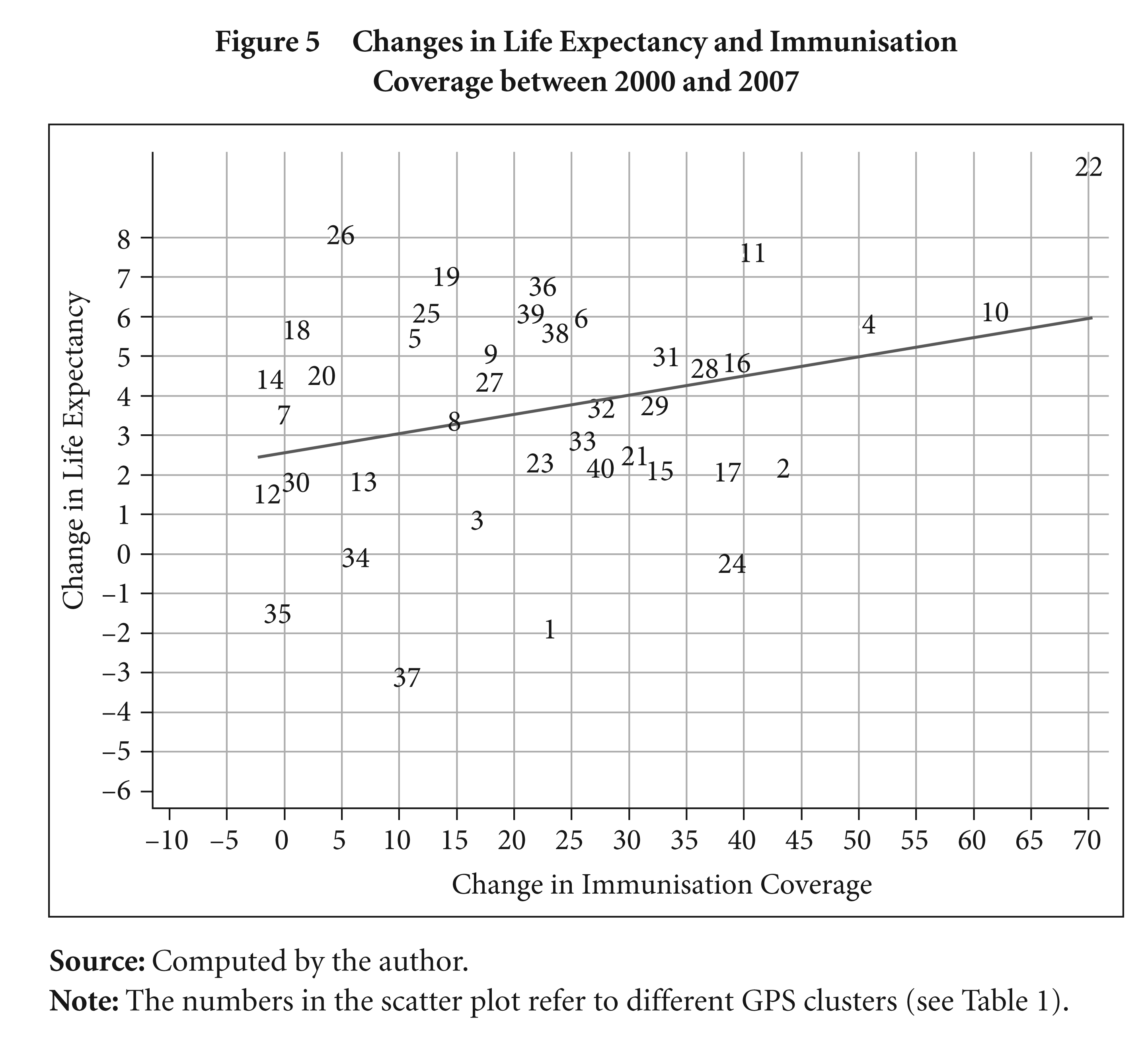
Figure 6 shows the reduced form relationship between the change in the wealth index and the change in vaccination coverage. The scatter plot and the linear fit suggest no correlation between the two and that the vaccination coverage for majority of the GPS clusters registered a sharp increase irrespective of the direction of the changes in the wealth index. This provides robust grounds for using the vaccination coverage as an instrument to track the exogenous health outcomes and consequently its impact on the wealth index.
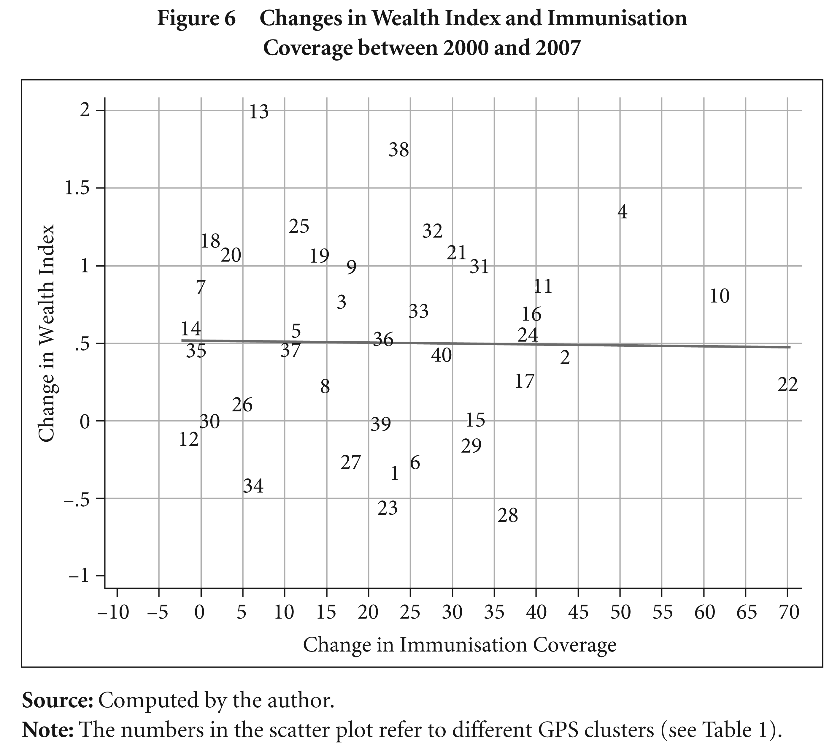
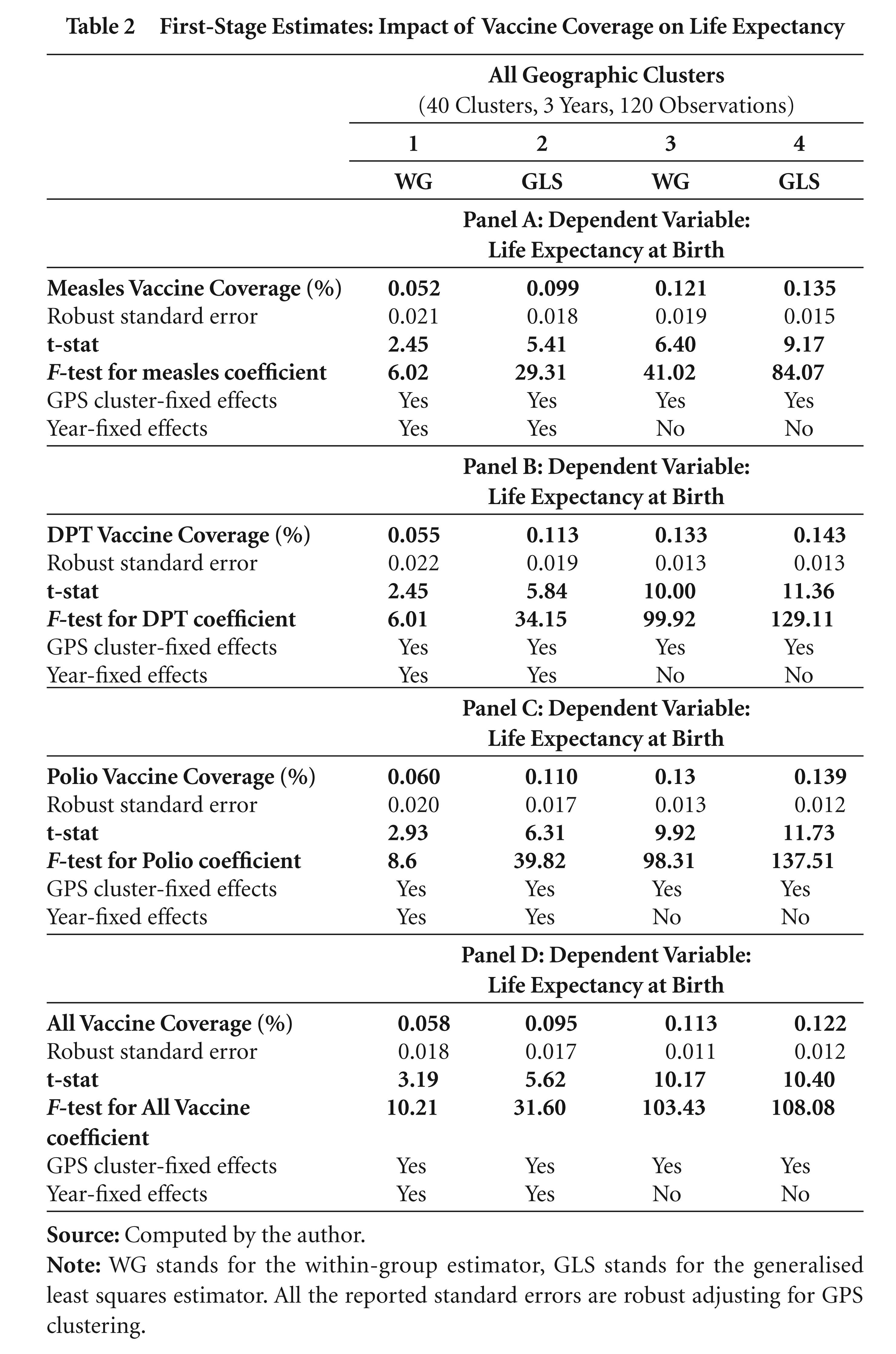
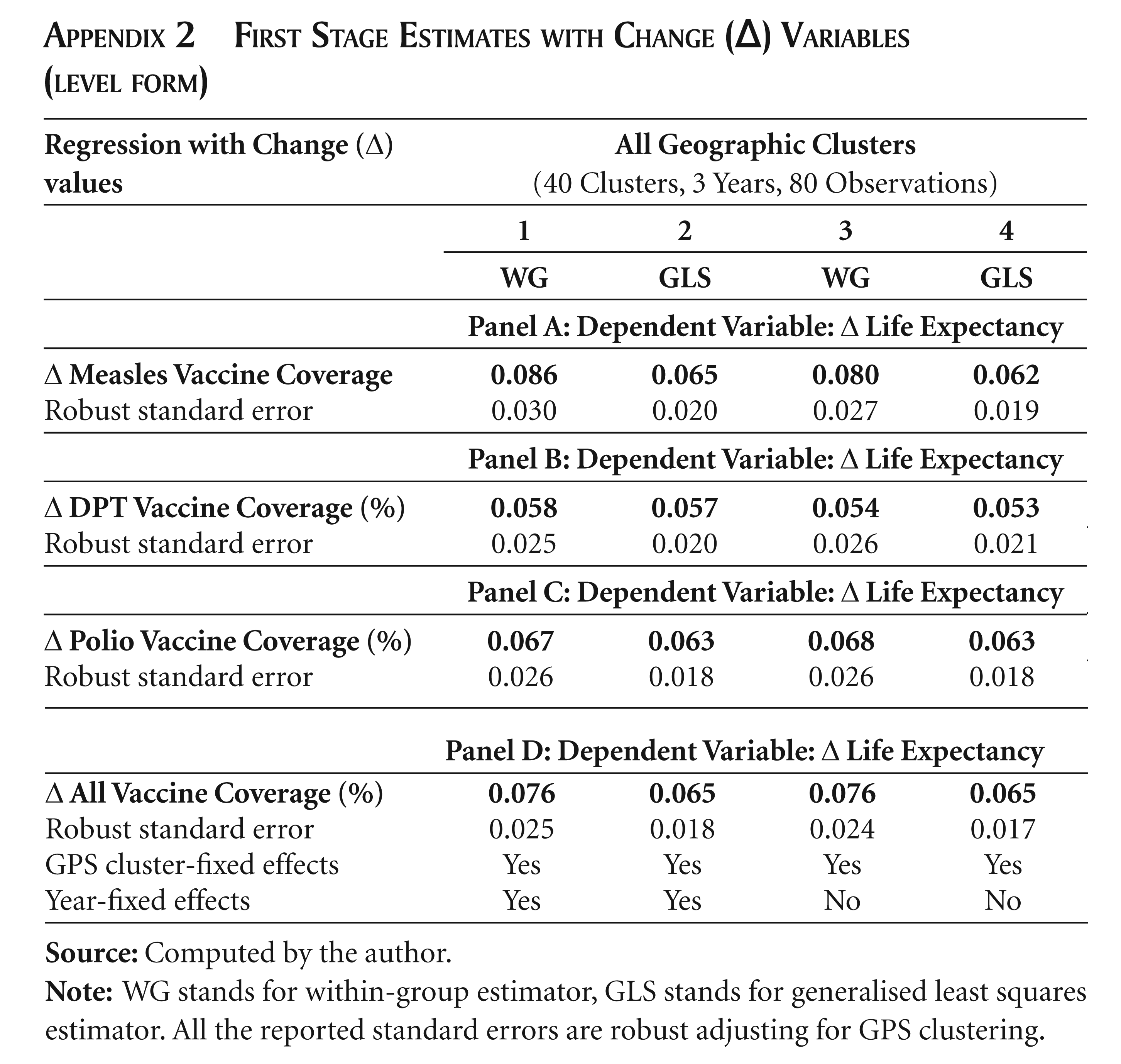
Table 2 presents the first-stage estimates with regards to the impact of measles, DPT, polio and all vaccines coverage on life expectancy, respectively. There are four panels (A–D) reporting the results of the impacts of corresponding vaccination rates on life expectancy. A highly significant coefficient with high F-statistics above 10 would qualify as a good instrument (Stock and Watson, 2006). For instance, panel A in Table 2 reports the impact of measles vaccine coverage on life expectancy. The mean value of the coefficient for all the 4 specifications is 0.102, implying a 10 per cent increase in measles vaccination coverage was associated with a 1.02 year increase in life expectancy. All the coefficients are statistically significant. In general, the reported coefficients and the test statistics validate the vaccine variable as a good instrument for explaining life expectancy. Appendix 2 presents the first- stage estimates when the ‘change’ variables are used, that is, the impact of the change in the vaccination rates on the change in life expectancy. The coefficients again are all statistically significant.
First-Stage Estimates: Impact of Vaccine Coverage on Life Expectancy
4.1.3 2SLS Estimates: Contribution of Life Expectancy to Wealth
Table 3 presents the two-stage least square (2SLS) estimates of the effect of life expectancy on wealth status obtained from the log specifications to show the elasticity values. Similar to the previous table, the regression specifications are estimated using WG and GLS estimators and with and without time-fixed effects. Table 3 reports a total of 16 coefficients in four panels for the log life expectancy indicating the percentage increase in the wealth index due to a 1 per cent increase in life expectancy.
The elasticity values for the four specifications in panel 1 when measles coverage has been used as an instrument range from 1.596 to 2.555, with a mean value of 2.16. This implies that a 1 per cent increase in life expectancy would lead to an increase in the wealth index of 2.16 per cent. The joint test for time effects are insignificant and after excluding them in the specifications generate higher and significant elasticity values.
Panel 2 in Table 3 shows the results of 2SLS estimates of the impact of life expectancy on the wealth index when DPT vaccine is used as the instrument for life expectancy. The estimated coefficients are relatively more significant and larger across specifications with a mean elasticity value of 3.48, implying that a 1 per cent increase in life expectancy leads to an increase in the wealth index by 3.48 per cent. Time effects are again insignificant under both WG and GLS specifications. The specifications without time effects and/or using the GLS estimator generate highly significant estimates of the elasticity values. These results assert the positive impact of health on wealth.
Similar evidence can be observed in panel 3 when polio vaccine coverage has been used as the instrument. However, somewhat contrasting evidence emerges when ‘all vaccine’ coverage is used as an instrument. The WG and GLS estimates are insignificant when time effects are included and are statistically significant at the 10 per cent level of significance. The elasticity values are 2.07 and 2.23 under the WG and GLS specifications without time effects, respectively. However, there is some caution to be exercised while using the ‘all vaccine’ variable. By construction, only the areas where all the vaccine routines are implemented are accounted for. There might be some GPS clusters where the vaccination rates for most of the vaccine routines are quite high and yet miss out on one vaccine leading to a significantly lower mean value for the ‘all vaccines’ coverage. Therefore one might expect slightly larger variations in cross-cluster ‘all vaccine’ rates.
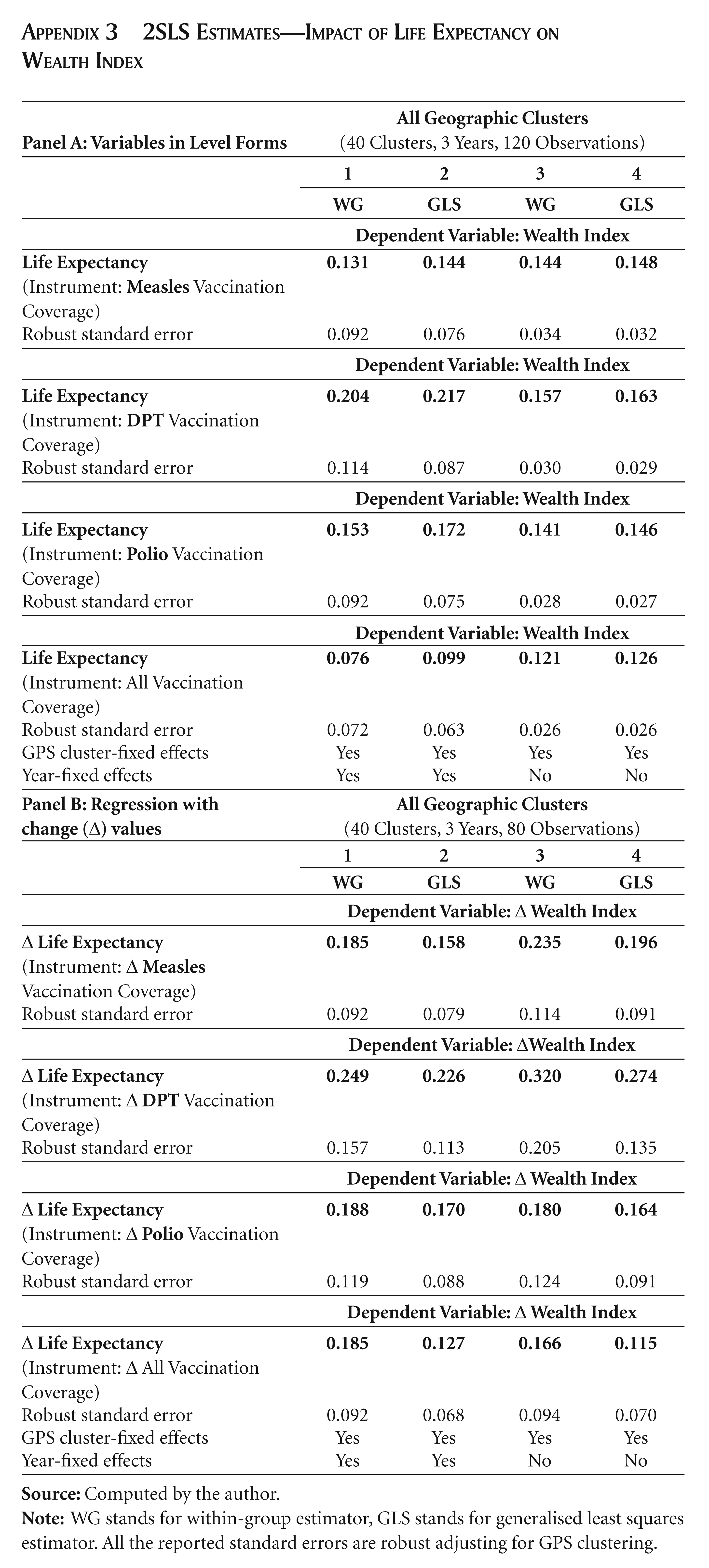
2SLS Estimates: Impact of Life Expectancy on the Wealth Index

Appendix 3 presents some supplementary regression results, where panel A shows the coefficients when the variables are used in level forms and panel B shows the coefficients when the changes in the respective variables are used in the regression. The estimated coefficients in the upper panel are more or less in concordance with those in the lower panel.
5. CONCLUSION
The estimates in general suggest a sizeable, positive, robust and in most cases significant impact of life expectancy on economic well-being captured by the wealth status. The within-country GPS cluster-level heterogeneity with respect to the health and wealth indicators and their evolution over time provides useful insights. The positive elasticity values obtained from this within-country cluster-level analysis corroborates the findings of several macro regression studies. 9 The findings promote the concept of investing in health, which would foster achieving the health objectives of the country (for example, the Millennium Development Goals), as well as boost economic well-being. Also, the estimates of the impact of health on wealth correspond to the time span of only seven years (that is, from 2000 to 2007). It may be expected that the full impact will be realised in the longer run which then could further validate the positive, significant and sizeable impact of life expectancy on economic well-being.
Footnotes
CONSTRUCTION OF THE WEALTH INDEX
In the construction of the wealth index, the variables included and the weights obtained from the first principal component and the first principal factor are presented in Appendix Table 1. The bottom panel of the table provides the respective eigenvalues (for example, 7.41 and 7.23) and proportion of variances explained (20 per cent and 24 per cent). 10 The weights are assigned for each category of variables. It should be noted that some indicators are assigned positive weights and some are assigned negative weights. Generally, a variable with a positive factor is associated with higher socioeconomic status and conversely a variable with a negative factor score is associated with a lower living standard or socioeconomic status (Vyas and Kumaranayake, 2006). This is evident from the weights in the table. The possession of durable goods carries positive weights (compared to non-possession); the worse housing characteristics are assigned negative weights and a household whose members have low education is assigned negative weights. Using these weights, the factor scores (that is, wealth index) are derived for each household. It is expected that the lower the score, the lower the living standard; and vice versa.
One of the advantages of using a wealth index is that for inter-temporal and intergenerational comparisons, we need not rely on doubtful price deflators that are used to compare monetary measures of living standards (Sahn and Stifel, 2000). This article makes inter-temporal comparisons of this wealth index and in that case, it is necessary to construct wealth indices that are comparable over time. This can be done either by pooling the data from all the DHS rounds and then estimating the PCA, PFA, or MCA scoring coefficients (that is, asset weight) for the pooled sample; or by using ‘baseline’ weights obtained from the first period. This study pooled the data from all the BDHS rounds and then created the wealth index using a common subset of wealth indicators appearing in each survey, so that the index is comprised of exactly the same indicators for each survey.
The wealth indices derived under the PCA, PFA and MCA were found to be highly correlated (above 0.98), as expected. Therefore, this article presents all the results based on the wealth index generated using the PCA method. Since the wealth index contains negative values and positive values, the log transformation of the wealth index is not feasible. In order to define the distribution of the wealth index over positive real numbers, a value equal to the largest negative value in the index was added to each of the indices (following Asselin, 2002; Sahn and Stifel, 2003), so that the lowest observed value becomes zero. This would only shift the distribution preserving the variances but not the means; and would not affect regression coefficients applied at the level forms. Appendix Figure 1 shows the evolution of the distribution of the wealth index at the household level over the three rounds (2000, 2004 and 2007). The shape of the distribution became relatively flatter in successive rounds indicating betterment in the living standard.
FIRST STAGE ESTIMATES WITH CHANGE (∆) VARIABLES (LEVEL FORM)
|
|
(40 Clusters, 3 Years, 80 Observations) |
|||
|
|
|
|
|
|
|
|
|
|
|
|
|
|
||||
|
|
|
|
|
|
| Robust standard error |
0.030 |
0.020 |
0.027 |
0.019 |
|
|
||||
|
|
|
|
|
|
| Robust standard error |
0.025 |
0.020 |
0.026 |
0.021 |
|
|
||||
|
|
|
|
|
|
| Robust standard error |
0.026 |
0.018 |
0.026 |
0.018 |
|
|
||||
|
|
|
|
|
|
| Robust standard error | 0.025 | 0.018 | 0.024 | 0.017 |
| GPS cluster-fixed effects | Yes | Yes | Yes | Yes |
| Year-fixed effects | Yes | Yes | No | No |
2SLS ESTIMATES—IMPACT OF LIFE EXPECTANCY ON WEALTH INDEX
|
|
(40 Clusters, 3 Years, 120 Observations) |
|||
|
|
|
|
|
|
|
|
|
|
|
|
|
|
||||
|
|
|
|
|
|
| Robust standard error |
0.092 |
0.076 |
0.034 |
0.032 |
|
|
||||
| 0.204 | 0.217 | 0.157 | 0.163 | |
| Robust standard error |
0.114 |
0.087 |
0.030 |
0.029 |
|
|
||||
| 0.153 | 0.172 | 0.141 | 0.146 | |
| Robust standard error |
0.092 |
0.075 |
0.028 |
0.027 |
|
|
||||
| 0.076 | 0.099 | 0.121 | 0.126 | |
| Robust standard error | 0.072 | 0.063 | 0.026 | 0.026 |
| GPS cluster-fixed effects | Yes | Yes | Yes | Yes |
| Year-fixed effects |
Yes |
Yes |
No |
No |
|
|
||||
|
|
|
|
|
|
|
|
|
|
|
|
|
|
|
|||
| 0.185 | 0.158 | 0.235 | 0.196 | |
| Robust standard error |
0.092 |
0.079 |
0.114 |
0.091 |
|
|
|
|||
| ∆ Life Expectancy |
0.249 | 0.226 | 0.320 | 0.274 |
| Robust standard error | 0.157 | 0.113 | 0.205 | 0.135 |
|
|
|
|||
| 0.188 | 0.170 | 0.180 | 0.164 | |
| Robust standard error |
0.119 |
0.088 |
0.124 |
0.091 |
|
|
|
|||
| 0.185 | 0.127 | 0.166 | 0.115 | |
| Robust standard error | 0.092 | 0.068 | 0.094 | 0.070 |
| GPS cluster-fixed effects | Yes | Yes | Yes | Yes |
| Year-fixed effects | Yes | Yes | No | No |