Backtesting of Value at Risk Methodology: Analysis of Banking Shares in India

Abstract

Value at risk (VaR) is used by financial experts to calculate and predict the risk of financial exposure. In the presence of volatility and long memory, it is a model useful for the prediction of loss in the equity index return series. Checking the accuracy of this model is necessary from the practitioners’ point of view. This article initially checks the presence of autoregressive conditional heteroscedastic (ARCH) and long-memory effects in the daily closing price of the Bombay Stock Exchange (BSE)-BANKEX return series. After confirming the ARCH and long-memory presence, it analyses the different methods of VaR calculation such as asymmetric power ARCH (APARCH), fractionally integrated exponential generalised ARCH (FIEGARCH), hyperbolic generalised GARCH (HYGARCH) and risk metrics. Then, it empirically tests the forecasting capacity of these VaR methods through techniques such as the Kupiec likelihood ratio (LR test) and dynamic quantile test. Furthermore, it checks the root-mean-squared error (RMSE) and mean absolute error (MAE) to determine the model with the least error. From the set of VaR models used here, by and large it concludes that the BANKEX return series has both long-memory and asymmetry effects. By comparing these models, it is implied that the HYGARCH model gives a better result, although the other models have their significance in the estimation and forecasting of the BANKEX return series.

JEL: C12, D81, C530

Keywords

Value at Risk Backtesting BANKEX Asymmetric Volatility Long Memory

1. INTRODUCTION

Value at risk (VaR) is a tool used in financial engineering to calculate the possible maximum loss from any financial position based on historical data. It can also be defined as a technique used to estimate the maximum portfolio losses for a given probability level from any financial risk or uncertainty position using historical data trend and volatility study. The VaR method is mainly used by banks that came to the forefront with the introduction of the internal model (1996) for market risk in the Basel I framework, and is also used for other risk measurements such as credit, operations and liquidity risk. The use of this concept has been extended from bankers to other financial agents such as financial business analysts, security firm investors and trading agents who usually deal with the risk-taking behaviour. It measures the maximum amount of loss that a financial firm can face when it decides to do trading or hedging. It helps investors and credit givers to analyse risk-taking behaviour and map the maximum loss.

There are different methodologies to estimate VaR. The most widely used are the historical simulation and Monte Carlos simulation techniques. Apart from these, several other asymmetry and long-memory models are used by financial experts, who believe that the return series of exposure has asymmetry and a long-term dependence on past returns.

With the extensive use of various VaR models, verification of the accuracy of these models became necessary for financial experts to determine which best forecasts VaR. The long-memory VaR models have been empirically analysed by McMillan and Thupayagale (2010) based on South African stock returns and using the asymmetric and long-memory models. Accuracy has been checked by backtesting the VaR forecasts and it is found that both the asymmetric and long-memory methods for VaR calculations give better results; in particular, the fractionally integrated exponential generalised autoregressive conditional heteroscedastic (FIEGARCH) gives the better result for daily VaR with a 99 per cent confidence level.

There have been several studies in India on VaR models, such as Varma (1999) on the Nifty Index of the Indian share market, Dutta and Bhattacharya (2008) on the CRISIL NSE Index (CNX) Nifty using the bootstrapped historical simulation VaR model and Sarma, Thomas and Shah (2003) using different VaR models from the forecast point of view in the Indian share market. However, studies on the backtesting of VaR models, which have become vital after the global financial crisis (GFC) are less evident in India, and the present study is an attempt in that direction. Most of the studies in India are done with the BSE-Sensex or the NSE-Nifty; however, the current study tries to analyse the sectoral index of the BSE separately. The BSE-BANKEX has been selected for this study over other sectoral indices, with the aim of studying the index with the highest trading volume among BSE sectoral indices. The BSE-BANKEX¹ is composed of 12 banks representing the Indian banking industry, and this composition is determined by the BSE sectoral industry classification norm. However, for other particular sector analyses, the different sectoral indices may be taken into account.

With this background, the current article studies both asymmetry and long-memory VaR models for analysing Indian bank shares. Stationarity is checked and confirmed for the BSE-BANKEX return series by using unit root tests such as the Augmented Dickey–Fuller (ADF) and Phillips–Perron (PP) tests. Further, the return series is tested using the Lagrange multiplier ARCH (LM ARCH) test to verify the presence of an ARCH effect, and the Hurst–Mandelbrot test and Lo test to check for the presence of long memory before it is used for estimating VaR models. These tests confirm the presence of the ARCH effect and long memory in the BANKEX return series. The used asymmetry and long-memory VaR models for this study are risk metrics, the asymmetric power ARCH (APARCH) model, the FIEGARCH and the hyperbolic generalised ARCH (HYGARCH) model. These VaR models are estimated for analysis and their significance level is also checked. Then, they are verified for accuracy with backtesting techniques such as the Kupiec LR test and the dynamic quantile test. Furthermore, for forecast evaluation the mean absolute error (MAE) and root-mean-squared error (RMSE) statistic are used. The model with the minimum error is considered to have the best forecast capacity.

The rest of the article is as follows. Section 2 discusses the existing literature on the VaR methodology and its backtesting. Section 3 presents the data and methods used in this article. The estimated empirical results are analysed in Section 4, Section 5 discusses the GFC and Section 6 concludes the article.

2. LITERATURE REVIEW

There have been extensive studies on the VaR and its application in measuring the maximum possible loss in the financial system. Testing the efficiency of VaR models is essential and needs to be practiced. This can be done through backtesting of the model estimated, a practice that the Bank for International Settlements (BIS) has been continually promoting. It is a process where we go back to the data and check whether the estimated results are reflecting in our data or not. The backtesting technique is being applied in several countries using sophisticated methods, and developing countries such as India need to follow the example.

The accuracy of VaR forecast is crucial, as it is used as a benchmark on how much capital needs to be preserved as per the regulator’s requirements. Berkowitz and Obrien (2002) have made a detailed study of the accuracy of VaR models in the trading book account of large-size banks in the US, and found that banks are reporting conservative VaR, which forces them to keep higher levels of capital coverage for trading books.

The choice of VaR methodology should be left to efficient users of the VaR model and the sector for which VaR is to be calculated. Sarma et al. (2003) analysed the Indian share market by using different VaR models from a forecasting point of view and found that the VaR models give varied results. Users should choose alternative VaR models for different portfolio VaR estimations. Similarly, Bucevska (2013) studied various types of VaR models in the Macedonian stock exchange and found that the asymmetric model EGARCH, with a student t distribution, gives a better result than other GARCH family models. Gourieroux, Laurent and Scaillet (2000) conducted a sensitivity analysis on changing the portfolio which helps identify an efficient model, and it used dynamic VaR techniques for estimation of the risk.

The presence of long memory also plays a crucial role in the calculation of VaR. The calculation of VaR through long-memory models outperforms other VaR estimation models. The Malaysian equity market has been studied by Manap and Kassim (2011) with respect to the presence of long memory, and they find the presence of long memory as well as asymmetry in the Kuala Lumpur Stock Exchange (KLSE). Furthermore, Ho, Shi and Zhang (2013) have used firm-level stock return data for VaR analysis through a long-memory (FIGARCH) and regime-switching GARCH (RS-GARCH) model and found long-memory models to be more useful for VaR analysis than the RS-GARCH. In the same line, Wang, Bauwens and Hsiao (2013) analysed the long-memory VaR models with structural breaks and found that their new way of estimating VaR shows better results than their previous estimation methods. Another study on long memory was done by Floros, Jaffry and Lima (2007) in the Portuguese stock market where they examined the long memory by taking two periods of data for analysis, merger and post-merger of the Portuguese Stock Exchange with Euronext, and discovered the presence of long memory in the Portuguese Stock Exchange for both periods. However, after the merger, weak long memory is observed, implying that the market has become more efficient after the merger.

Long-memory VaR can also be used for other data analysis except for the stock return series. Aloy, Dufrenot, Tong and Feissolle (2012) have studied long-memory VaR models by using the non-linear least square method for the analysis of unemployment data.

The VaR method has been severely criticised in the aftermath of the GFC. It was claimed that the VaR technique is one of the reasons responsible for the GFC. This is based on several assumptions, which is a problem for real estimation of the loss, because with the increase in the number of assumptions, the probability of accuracy of the results decreases. For the sake of accuracy, the VaR models need to be regularly backtested, and alternative models should be considered (Blanco & Oks, 2004).

With the availability of these varied relevant VaR models, choosing the best VaR model to provide accurate VaR estimates has become highly critical. Backtesting is one of the tools used to check the accuracy of the estimated VaR model. Huang and Tseng (2009) examined the forecast of the VaR models for both developed and emerging market economies and found that non-parametric VaR models perform better in forecasting VaR compared to other VaR models.

3. DATA AND METHODOLOGY

The daily closing price of the BSE-BANKEX for the period 1 April 2003 to 31 March 2014 has been selected from the Centre for Monitoring Indian Economy (CMIE) to study the VaR methodology. The calculation of the VaR model is done by using the daily return as

p_tp_t_–1

where (p_t) represents the closing price of BANKEX at period t.

The ADF and PP tests are used for stationarity analysis. The LM ARCH test and long-memory tests such as the Hurst–Mandelbrot test and the Lo test are done to confirm the presence of the ARCH effect and long memory in the return series. Models such as the APARCH, exponential GARCH model with long-memory process (FIEGARCH), long-memory GARCH model with integration (HYGARCH) and risk metrics are used to estimate the VaR.

The estimated VaR results have been backtested using backtesting techniques such as the Kupiec LR test (1995) and the dynamic quantile test (2004). Further, for forecast evaluation, error values like the MAE and RMSE are seen to check the model with less prediction error. A brief summary of the tests performed and VaR estimation models used in this article are analysed as follows.

3.1 The LM ARCH Test

A time series variable that is uncorrelated with its past can be dependent on it due to the dynamic conditional nature of the return series. Return time series data showing the presence of conditional heteroscedasticity is said to have ARCH effects among its returns series. Engle’s (1982) Lagrange multiplier (LM) test is used to assess the presence of the ARCH effect. The null hypothesis of the ARCH effect test can be expressed as:

σ_{t}^{2} = ω + \sum_{i =1}^{q} α_{i} + U_{t,}

(1)

where U_t is a white noise error series and α_i is zero. It results show no ARCH effect is seen, and the rejection of the null hypothesis confirms that the return series has ARCH effects.

The tests of long memory confirm the presence of long-run dependence of the return series. The two long memory tests, the Hurst–Mandelbrot test and the Lo test, are used here for checking the presence of long memory.

3.2 Mandelbrot’s Rescaled Range Statistics

Mandelbrot (1972) used the rescaled range (R/S) method developed by Hurst to measure the degree of long-term dependence. Mandelbrot’s R/S statistics measures the long-term relationship mainly in non-periodic cycles. The rescaled range or R/S statistic is formulated by measuring the range of the maximum and minimum distances of the cumulative stochastic random variables. The stochastic random variable is formed by subtracting the random variable from its mean and then dividing it by its mean. It can be explained by a series say $X_{1}, X_{2}, … . X_{n},$ which has a sample mean X and standard deviation of σ_n.

The (R/S) statistic (Q_n) can be expressed as

Q_{n} = \frac{1}{σ_{n} .} [MAX \sum^{​} {(X}_{j} - X) - MIN \sum^{​} {(X}_{j} - X)] .

(2)

The null hypothesis of this test statistic says that there is no long-term dependence among the return series. The rejection of the null hypothesis indicates the presence of long memory in the return series.

3.3 Lo’s Modified Rescale Statistics

Lo (1991) pointed out that Mandelbrot’s R/S statistic may be significantly biased when there is short-term dependence in the form of heteroscedasticity or autocorrelation. Assaf (2002) suggested the use of the modified R/S statistic to avoid this issue, and it can be expressed as

Q_{n,q} = \frac{1}{{\hat{σ}}_{n}} (q)[MAX \sum^{​} {(X}_{j} - X) - MIN \sum^{​} {(X}_{j} - X)] .

(3)

The difference between the earlier R/S and Lo’s modified statistic is the denominator (Assaf, 2002a),

where ${\hat{σ}}_{n} (q)$ = $σ_{n}^{2} + 2 \sum_{j=1}^{q} w_{j} (q) \tilde{γ_{J}}$ and where w_j (q) = (1 – j)/(q + 1) and $\tilde{γ_{J}} = 1/n[\sum_{i=j+1}^{n}$ (X_i – X)(Xi – j – X)] for q < n.

Lo (1991) provides the detailed assumptions and formation for Q_n,q.

The null hypothesis is same as Mandelbrot’s test, that there is no long memory, and the rejection of the null hypothesis indicates the presence of long memory.

3.4 Asymmetric Power ARCH

The APARCH model captures the asymmetry effect, that is, volatility tends to increase when returns are negative compared to positive returns of the same magnitude. Ding, Granger and Engle (1993) introduced the APARCH model, which is expressed as:

σ_{t}^{δ} = ω + \sum_{i =1}^{q} α_{i} {(| ε_{t - i} | - γ_{i} ε_{t - i} L)}^{δ} + \sum_{j =1}^{p} β_{j} σ_{t - j}^{δ,}

(4)

where δ > 0 and −1 γ < 1 (i = 1….q).

The parameter δ plays the role of Box–Cox transformation of σ, while γ reflects the leveraging effect. This model also takes fat tails of the return series into account vis-à-vis the leveraging effect.

3.5 FIEGARCH (p, d, q) Model

The FIEGARCH (p, d, q) model is a long-memory version of the EGARCH model that was proposed by Bollerslev and Mikkelsen (1996) to capture long memory in asset-return volatility. Formation of the FIEGARCH model is done with the combination of the FIGARCH and EGARCH approaches, where both the long-memory volatility and asymmetries are modelled. Long-memory (fractionally integrated) models are those models where volatility is persistent and mean reverting (Poon, 2005).

The EGARCH model was expressed by Nelson (1991) as

g (ε_{t}) = θ ε_{t} + γ [| ε_{t} | - E (| ε_{t} |)],

(5)

where θ and γ are real constants, $ε_{t}$ and $| ε_{t} | - E (| ε_{t} |)$ are zero mean independent and identically distributed (i.i.d) sequences with continuous distributions. The $E (g | ε_{t} |)$ = 0.

The asymmetry of $g {(ε}_{t})$ can be written as

g {(ε}_{t})= {\begin{matrix} (θ + γ {)ε}_{t} - γ E (| ε_{t} |), i f ε_{t} \geq 0 \\ (θ - γ {)ε}_{t} - γ E (| ε_{t} |), i f ε_{t} <0 \end{matrix} .

(6)

The FIEGARCH model incorporating the FIGARCH model may be expressed as

\log (σ_{t}^{2})= ω + θ {(L)}^{- 1} {(1 - L)}^{- d} | 1+ α (L) | g {(ε}_{t - 1}),

(7)

where d is the long-memory (fractionally integrated) parameter.

3.6 The HYGARCH Model

The long-memory HYGRCH model (Davidson, 2004) is better at estimating unexpected announcements from the stock market. This model has the advantage of taking into account news reports while calculating the VaR for stock returns. This model is used for factoring in bad news, and it is superior to other long-memory models as it can surpass the restriction of unit amplitudes.

The HYGARCH model can be written as

σ_{t}^{2} = ω [1 - β {(L)}^{- 1}]+1 - [1 - β {(L)}^{- 1}]φ(L){1+ α [(1 - L)^{- d}]},

(8)

where φ indicates the presence of the hyperbolic component in the GARCH process. The model estimates the volatility with both long-memory and unit amplitude restriction presence and does not behave oddly when the long-memory component (d) is approximated to one. Here the amplitude parameter φ≥0 and long-memory parameter is also d ≥ 0.

3.7 RiskMetrics Model

The RiskMetrics model, first propounded by J.P. Morgan (1996) to calculate the VaR in market risk, is now being used to measure risk in liquidity and credit and operational risk. It is equivalent to a normal integrated GARCH (IGARCH) model where the ARCH and GARCH coefficients are fixed in nature.

It can be expressed as

σ_{t}^{2} = ω + α r_{t - 1}^{2} + β σ_{t - 1}^{2},

(9)

where ω = 0, $α + β =1, β$ is defined as 0.94, $σ_{t}^{2}$ is the estimated or forecast variance and r_t is the continuously compounded return series and smoothing parameter. A significant β parameter implies the persistence of forecasted volatility that can be used for VaR measurement.

3.8 Backtesting of the VaR Forecast

Accuracy of the VaR model is essential as it has a lot of control over investors’ decisions. The backtesting methodology is used to check the extent of accuracy of the forecast of the VaR model. The two tests, the Kupiec LR test and the dynamic quantile test, are used here for this verification.

3.8.1 The Kupiec LR test

The Kupiec LR test (1995), popularly known as the proportion of failure (POF) test, is conducted to verify the frequency of loss when it exceeds the VaR. It measures whether the number of exceptions stand valid with the confidence level or not. If the number of observations is T, number of exceptions x and confidence interval is p, then the POF ( $\hat{p}$ ) should be such that, $p = \hat{p} = \frac{x}{T}$ holds true. The acceptance of the null hypothesis indicates that the success or failure rate is correct. The test is conducted as a likelihood ratio (LR) test that takes the form

L R_{P O F} = - 2 \ln (\frac{1 - p^{T x} p^{x}}{{[1 - (\frac{x}{T})]}^{^{T - x}} {(\frac{x}{T})}^{x}}) .

(10)

The LR test calculates the maximum possible chance of a result being correct. The numerator is the maximum probability of the observed result under the null hypothesis, and the denominator is the maximum probability of the observed result under the alternative hypothesis of the ratio. The lower the value of the ratio, the higher is the value of the statistic. If the LR statistic is too large compared to the p value, the null hypothesis will be rejected.

3.8.2 The Dynamic Quantile Test

The dynamic quantile test (2004) is a non-linear regression model, which tests the conditional coverage of the VaR forecast with a binary indicator of VaR violations. It uses ‘one’ if there is a violation and ‘zero’ if there is no violation. The dependent variable is of a binary nature.

The regression formed is

H i t_{t} = X λ {+ε}_{t},

(11)

where $H i t_{t} (α) = I (y_{t} < V a R_{t} (α))$ – α and $H i t_{t} (1 - α)= I (y_{t} < V a R_{t} (1 - α))$ – α.

The null hypothesis $A 1 : E (H i t_{t} (α))$ = 0 (respectively E $(H i t_{t} (1 - α))$ = 0) in the case of long positions (short positions);

$A 2: H i t_{t} (α)(o r H i t_{t} (1 - α))$ is uncorrelated with other variables in the information set.

In the regression model, X is a T×k matrix, in which the first column is a column of ones, the next p columns are $H i t_{t}, H i t_{t}, . . . . . . . H i t_{t}$ and the k-p-1 columns are additional independent variables including the VaR itself.

The acceptance of the null hypothesis indicates that the model is useful for estimating the VaR.

3.9 Forecast Evaluation Measures

The forecast evaluation of the different VaR models is done by looking at the MAE and RMSE statistic.

The MAE and RMSE can be expressed as

MAE = \frac{1}{τ} \sum_{t = T +1}^{T + τ} | σ_{t}^{2 f} - r_{t}^{2} |,

(12)

RMSE = \sqrt{\frac{1}{τ} \sum_{t = T +1}^{T + τ} {(σ_{t}^{2 f} - r_{t}^{2})}^{2},}

(13)

where $σ_{t}^{2f}$ denotes the volatility forecast, $r_{t}^{2}$ denotes the proxy for the true return and τ is the number of forecast data points. The model with the minimum error is preferred over the others.

4. EMPIRICAL RESULTS

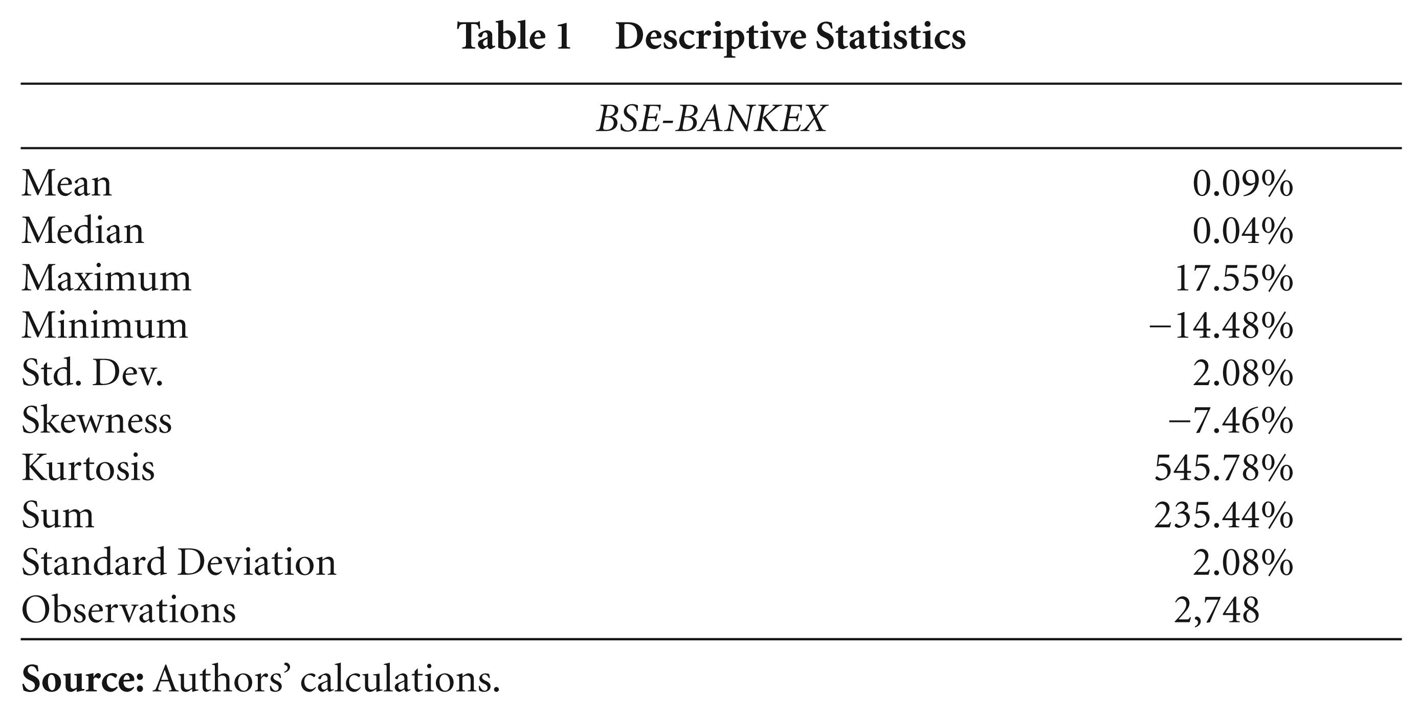
The empirical results found in this article are as follows. A time series is said to follow a normal distribution when the kurtosis and skewness are exactly equal to zero. The descriptive statistics results, as shown in Table 1, inform that BSE-BANKEX does not follow a normal distribution.

Table 1
Descriptive Statistics

BSE-BANKEX

Mean 0.09%

Median 0.04%

Maximum 17.55%

Minimum −14.48%

Std. Dev. 2.08%

Skewness −7.46%

Kurtosis 545.78%

Sum 235.44%

Standard Deviation 2.08%

Observations 2,748

BSE-BANKEX
Mean	0.09%
Median	0.04%
Maximum	17.55%
Minimum	−14.48%
Std. Dev.	2.08%
Skewness	−7.46%
Kurtosis	545.78%
Sum	235.44%
Standard Deviation	2.08%
Observations	2,748

Source: Authors’ calculations.

Stationarity is checked for the BSE-BANKEX return series with unit root tests such as the ADF and PP tests.

The results in Table 2, of the unit root test show the rejection of the null hypothesis and imply that the return series is stationary in nature.

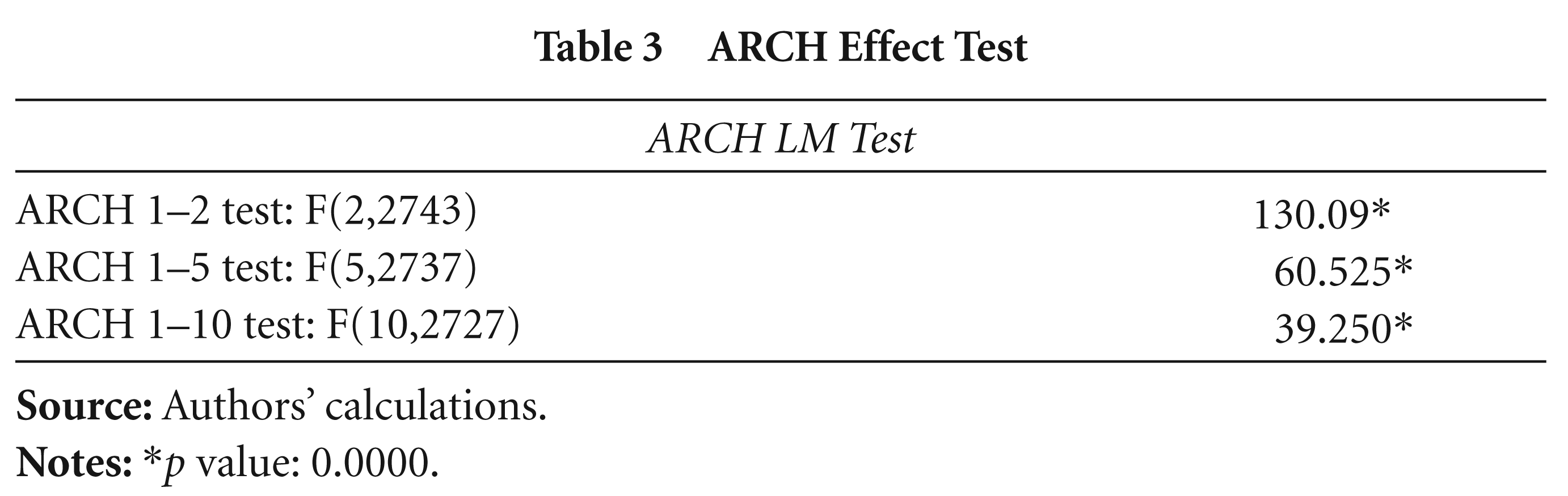
Before the estimation of the volatility and long-memory models, tests are also done to check whether Indian banking shares have an ARCH effect and long memory in their behaviour. The LM ARCH test has been done to test whether the index return has an ARCH effect. The results in Table 3, of ARCH test show significant p values, which reject the null hypothesis that there is no ARCH effect and confirm the presence of an ARCH effect.

Table 2

Augmented Dickey–Fuller (ADF) Test and Phillips–Perron (PP) Test Statistics with Lag 0

Test	Test Statistic	P Value
Augmented Dickey–Fuller	−45.85907	0.0001
Phillips–Perron	−45.55393	0.0001

Source: Authors’ calculations.

Notes: Test critical values at significance levels: 1% level is −3.432539; 5% level is −2.862393; and 10% level is −2.567269.

Table 3

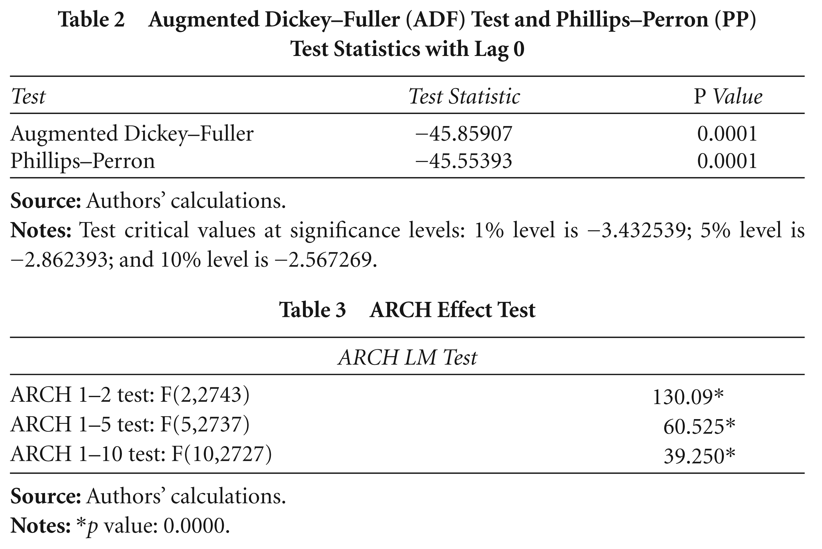
ARCH Effect Test

ARCH LM Test
ARCH 1–2 test: F(2,2743)	130.09*
ARCH 1–5 test: F(5,2737)	60.525*
ARCH 1–10 test: F(10,2727)	39.250*

Source: Authors’ calculations.

Notes: *p value: 0.0000.

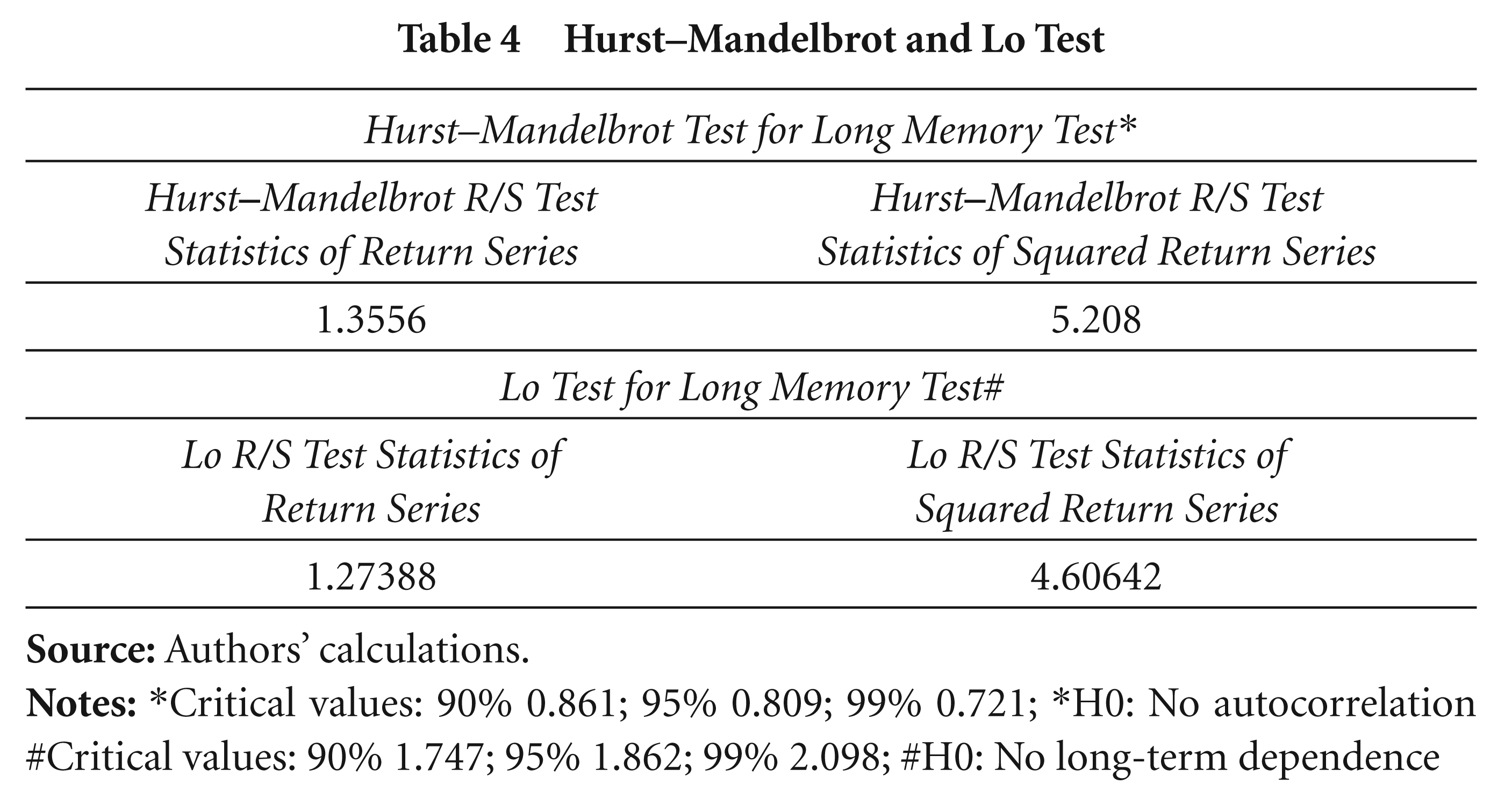
Similarly, for confirming the presence of long memory, the Hurst–Mandelbrot and Lo long-memory tests were conducted. The long-memory tests have a null hypothesis that there is no long-term dependence among the closing price returns of Indian banking share prices.

The results of the Hurst–Mandelbrot R/S test statistics reject the null hypothesis and confirm the presence of autocorrelation in the long-period return series of the closing price of Indian bank shares. However, the Lo test for long-memory does not confirm the presence of long memory in the absolute return series, but when the squared return series is taken, it confirms the presence of long memory (Table 4). Hence, it can be concluded that Indian bank shares returns have both ARCH effect and long memory.

4.1 VaR Model Estimation Results

The discussed VaR models are estimated for the return series. The models are checked for significance and found to be significant for these VaR models.

As shown in Table 5, the FIEGARCH model has the significant estimator in the case of a normal/Gaussian distribution; apart from the FIEGARCH model, the other three models are found to be significant estimators in case of a student t distribution. All the models are calculated for the ARMA (1,0) process.

Table 4
Hurst–Mandelbrot and Lo Test

Hurst–Mandelbrot Test for Long Memory Test*

Hurst – Mandelbrot R/S Test Statistics of Return Series
Hurst – Mandelbrot R/S Test Statistics of Squared Return Series

1.3556
5.208

Lo Test for Long Memory Test#

Lo R/S Test Statistics of Return Series
Lo R/S Test Statistics of Squared Return Series

1.27388 4.60642

Source: Authors’ calculations.

Notes: *Critical values: 90% 0.861; 95% 0.809; 99% 0.721; *H0: No autocorrelation #Critical values: 90% 1.747; 95% 1.862; 99% 2.098; #H0: No long-term dependence

Table 5

Estimated Statistics

	APARCH	FIEGARCH	HYGARCH	Risk Metrics
ARCH(α)	0.089132(0.0000)	−0.832638(0.0000)	0.289436(0.0000)	0.060000
GARCH(β)	0.903721(0.0000)	0.945612(0.0000)	0.684226(0.0000)	0.940000
EGARCH(θ₁)		−0.067990(0.0011)
EGARCH(θ₂)		0.385820(0.0000)
d-Figarch		0.651714(0.0000)	0.505491(0.0000)
APARCH(γ)	0.370984(0.0000)
APARCH(δ)	1.334460(0.0000)
HY (φ)			0.036939(0.0592)

Source: Authors’ calculations.

Notes: α = ARCH coefficients; β= GARCH coefficients; θ₁ = sign effect of the FIEGARCH; θ₂ = magnitude effect of the FIEGARCH; d-Figarch = long-memory coefficient; γ = asymmetry coefficients of the APARCH; δ = standard deviation of the FIAPARCH; which is δ in equations; HYφ = log(α) if the HYGARCH is used, zero otherwise.

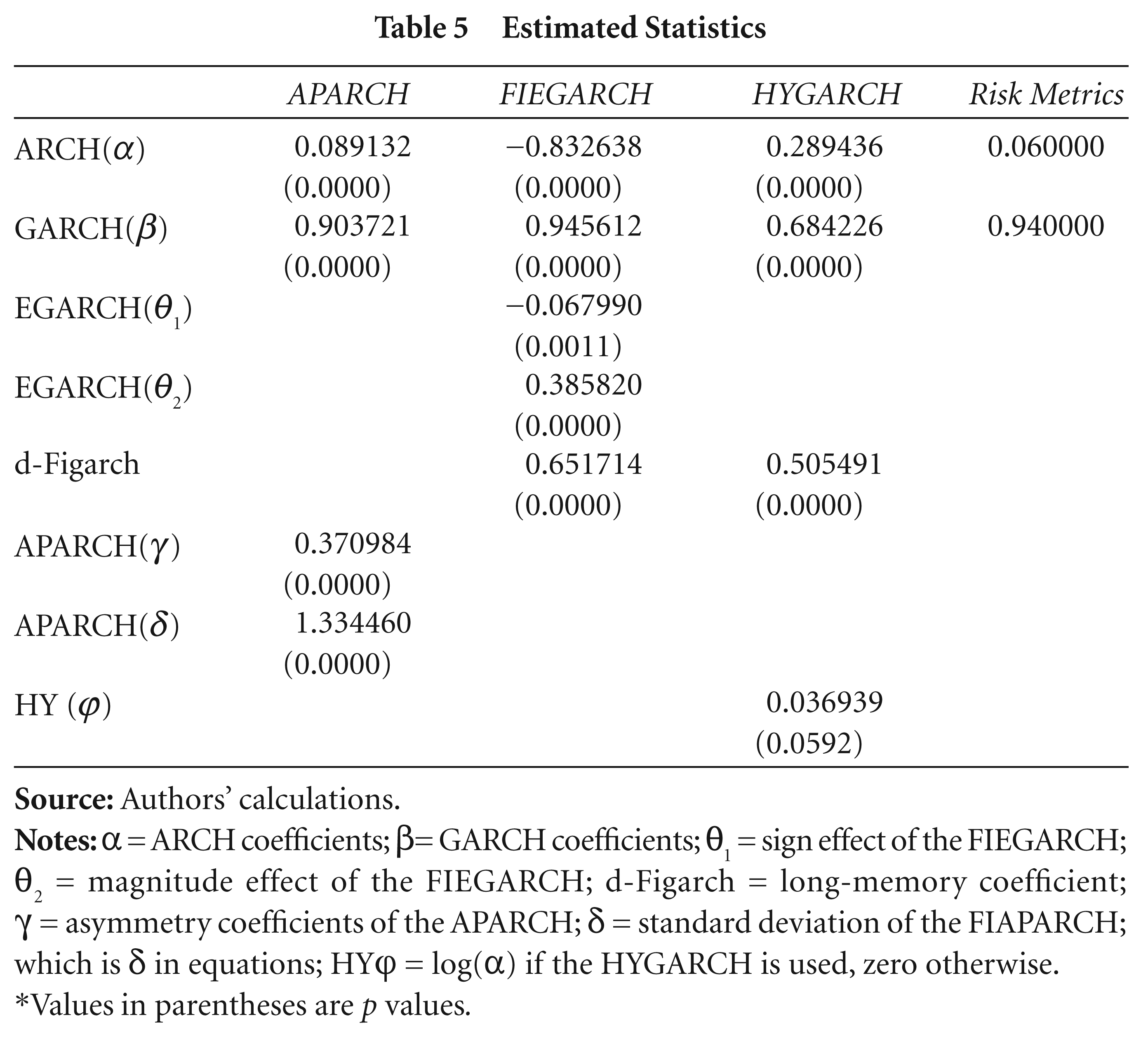
*Values in parentheses are p values.

4.2 In-sample VaR Backtesting

The Kupiec LRT and dynamic quantile test methodologies were used for backtesting each model. The models were backtested separately in considering their success and failure rate statistics.

4.2.1 The Kupiec LR test

The results arrived by the Kupiec LR test are checked for the success rate, failure rate and expected shortfall (ESF1 and ESF2) values for all the models. The Kupiec LRT statistics of the models are compared with the p value to check whether it is too large in comparison to the p values. The closeness of the LR statistics and the p values show a better estimation of the model. The ESF1 is defined as the excess value of the losses over the VaR, while the ESF2 is the degree to which events in the tail distribution exceeds the VaR. This variation in degree is calculated by the average multiple of those outcomes to their corresponding VaR measures (Hendricks, 1996).

The results arrived by the Kupiec LRT show that both asymmetries and long memory play a significant role in VaR calculations and its forecast. The models vary in their results across the short positions and long positions, but the results indicate that largely the APARCH model is best suited for both the short and long positions. The HYGARCH model follows the APARCH model in providing results for the Kupiec LR test (Refer to Appendix I for detailed results of the Kupiec LR Test for various models.)

4.2.2 Dynamic Quantile Test of Engle and Manganelli

This test is used to check VaR results by using a binary variable, one when it violates the VaR and zero when it does not violate the VaR. The test is done with the assumption that the sequence of VaR violations is not serially correlated.

The dynamic quantile test results show that the null hypothesis is mostly accepted for the models, which indicates that both the asymmetries and long-memory models play a significant role in VaR calculation and its forecast. The results vary for the short positions and long positions among the models, and the long-memory models show a better result for both short and long positions in the dynamic quantile test. (Refer to Appendix II for detailed results of the dynamic quantile test for various models.)

4.3 Forecast Evaluation Measures

Forecast evaluation is done with the help of MAE and RMSE statistics and the model with a low error statistics is preferred for forecast.

The low error statistics of the models show a good VaR forecasting capacity. There is a slight difference in the estimated error statistics for all the selected models. To conclude, the long-memory HYGARCH model yields a slightly better result than the other models. (See Table 1 in Appendix III.)

The forecast returns for all the models are shown in comparison to the actual returns. The results indicate that the models used approximately forecast the true return series, except for the FIEGARCH that is conservative in forecasting and the HYGARCH model that forecasts the return series a little than the other models used here. All the models forecast the VaR at both the 0.95 per cent and 0.05 per cent confidence levels. (See Figures 1–4 in Appendix IV.)

The HYGARCH model has the least variance forecast in the estimated model compared to the other models. The forecast at both the 0.95 per cent and 0.05 per cent confidence levels is also good in this model as it has a perfect balance between the level of confidence intervals.

The forecast result of the mean return series compares the forecast return of the different models applied with the actual observed return of the daily BSE-BANKEX and shows that the HYGARCH model has a better forecast capacity than the other models used. The RiskMetrics and APARCH models follow the HYGARCH model in predicting the return series. (See Table 2 in Appendix III.)

5. THE GFC AND VAR LIMITATIONS

The VaR method is based on many complicated assumptions and the use of this VaR model centres around the probability concept. This probable estimation may not always provide the actual forecast result if the model and its assumptions are not properly selected. Among many factors such as faulty credit ratings of loans, secured subprime mortgages from Fannie Mae and Freddie Mac and highly priced mortgage-backed securities, the use of the VaR technique by banks is also one of the factors responsible for the GFC. Most of the financial theories are based on the concept an efficient market hypothesis and a normal distribution, and the simple VaR model is also based on a normal distribution that has a chance of failure. To solve this problem, advanced VaR models have been proposed. However, the problem lies with the selection of the model. The accuracy of the VaR model can be ensured by regularly backtesting the model and evaluating the results by efficient users. Proper caution and testing of alternative VaR models need to be done.

6. CONCLUSION

This study had analysed various VaR models and compared the estimated results. It gives an overview of both the asymmetry and long-memory models, and then substantiates them through advanced tests. The study is unique in the sense that it takes the sectoral index BANKEX as the return series for analysis, whereas either the BSE-Sensex or the NSE-Nifty return series are usually studied in India. The current study investigates and confirms the presence of asymmetry and long-memory characteristics in the BSE-BANKEX return series. In spite of varied results from the different VaR models, the HYGARCH model outperforms all the models in estimating the VaR and forecasting the return series. However, the other models such as the APARCH, FIEGARCH and RiskMetrics are also important tools for VaR calculation of bank shares in India.

This study will add to the existing literature of VaR models and their backtesting for Indian case studies. Its findings may throw light on sector-specific VaR calculations and help researchers study different sectors separately to have a better view of the VaR.

Footnotes

APPENDICES

Notes

References

Aloy

, Dufrenot

, Tong

C. L.

, & Feissolle

A. P.

(2012). A smooth transition long-memory model, Working Paper number 40, Aix-Marseille University, Provence.

Assaf

(2002). An examination of long memory in the Canadian/US dollar exchange rate returns and volatility. Finance Proceedings from ACAS’02: The Annual Conference of the Administrative Sciences Association of Canada Finance Division, Winnipeg, Manitoba, 23(1), 1–8.

Berkowitz

, & Obrien

(2002). How accurate are value-at-risk models at commercial banks? The Journal of Finance, 57(3), 1093–1111.

Blanco

, & Oks

(2004). Backtesting VaR models: Quantitative and qualitative tests. The Risk Desk, IV(1).

Bollerslev

, & Mikkelsen

H. O.

(1996). Modelling and pricing long memory in stock market volatility. Journal of Econometrics, 73(1), 151–84.

Bucevska

(2013). An empirical evaluation of GARCH models in value-at-risk estimation: Evidence from the Macedonian stock exchange. Business Systems Research, 4(1), 49–64.

Davidson

(2004). Moment and memory properties of linear conditional heteroscedasticity models and a new model. Journal of Business & Economic Statistics, 22(1), 16–29.

Ding

, Granger

C. W. J.

, & Engle

R. F.

(1993). A long memory property of stock market returns and a new model. Journal of Empirical Finance, 1(1), 83–106.

Dutta

, & Bhattacharya

(2008). A bootstrapped historical simulation value at risk approach to S&P CNX Nifty. The National Conference on Money and Banking, IGIDR, Mumbai, India.

10.

Engle

R. F.

(1982). Autoregressive conditional heteroscedasticity with estimates of the variance of United Kingdom inflation. Econometrica, 50(4), 987–1007.

11.

Floros

, Jaffry

, & Lima

G. V.

(2007). Long memory in the Portuguese stock market. Studies in Economics and Finance, 24(3), 220–32.

12.

Gourieroux

, Laurent

J. P.

, & Scaillet

(2000). Sensitivity analysis of values at risk. Journal of Empirical Finance, 7(3), 225–45.

13.

Hendricks

(1996). Evaluation of value-at-risk models using historical data. Federal Reserve Bank of New York: Economic Policy Review.

14.

K. Y.

, Shi

, & Zhang

(2013). How does news sentiment impact asset volatility? Evidence from long memory and regime-switching approaches. North American Journal of Economics and Finance, 26, 436–56.

15.

Huang

A. Y.

, & Tseng

T. W.

(2009). Forecast of value at risk for equity indices: an analysis from developed and emerging markets. The Journal of Risk Finance, 10(4), 393–409.

16.

Kupiec

(1995). Techniques for verifying the accuracy of risk measurement models. Journal of Derivatives, 2(3), 73–84.

17.

A. W.

(1991). Long-term memory in stock market prices. Econometrica, 59(5), 1279–1313.

18.

Manap

T. A. A.

, & Kassim

S. H.

(2011). Long memory properties and asymmetric effects of emerging equity market: Evidence from Malaysia. The Journal of Risk Finance, 12(5), 356–70.

19.

Mandelbrot

(1972). A statistical methodology for non-periodic cycles: From the covariance to R/s analysis. Annals of Economic and Social Measurement, 1(3), 259–90.

20.

McMillan

, & Thupayagale

(2010). Evaluating stock index return value-at-risk estimates in South Africa: Comparative evidence for symmetric, asymmetric and long memory GARCH models. Journal of Emerging Market Finance, 9(3), 325–45.

21.

Morgan

J. P.

(1996). Riskmetrics technical document. New York: J. P. Morgan.

22.

Nelson

D. B.

(1991). Conditional heteroscedasticity in asset returns: A new approach. Econometrica, 59, 349–70.

23.

Poon

S. H.

(2005). Linear and Nonlinear Long Memory Models. In Poon

S. H.

(Ed.), A practical guide to forecasting financial market volatility (pp. 45–58). Chichester: John Wiley & Sons Ltd.

24.

Sarma

, Thomas

, & Shah

(2003). Selection of value-at-risk models. Journal of Forecasting, 22(4), 337–58.

25.

Varma

J. R.

(1999). Value at risk models in the Indian stock market, Working Paper 99–07. IIM, Ahmedabad.

26.

Wang

C. S.

, Bauwens

W. L.

, & Hsiao

(2013). Forecasting a long memory process subject to structural breaks. Journal of Econometrics, 177(2), 171–84.

Hurst–Mandelbrot Test for Long Memory Test*
Hurst – Mandelbrot R/S Test Statistics of Return Series	Hurst – Mandelbrot R/S Test Statistics of Squared Return Series
1.3556	5.208
Lo Test for Long Memory Test#
Lo R/S Test Statistics of Return Series	Lo R/S Test Statistics of Squared Return Series
1.27388	4.60642

Backtesting of Value at Risk Methodology: Analysis of Banking Shares in India

Abstract

Keywords

1. INTRODUCTION

2. LITERATURE REVIEW

3. DATA AND METHODOLOGY

3.1 The LM ARCH Test

3.8.1 The Kupiec LR test

Table 1 Descriptive Statistics BSE-BANKEX Mean 0.09% Median 0.04% Maximum 17.55% Minimum −14.48% Std. Dev. 2.08% Skewness −7.46% Kurtosis 545.78% Sum 235.44% Standard Deviation 2.08% Observations 2,748

4.2.1 The Kupiec LR test

4.2.2 Dynamic Quantile Test of Engle and Manganelli

4.3 Forecast Evaluation Measures

5. THE GFC AND VAR LIMITATIONS

6. CONCLUSION

Footnotes

APPENDICES

Notes

References

Table 1
Descriptive Statistics

BSE-BANKEX

Mean 0.09%

Median 0.04%

Maximum 17.55%

Minimum −14.48%

Std. Dev. 2.08%

Skewness −7.46%

Kurtosis 545.78%

Sum 235.44%

Standard Deviation 2.08%

Observations 2,748