
Abstract
This article attempts to determine the method of volatility estimation that prices the CNX Nifty Index options closest to the theoretical price as computed by the Black–Scholes (1973) model. Volatility has been estimated using simple variance, implied volatility, volatility index and the asymmetrical exponential generalised auto-regressive conditional heteroskedasticity (EGARCH) (1,1) model with generalised error distribution innovations. The trend in mispricing has been studied using error estimates and non-parametric tests. Our findings indicate significant mispricing in CNX Nifty Index options. The results of our study will have major implications for investors who use options as part of their portfolios and corporates who use them for risk hedging. Our study is important, as there are only a few studies that examine the pricing efficiency of options with a focus on volatility modelling. Also, our study spans a longer time period than the previous studies.
Keywords
Introduction
Financial volatility refers to the intensity of fluctuations in the expected return on an investment or pricing of a financial asset due to market uncertainties. Hence, volatility modelling is imperative to financial market investors; such projections allow investors to adjust their trading strategies in anticipation of impending financial market movements (Tung & Quek, 2011). In addition to being an important precursor to the management of risk, the estimation of volatility also forms a basis for arbitraging on volatility in future. A large part of risk management involves measuring potential future losses of a portfolio of assets, and in order to measure these potential losses, estimates must be made of future volatilities and correlations (Reider, 2009).
In the case of options trading, volatility estimation is an important decision criterion. While adopting model-based approaches to options pricing, this criterion assumes primary importance, as it is the one input that is not directly observable from the market, and therefore needs to be estimated.
Of the various methods available to researchers for the estimation of volatility, the most appropriate method is the one which, when substituted into a pricing model, yields a theoretical price that is closest to the observed market price. In other words, while all other inputs to the option pricing model are kept invariant, this particular measure of volatility results in the best pricing efficiency for the pricing model.
In the present study, an attempt has been made to evaluate alternate volatility measures that yield the highest pricing efficiency when options price is measured using the Black–Scholes (BS) model. The contract under investigation is the CNX Nifty Index Options, traded on India’s National Stock Exchange (NSE). The alternate measures of volatility that we examine are: traditional volatility estimators, which are generally estimated standard deviation of returns; implied volatility (IV) and conditional volatility models. The sample study period spans 10 years, from January 2003 to December 2012.
Literature Review
Since the time Fisher Black and Myron Scholes promulgated their celebrated model in 1973, which was modified by Robert Merton in the same year, there has been a plethora of studies, especially in the more established Western markets. The studies are largely in the area of volatility modelling and pricing efficiency. There has been a considerable overlap, too, in most of the papers, since these concepts are intertwined.
From the immense literature available, four methods of volatility estimation appear to be most prevalent—largely pertaining to adjudging pricing efficiency in options markets—and these are reviewed as follows.
Simple Variance
Simple variance is the simplest method of computation of historical volatility (HV). It is regarded as the most naive method for volatility estimation. The literature reviewed has been studied under two sub-headings.
Historical volatility good predictor of future volatility/historical volatility better than other methods of volatility estimation/inconclusive evidence. HV has been used in the BS model considerably, but with developments in financial theory, the very concept of HV has taken a backseat in the minds of researchers. This is basically on account of its simplistic assumptions that volatility can be forecast from past prices. However, in newer and less mature markets, HV does find its place, since the market participants do not use other complicated methods of estimating volatility. There are only a handful of studies that report HV as a good predictor of future realised volatility.
In Toronto, Doidge and Wei (1998) found HV a better measure than IV, contrary to results in other markets. Lung and Marshall (2002) find inconclusive evidence between the relationships of mispricing with volatility. Ederington and Guan (2006) sought a simple volatility estimate, which could prove to be a good estimator for future volatility. They deduced that log-adjusted historical deviation performed favourably, almost at par with the generalised auto-regressive conditional heteroskedasticity (GARCH) model. Sehgal and Vijayakumar (2009) tested pricing efficiency using both HV and weighted IV and testified that the market used HV estimates in option valuation in India.
Historical volatility poor predictor of future volatility. Cohen, Black and Scholes (1972) used the BS model and reported that using HV in the model caused overpricing in options on high variance stocks and underprice options on low variance stocks. Brown and Shevlin (1983) used both HV and weighted implied standard deviation (WISD) to price options and deduced that using HV underpriced the model. Cotner and Horrell (1989) reported that the pattern of mispricing using HV was similar to that when IV was used; however, with IV, there were smaller errors. Evans and McMillan (2007) evaluated several models of estimation of volatility and reported that HV performed worst.
It can be inferred from the above discussion that there are fewer studies that prove the superiority of HV as a forecaster of volatility. However, this method has been extensively used in derivative markets that are new, since market participants may not be aware of the more sophisticated techniques of volatility modelling.
Implied Volatility (IV)
IV has attracted a great deal of academic research. Specifically, the information content of IV regarding future volatility and the existence of a volatility ‘smile’ has been the subject of several research works. Interestingly, the literature is divided on the performance of IV. They are discussed as follows.
IV good predictor of future volatility/better than other methods of volatility estimation/Inconclusive evidence. Chiras and Manaster (1978) used the BS model and found that implied variance was better than one derived from historical stock price data. Brown and Shevlin (1983) compared HV and WISD to price options and deduced that using the WISD greatly improved performance of the model. Although Cotner and Horrell (1989) reported that the pattern of mispricing using HV was similar to that when IV was used, they reported that IV definitely gave smaller errors. Christensen and Prabhala (1998) used non-overlapping data series in S&P 100 Index Options and reported that IV outperforms past volatility. Hansen (2001) studied the Danish index and reported that after controlling for measurement errors, call option prices contained information about future realised volatility more so, compared to HV. Taylor, Yadav & Zhang (2007) studied a large number of US firms and deduced that at the money (ATM) implied that volatility outperforms other methods of volatility estimation for majority of the firms.
Yu, Lui and Wang (2008) suggested that IV was superior to HV and GARCH-type volatility forecast in predicting future volatility in both the over-the-counter (OTC) and exchange markets. Panda, Swain & Malhotra (2008) investigated the information content of IV forecast in Indian markets, following the procedure proposed by Christensen and Prabhala (1998). The study reported the superiority of IV forecast over past-realised volatility. Although IV was efficient, it was still a somewhat biased estimator. Kumar (2008) reported that IV has information on future volatility and is a better estimator than HV. The study concluded that IV derived from call options had better predictive ability than put options IV. Li and Yang (2009) studied the Australian market and found call IV to be an unbiased predictor of future volatility. Dixit, Yadav and Jain (2010) found in their research that IV in the Indian market is mean-reverting, but investors do not use the term structure approach to price option contracts.
IV a poor predictor of future volatility/a biased predictor. Day and Lewis (1992) stated that IV was a poor predictor of future realised volatility. They found similar results related to GARCH and exponential GARCH (EGARCH) models, although the presence of ARCH elements did improve predictability. Lamoureux and Lastrapes (1993) examined IV and demonstrated that it is biased and inefficient, and that usage of the GARCH models gave better results. However, they used overlapping data for their study. Canina and Figlewski (1993) studied the US markets and reported that IV has poor informational content on future volatility. Claessen and Mittnik (2002) examined alternate strategies for predicting stock market volatility using the BS Model and found that IV tended to overstate the actual volatility of DAX index returns.
Volatility Index (VIX)
Brenner and Galai (1989) suggested construction of a volatility index (VIX) and derivatives based on the same, although the idea had existed since 1973. The Chicago Board Options Exchange (CBOE) introduced the VIX in 1993 and since then it has been widely recognised. However, the literature connecting the VIX and option pricing is quite scant.
VIX is a model-free estimate of IV; therefore, it does not suffer from the limitations of assumptions of the model. Moraux, Navatte & Villa (1999) examined the forecasting performance of the French VIX and reported that it is a good predictor of future volatility.
Giot (2005) showed that there is a negative and statistically significant relationship between returns of the stock and IV, using data from CBOE. Also, the study reported that negative changes in volatility caused higher changes in the VIX, compared to positive changes. Taylor et al. (2007) contradicted these results and opined that historical models of conditional variances outperformed the model-free methods of estimation of volatility for more than one-third of the firms studied.
The Indian VIX was launched in November 2007 on the basis of CBOE methodology. Banerjee and Kumar (2011) compared the performance of the VIX and the GARCH model and deduced that forecast error is lowest for the VIX, even compared to the GARCH. Singh and Ahmad (2011a) studied the Indian market and inferred that IV from the BS model outperformed both VIX and GARCH estimates. Kanniainen, Binghuan & Yang (2014) used the VIX and the S&P 500 Index returns for option valuation and deduced that this joint method clearly outperformed the method where only stock returns were used.
It can be summarised from the above that although the forecasting ability of the VIX has been the subject of study in many studies, its usage in option valuation as an input for volatility seems to be limited.
GARCH Family of Models
Engle (1982) introduced the ARCH model and changed the landscape of volatility modelling and, thus, financial markets. Nelson (1991) propagated the EGARCH, which is better suited for stock markets, since stock returns are more affected by bad news than good news. Since then, there has been a plethora of ARCH type of models, both symmetric and non-symmetric. Thereupon, a number of studies have been taken up using the GARCH family of models. A brief review pertinent to the present study is presented below.
Day and Lewis (1992) observed that the GARCH and EGARCH models had incremental information compared to the IV for within the sample data. Lamoureux and Lastrapes (1993) opined that the simple GARCH (1, 1) model subsumes greater information than IV based on the data for ten US firms for two years.
Franses and Dijk (1996) examined the predictability of standard GARCH models and asymmetric models, and indicated that the Quadratic GARCH model gave superior forecasts. Doidge and Wei (1998) studied Canadian markets and reported that EGARCH was outperformed by the GARCH model by a slight margin. Varma (1999) reported that the GARCH model failed miserably in the Indian exchange rate market, which could be attributed to the exclusion of kurtosis from the computation in the model. McMillan, Speight & Apgwilym (2000) disagreed with many previous studies and deduced that the GARCH family of models did not provide superior results compared to the random walk model. Pandey (2005) indicated that while conditional volatility models performed well in estimating volatility for the past in terms of bias, extreme value estimators based on observed trading range perform well on efficiency criteria. Engle (2001) examined the application of the GARCH (1, 1) model in financial econometrics and suggested various extensions like GARCH (p, q), usage of asymmetric models and, finally, incorporating multivariate modelling.
Banerjee and Sarkar (2006) indicated that the Indian stock market depicted volatility clustering and demonstrated that asymmetric models were a better fit, compared to simple GARCH models in India. Evans and McMillan (2007) evaluated several volatility models for 33 economies and deduced that GARCH-type models performed well, especially those that account for a leverage affect. Singh and Ahmad (2011b) compared the alternate volatility models using the BS model. They suggested the presence of GARCH elements improved the pricing accuracy of the model. Singh and Ahmad (2011a) deduced that IV outperforms benchmark GARCH volatility and VIX models in most moneyness–maturity groups.
It is evident from the above discussion that many variations of the theme under study have been taken up in the past. All the above studies, in the context of Indian market, largely differ on account of the methodologies adopted; therefore, a conclusion regarding the pricing efficiency based on different volatility estimates may not be appropriate. Also, for most of these, the study period is small due to the newness of the market in India. This article attempts to fill this gap by taking up a 10-year period to study the market efficiency represented by CNX Nifty Index Options. Pricing accuracy using the BS model will also denote the best estimate of a volatility model.
Data and Methodology
Data
Our study focuses on CNX Nifty Index Call Options. The main objective of the study is to determine which method of volatility estimation yields a theoretical price of CNX Nifty Index Options closest to the observed price. The sample study period spans 10 years, from January 2003 to December 2012. Wherever deemed necessary, the study period has been divided into sub-periods to discern a meaningful pattern of efficiency/inefficiency. These sub-periods are: 2003–07, 2008–12 and 2010–12 (the period for which VIX is available).
The data for the present study consist of three sets:
Data related to options contracts like transaction date, expiry date, daily closing price and number of contracts traded. Data pertaining to the daily spot index like the price of the underlying and dividend yield. The risk-free interest rate, for which we have used the 30-day Mumbai Inter-Bank Offer Rate (along the lines of Kumar, 2008; Tiwari & Saurabha, 2008).
All the above-mentioned datasets have been taken from the official website of NSE. 1 The dividend yield and risk-free interest rate have been continuously compounded. At NSE’s index options segments, the volumes are concentrated around near-term expiry; therefore, the same have been chosen for the study.
Data Screening Procedure
A series of steps have been taken to eliminate data that may introduce potential biases in the study. When options are not traded, the price is the theoretical one. The contract for which there has been no trading has been taken off from the sample. This is similar to the approach of Berg, Brevik & Saettem (1996) and Sehgal and Vijayakumar (2009). Observations made on the expiry day have been excluded from the sample, primarily on account of increased trading volume around the expiry day (Vipul, 2005).
Observations remaining after applying these data filters are checked for lower boundary conditions (LBC) (Bates, 1996). All those contracts where the LBC has been violated are removed from the sample. After this screening process, there are 45,657 observations for the study.
The Black–Scholes (BS) Model
For the purpose of our study, we record a mispricing signal when there is a difference between the observed price and the theoretical price of the Nifty Index Option as determined by the BS model (1973).
Dividend Adjustment
Dividends cause stock prices to decrease on the ex-dividend date by the amount of the dividend payment (Hull & Basu, 2010). The dividend adjustment procedure given by Merton requires substituting the value S0' for S0 in the BS model, where S0' = S0e–dT, where d is the continuously compounded annual dividend yield, T is the time to expiry of the option in years, and S0 is the price of the underlying in the spot market.
Volatility Models
As can be seen from the above, volatility is the only unobservable input in the BS model (1973). In the present study, volatility has been estimated by the methods discussed:
Simple Variance Estimate of Historical Volatility
The HV of an asset is measured as the annualised standard deviation of the returns on the asset over some historical period of time. The look-back window has been taken as 30 days, since the options have around 30-day expiry (Hull & Basu, 2010).
The standard deviation can be estimated using:

where,
n is the number of observations
ui is the expected stock return
The daily volatility so calculated is converted into an annualised measure using the following:
The present study utilises trading days for annualising volatility following Kakati (2006), Mitra (2008) and Kumar (2008).
Implied Volatility–Black–Scholes
IV is widely interpreted as the market expectation of the underlying stock’s return volatility over the remaining life of the option (Wang, Yourougou & Wang, 2012). Unlike HV, it is forward-looking in nature. At India’s NSE, option contracts expire on the last Thursday of every month. In the present study, the nearest-to-the-money (NTM) contract is identified as Friday, that is, the day on which a fresh contract is introduced. The IV is computed for the same and has been used as a predictor for volatility for the remaining life of the option. The ‘Goal Seek’ function of Microsoft Excel is used to calculate the IV in the present study.
Implied Volatility–Volatility Index (VIX)
To calculate IV, an option valuation model like the BS is needed along with its inputs. As a result, the IV forecasting is as robust as the specifications of the model and the estimation of the model variables. Using an IV index like the VIX may mitigate the problem. The VIX is a model-free measure of a market’s expectation of volatility over the near term. It is expressed as the annualised percentage of volatility for the next 30 calendar days. The data for the VIX calculated for 30 days in case of Nifty 50 Index Option contracts are available from March 2009 at the NSE. Therefore, for the last three years of the sample period (2010–12), the VIX has been used in the BS model to arrive at the theoretical call option prices for the Nifty Index Options.
Exponential Generalised Auto-regressive Conditional Heteroskedasticity (EGARCH) with Generalised Error Distribution (GED)
The most important stylised facts about volatility are known as volatility clustering, leptokurtosis and the leverage effect (Kun, 2011). To capture these, conditional volatility models are used. According to a comprehensive literature review by Poon and Granger (2003), EGARCH and other asymmetric models perform better in many studies. In the Indian context, Banerjee and Sarkar (2006) and Dutta (2010) confirm the presence of the leverage effect and suggest that asymmetric models beat the GARCH model.
The financial return series is known to have excess kurtosis, so the generalised error distribution (GED) is deemed to be appropriate for the study. The GED as proposed by Nelson (1991) is a symmetric distribution, which can be both leptokurtic and platykurtic.
This use of the model is validated using statistical methods in the present study. The applicability of the statistical tools used is established as follows:
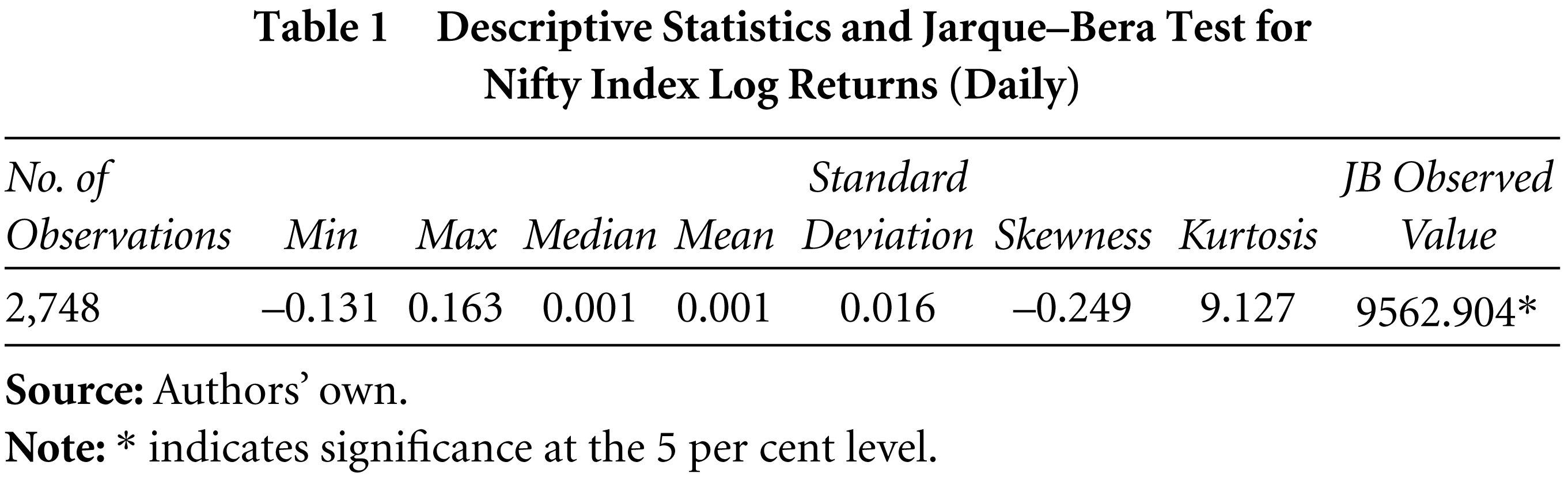
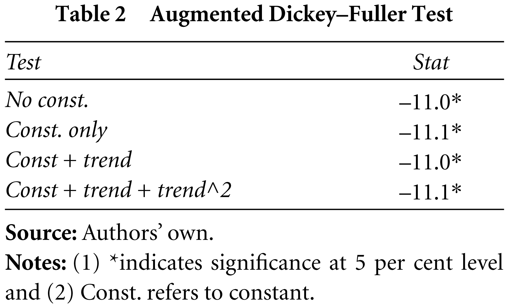
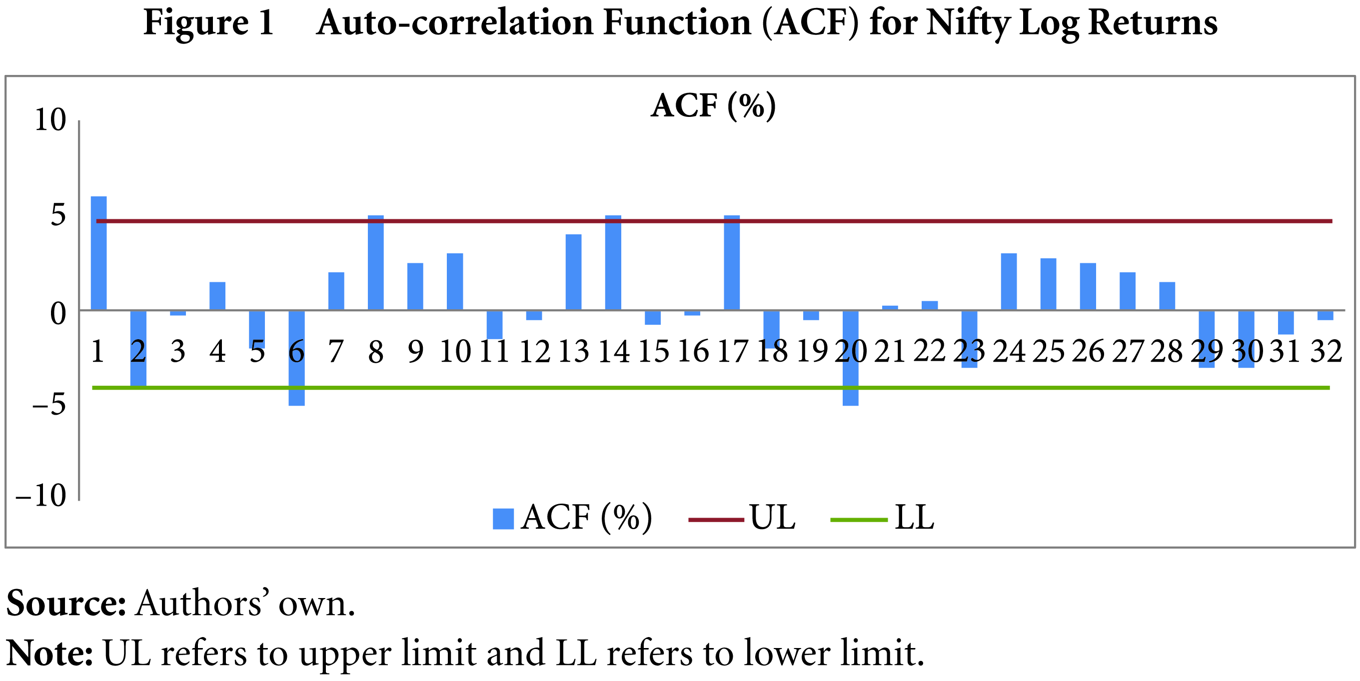
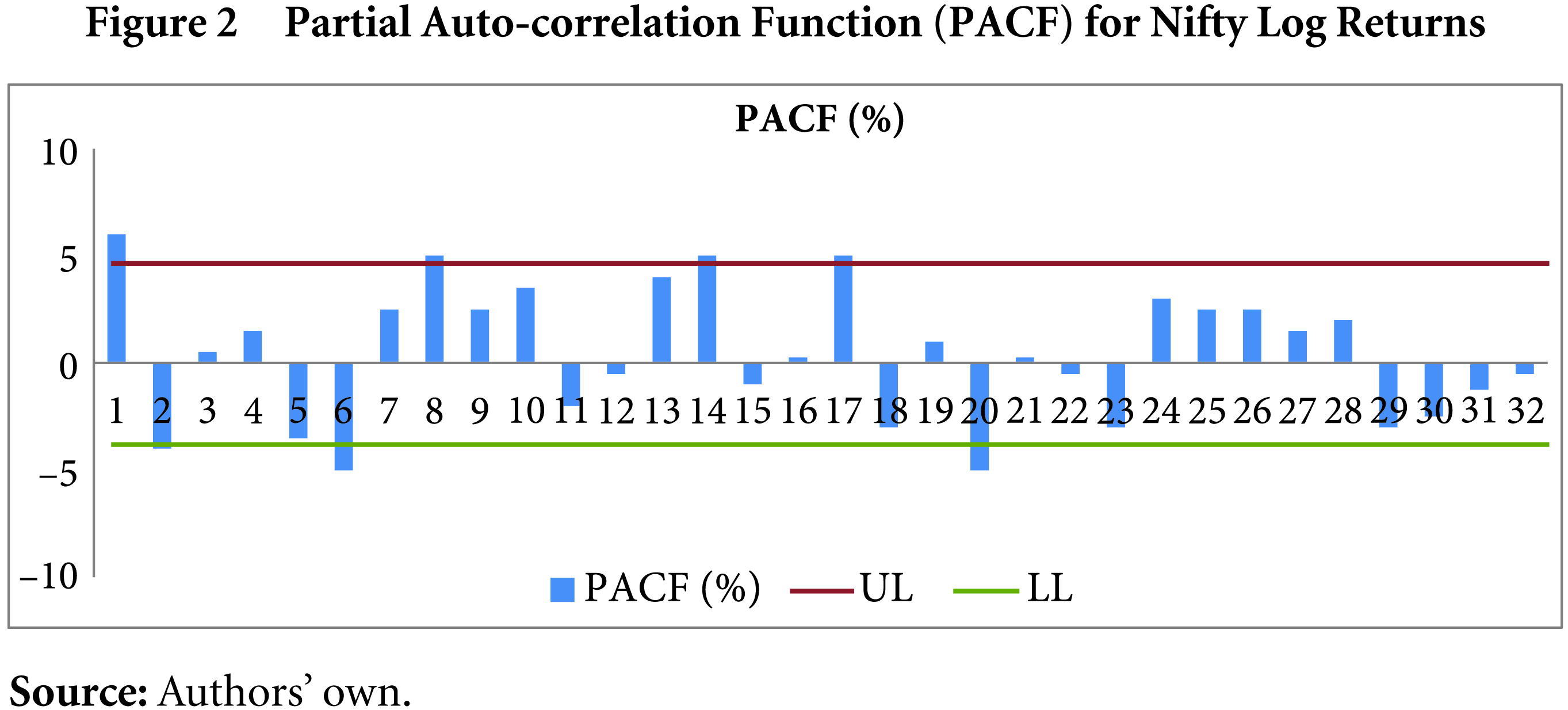
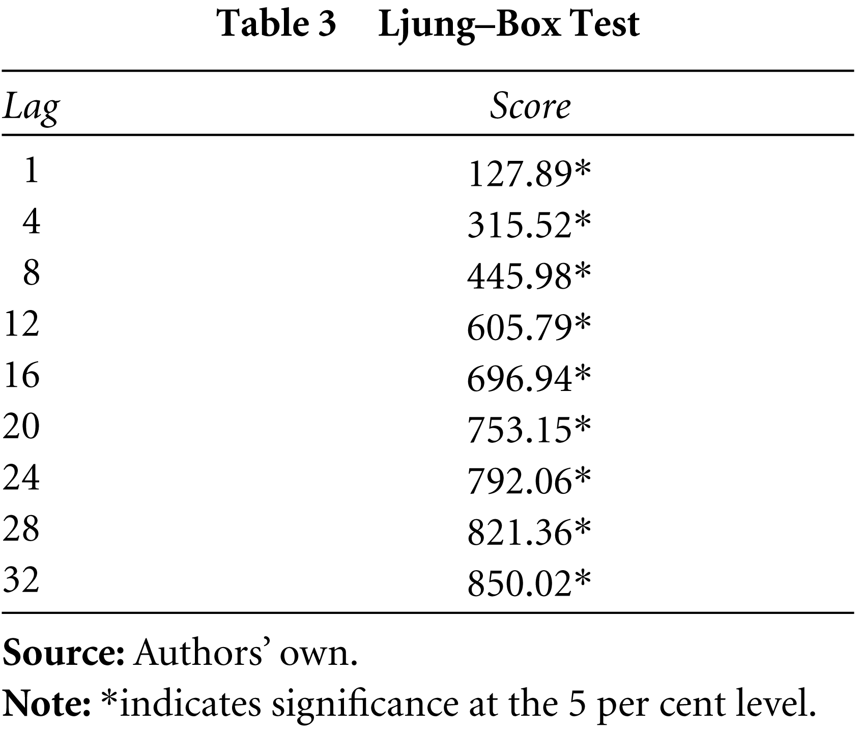
The ARCH models assume normality of the distribution. To test this, the skewness, kurtosis and Jarque–Bera (JB) test is used (results are in Table 1). The distribution is approximately symmetrical as denoted by the skewness. The excess kurtosis depicts severe departure from normality. The JB statistic also rejects the null hypothesis that the samples are drawn from a normal distribution at the 5 per cent significance level. The time varying nature of volatility can be tested using unit root tests. In the present study, the Augmented Dickey Fuller Test (ADF) is used to verify stationarity in the time series. The results (Table 2) indicate that the series is stationary. Volatility clustering is caused by autocorrelation in the time series, which can be observed from the auto-correlation function (ACF) and the partial ACF (PACF) in Figures 1 and 2. Serial auto-correlation can be seen up to 32 lags, which can also be verified statistically by using Ljung–Box statistics at specified lags (Table 3).
Descriptive Statistics and Jarque–Bera Test for Nifty Index Log Returns (Daily)
Descriptive Statistics and Jarque–Bera Test for Nifty Index Log Returns (Daily)
Augmented Dickey–Fuller Test
Ljung–Box Test
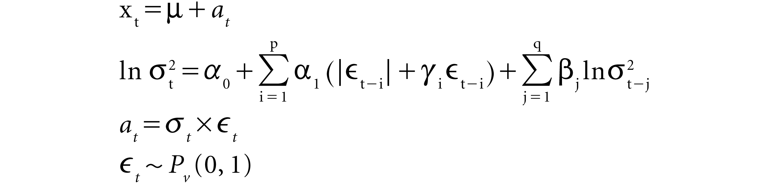
It is evident from the above that EGARCH cannot be used under the assumptions of a Gaussian distribution for the Nifty Index Options. The EGARCH with GED innovations is modelled in the present study. The EGARCH (GED) is specified as follows:
Where:
xt
is the time series value at time t.
μ
is the mean of GARCH model.
at
is the model’s residual at time t.
σt
is the conditional standard deviation (i.e. volatility) at time t.
P
is the order of the ARCH component model.
α0, α1, α2,…., αp
are the parameters of the ARCH component model.
q
is the order of the GARCH component model.
β1, β2, ….., βq
are the parameters of the GARCH component model.
ϵt
are the standardized residuals:
[ϵt] ∼ i. i. d
E[ϵt] = 0
Var[ϵt] = 1
Pv
is the probability distribution function for ϵt. For Generalized error distribution (GEDi)
Pv = GEDv(0, 1)
v > 1
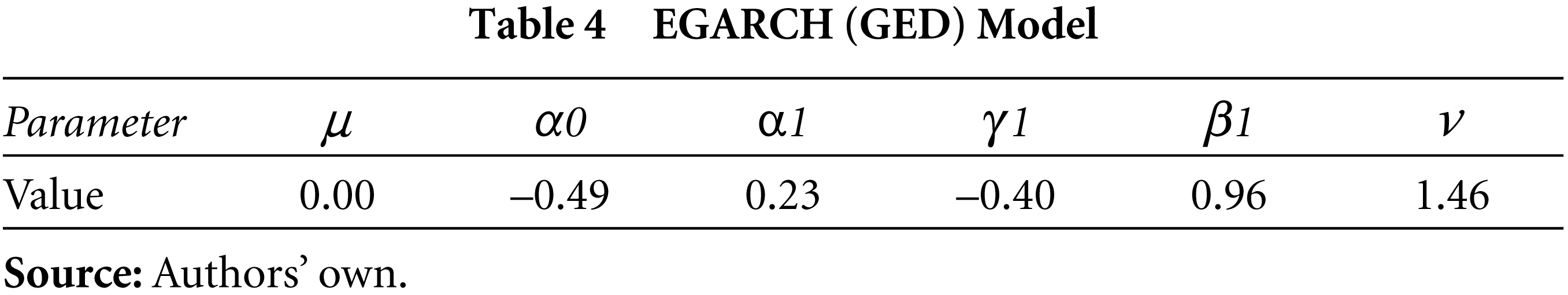
The parameters thus estimated are shown in Table 4.
EGARCH (GED) Model
In most empirical studies, error estimates are used to evaluate the performance of the competing models for forecasting. The following notations are used:
Ymod
= The theoretical model price of the option
Yobs
= Observed market price of the option
N
= Number of observations


Thus, a value closer to zero will give a good fit to a forecasting model. The MAPE measure is less sensitive to outlier distortions and allows for a direct comparison between different forecasting methods.
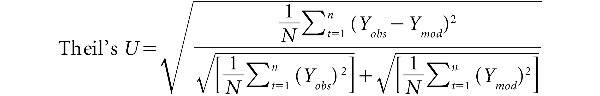
Theils’s U-statistic can be used to compare the estimated model and the benchmark model. If Thiel’s U is less than 1, the method is superior to a naive forecast. It can be described as:
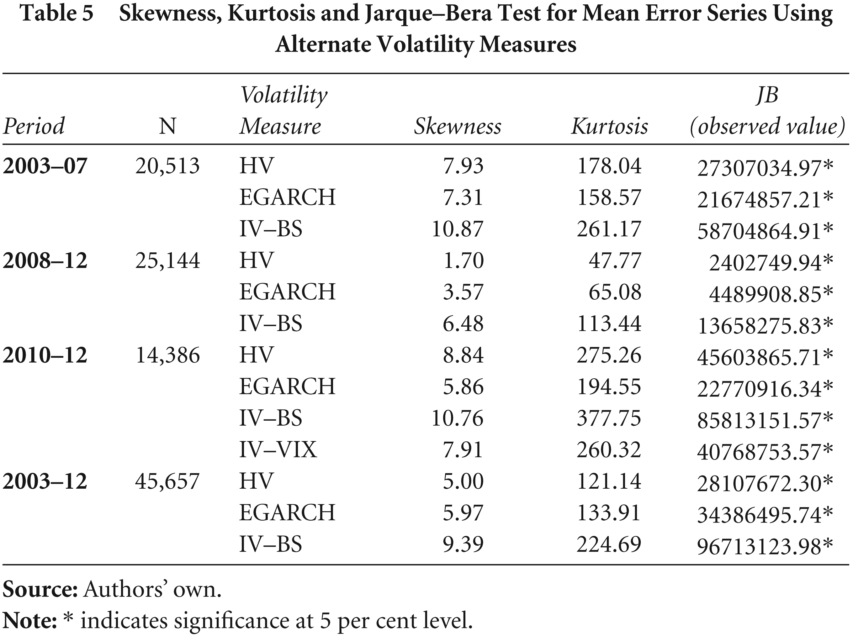
The ME series is checked for normality using the JB test. Significant departure from normality was observed for all methods of volatility, for all sub-periods (Table 5), so, non-parametric tests would be more suitable for the study.
Skewness, Kurtosis and Jarque–Bera Test for Mean Error Series Using Alternate Volatility Measures
Skewness, Kurtosis and Jarque–Bera Test for Mean Error Series Using Alternate Volatility Measures
The Wilcoxon signed rank test is used to analyse whether there is any significant difference between the market price of options and the price as calculated by applying the BS model.
The Diebold Mariano (DM) test (Diebold & Mariano, 1995) considers the model-free tests of forecast accuracy that are applicable to forecast errors that are non-Gaussian, non-zero mean, serially correlated and contemporaneously correlated. In the present study, a one-tailed test is used for comparative analysis of the competing volatility estimates.
Error Estimates Using HV and EGARCH (GED)
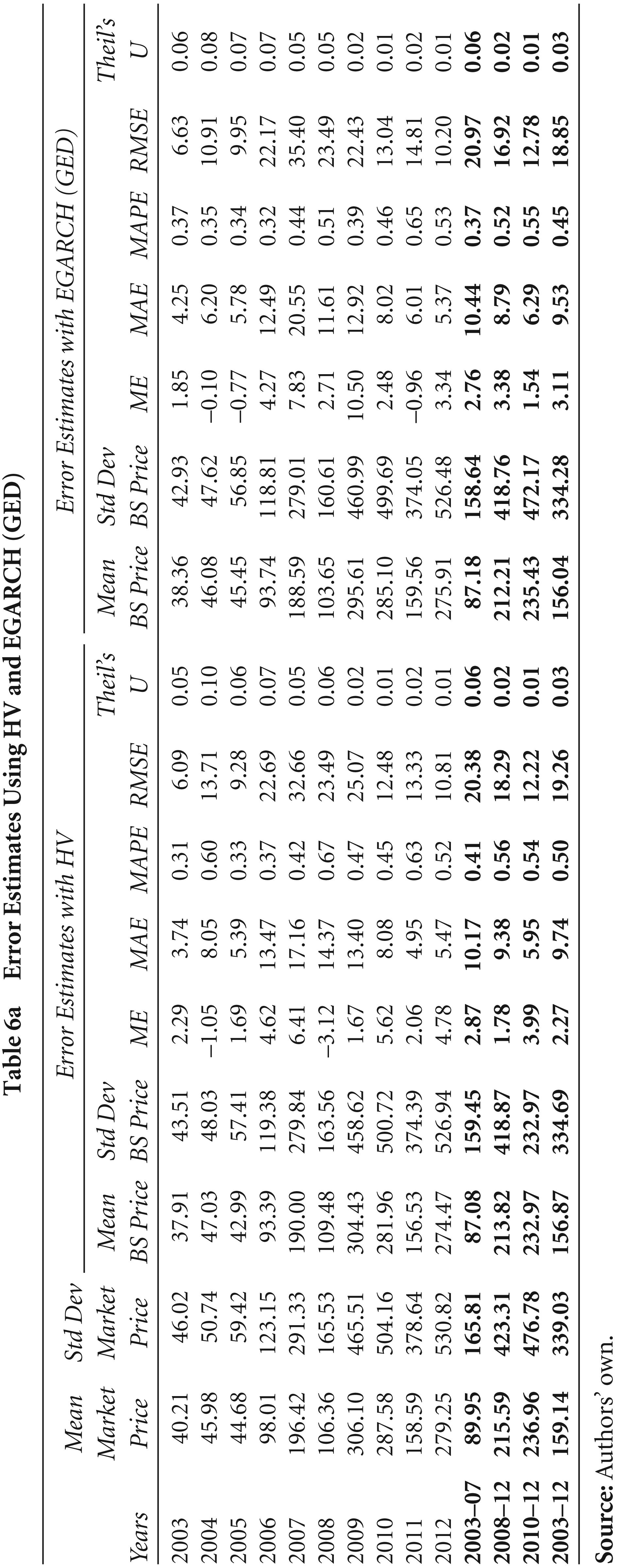
The error estimates for alternate volatility measures are presented in Tables 6a and 6b. The market exhibits considerable mispricing using all the methods of volatility. The overall ME is positive, indicating overpricing in the market for all the sub-periods, except for 2010–12 when the IV–VIX was the volatility estimate. The ME has reduced from ₹ 2.87 in the period 2003–07 to ₹ 1.78 in the period 2008–12 using HV, increased from ₹ 2.76 to ₹ 3.38 using EGARCH and decreased from ₹ 3.83 to ₹ 3.78 using IV–BS in the same time period. For both EGARCH and IV–BS estimates, the ME seems to improve in the last three years of the study, whereas the opposite is true in the case of HV. There is no discernible trend in the ME series using any of the volatility estimates for the 10-year period.
Error Estimates using IV–VIX and IV–BS
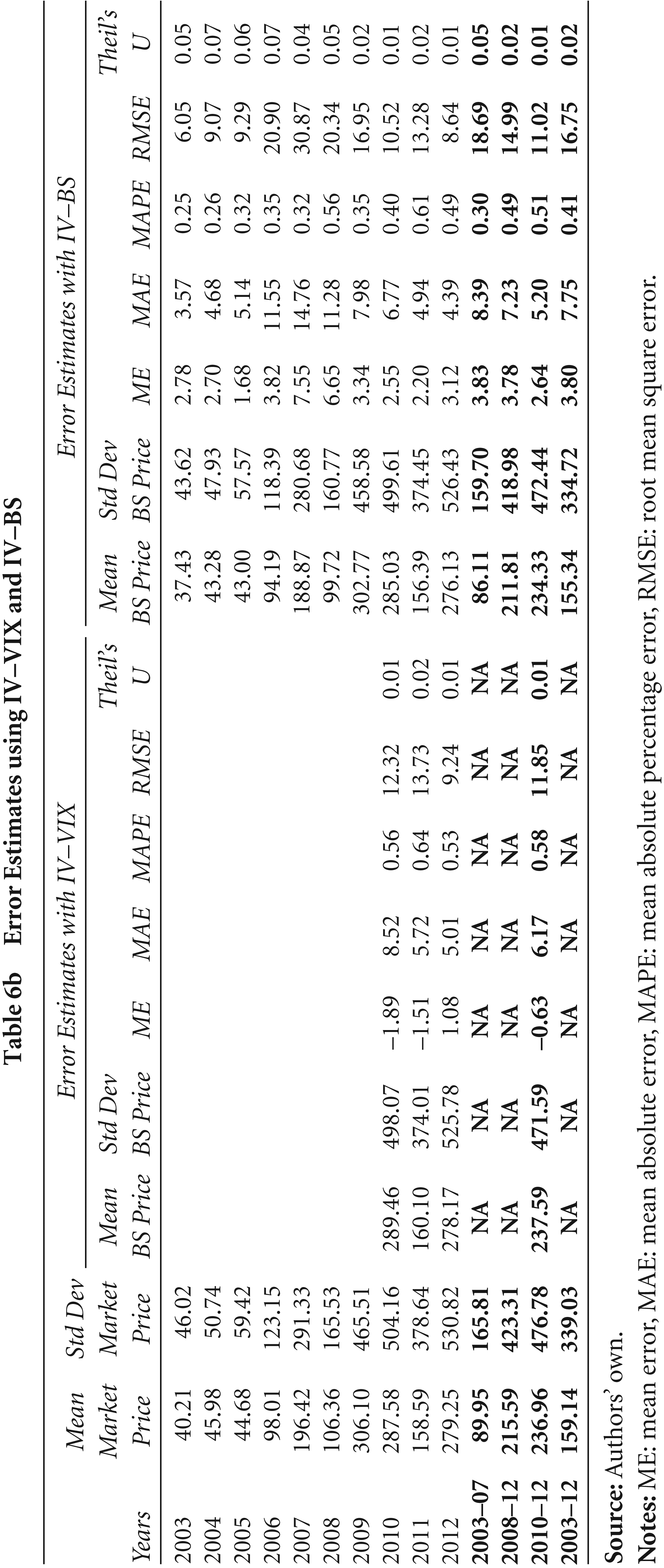
Error Estimates using IV–VIX and IV–BS
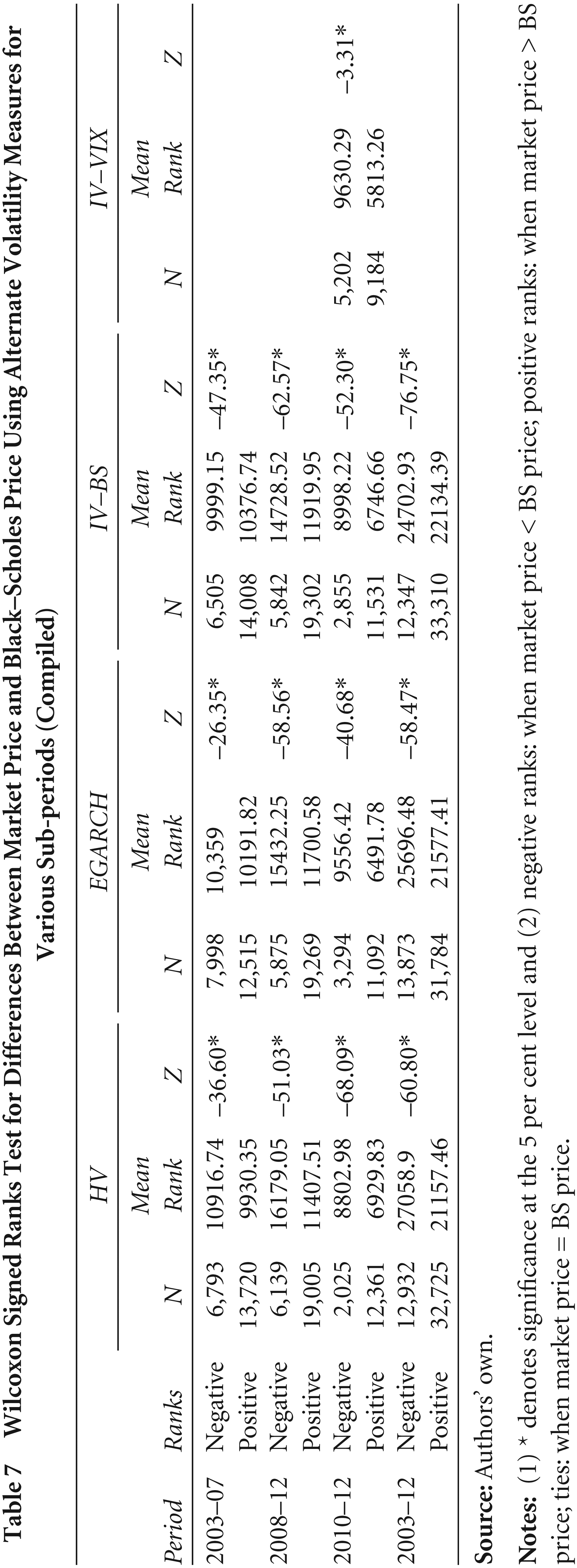
The ME series denote that there is a difference between the observed market price and the price determined by the BS model. Whether this difference is statistically significant or not needs to be validated. Since the JB test rejects the normality assumption at 5 per cent for all the methods of volatility for all sub-periods, the Wilcoxon signed rank test is applied between pairs of BS price and the observed price. It can be observed from Table 7, for all the sub-periods and with all the alternate volatility methods presently studied, the differences between the market price and theoretical price is significant at the 5 per cent level.
Wilcoxon Signed Ranks Test for Differences Between Market Price and Black–Scholes Price Using Alternate Volatility Measures for Various Sub-periods (Compiled)
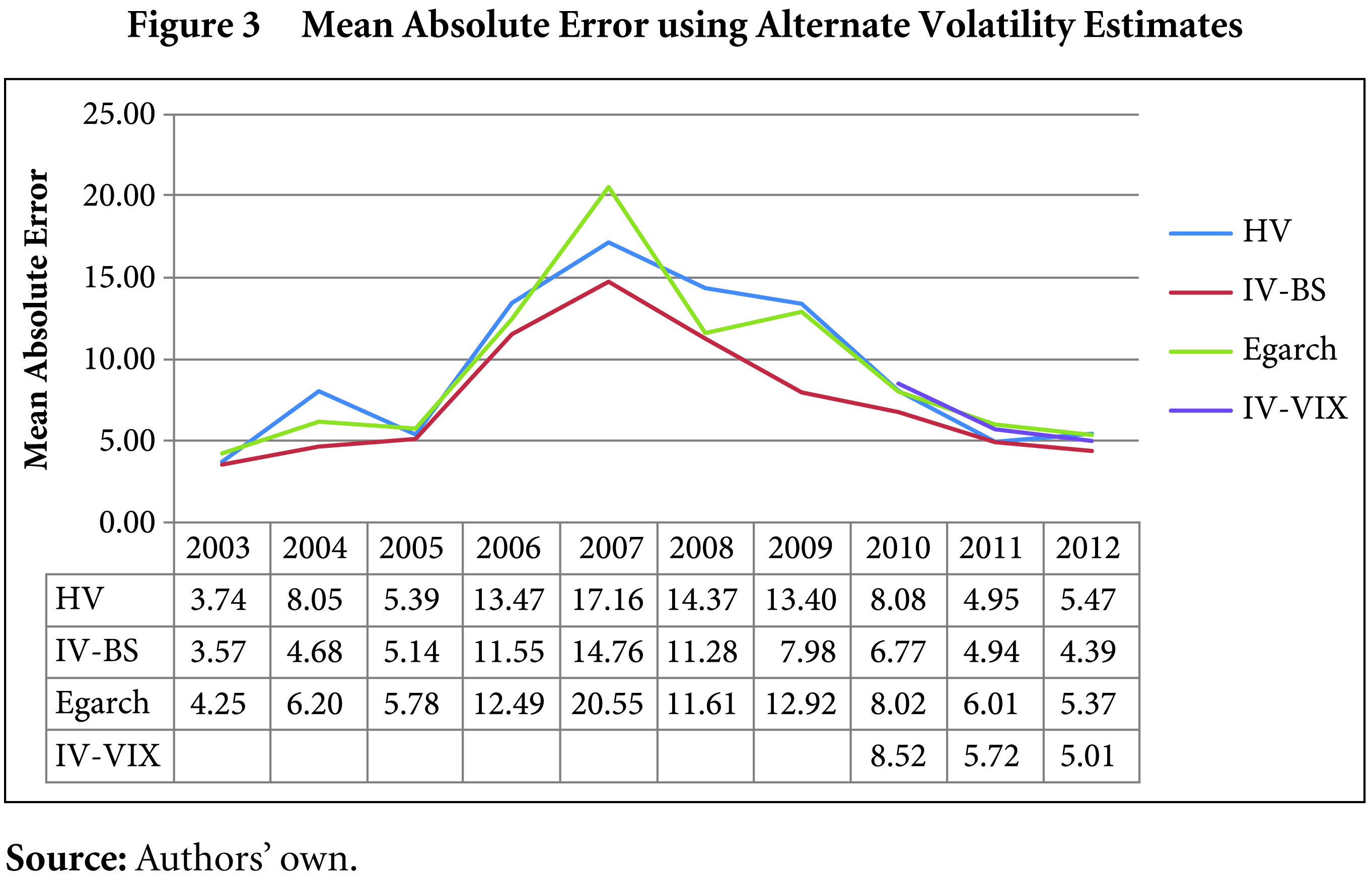
The ME tends to cancel out the negative and positive mispricing. Therefore, a study of the MAE is in order. Also, since arbitrage opportunities may arise in the case of positive violations and negative violations, the MAE is used. Overall, the MAE gives extremely encouraging results: for all the alternate methods of volatility, there is a decline in the MAE for the period 2003–07 to 2008–12. Even comparing the last five years vis-à-vis the last three years of the sample period show that there has been a decline in the magnitude of mispricing. This trend can be observed with the help of Figure 3, which illustrates that the mispricing worsened during the first five years and improved in the last five years.
A similar trend can be discerned for the RMSE. The variability in mispricing worsened in the period 2003–07 and rose almost consistently using all the methods of volatility. For 2008–12, there was a decline in the RMSE, denoting learning in the market. Both the MAE and RMSE peaked around 2007–08, which could be due to increased volatility in the markets on account of the global economic meltdown.
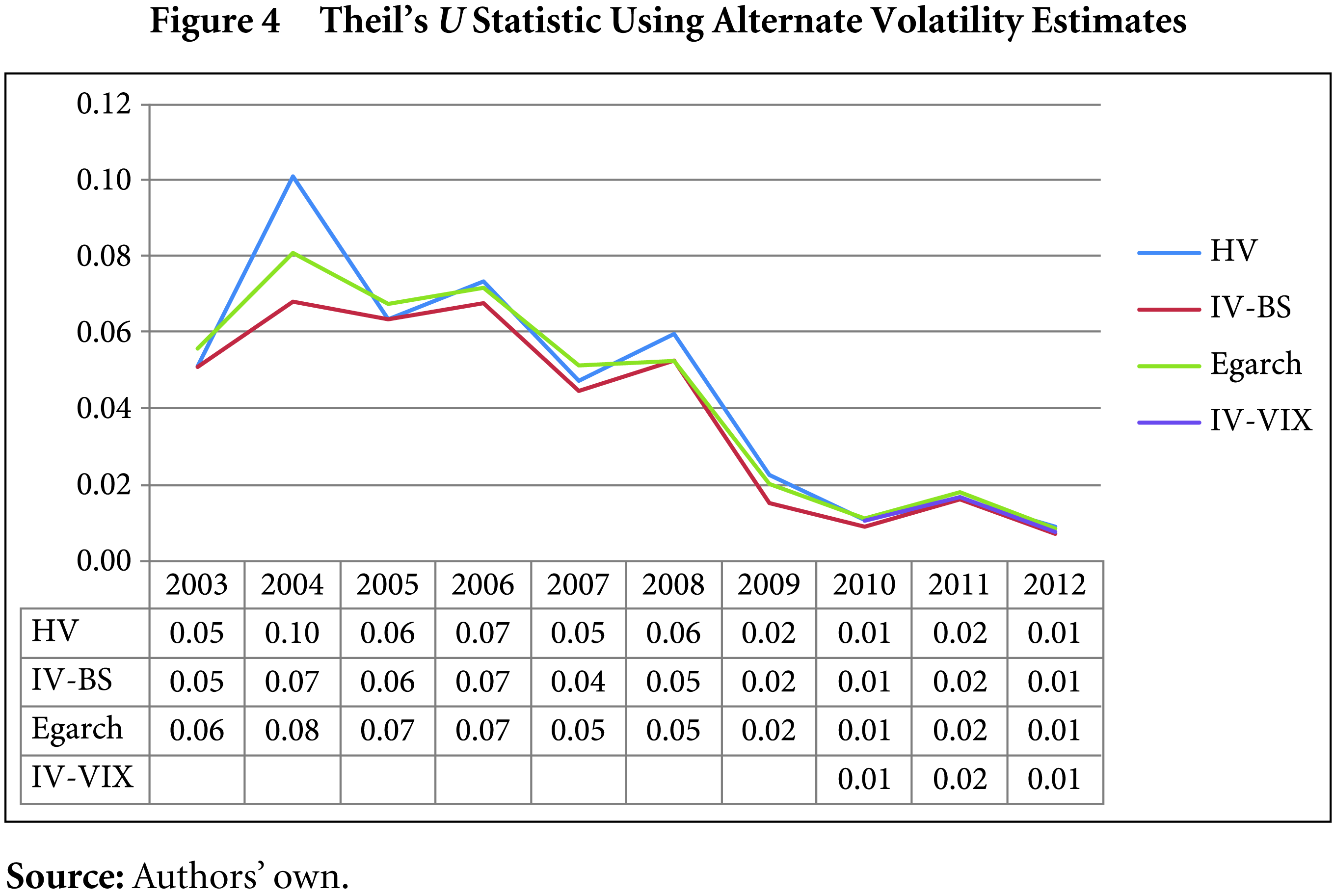
The Theil’s U statistic exhibits an overall declining trend for the 10-year study period (Figure 4). The results are almost identical using all methods of volatility up to two decimal places, indicating pricing efficiency in the CNX Nifty Index options.
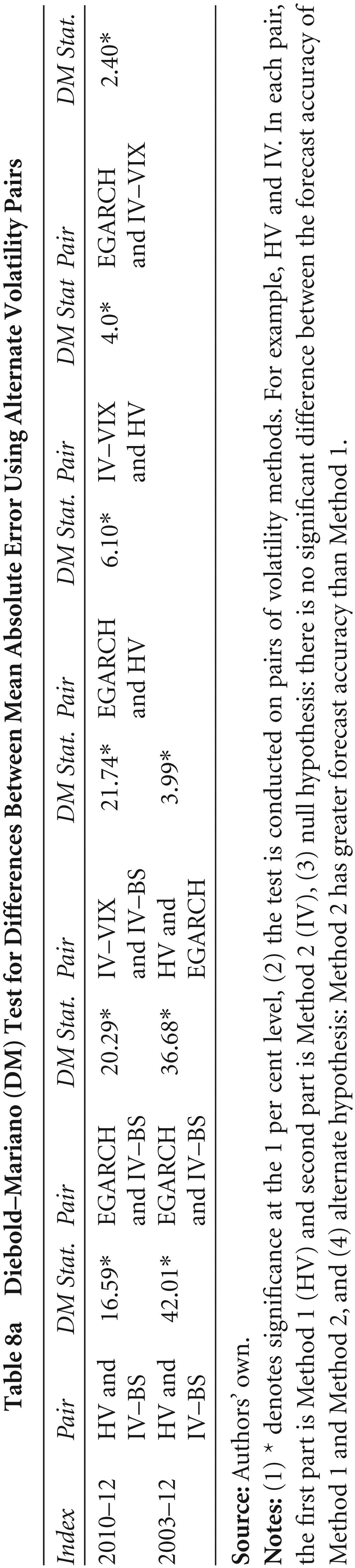
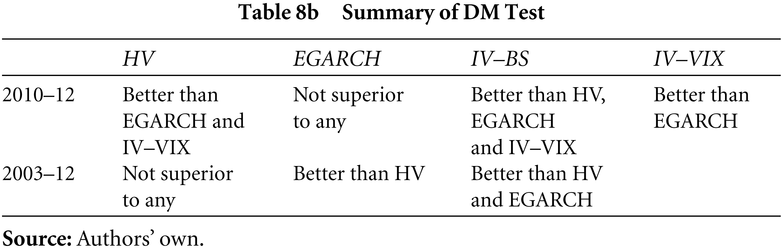
The DM test is conducted using data from the MAE series, for comparing all the pairs of volatility for the entire study period and the last sub-period (2010–12). One-tailed tests are conducted (Table 8a) and the summary is presented in Table 8b. For all the pairs, the null hypothesis is rejected at the 1 per cent significance level. Accordingly, for 2003–12, the IV–BS is superior to both the HV and EGARCH (GED), and the EGARCH (GED) is superior to the HV.
For the period 2010–12, the IV–BS is superior to all the other methods. However, the EGARCH (GED) takes a beating in comparison to both HV and VIX. This could be because conditional volatility models perform better in longer time horizons, as evidenced in the 10-year results discussed above. These results compare favourably with international studies like Christensen and Prabhala (1998), Hansen (2001), Yu et al. (2008) and Singh & Ahmad (2011a) in the Indian context, where the IV–BS consistently overperforms compared to other methods of volatility.
Diebold–Mariano (DM) Test for Differences Between Mean Absolute Error Using Alternate Volatility Pairs
Summary of DM Test
This article attempts to determine which method of volatility estimation gives a theoretical price of CNX Nifty Index options closest to the observed price. The study covers a 10-year period from 2003 to 2012. Our study indicates significant mispricing using all volatility estimates. It is encouraging to note that the magnitude of mispricing has been decreasing in the last five years of the sample period, indicating market maturity, which could be good for the overall market.
The IV as determined from the BS model proves better than all the other estimates. The EGARCH (GED) model is superior to the HV estimate in the longer run but is overcome by other estimates in short run. The supremacy of the IV in our study indicates that it is information efficient and can be used in the Indian market for forecasting volatility. The presence of the derivatives market completes the financial markets. Index options can be part of investor’s portfolio and can be used by corporates for hedging. Efficiency in pricing options contracts will lead to increased investor confidence and will be an impetus for corporates to hedge.