Impact of Age–Structure Transition on India’s Current Account Balance: An Empirical Analysis

Abstract

This article studies the impact of age structure variables on the current account balance (CAB) by using panel data for 57 countries from 1980 to 2014. The Gudmundsson and Zoega (Economic Letters 123[2]:183–186, 2014) methodology is used to calculate the age-adjusted CAB for these countries and India-specific results are analysed in comparison with Brazil, Russia, China and South Africa. Empirical results show that India’s age-adjusted CAB would have experienced surpluses had it not been for the high share of its dependent population, especially the young. Further, the age-adjustment factor for India shows a gradual decline, and a larger share of working-age population in future may help in reducing its current account deficit (CAD). These results highlight the importance of demographic variables in explaining and predicting changes in the CAB and its implication for the attainment of India’s macroeconomic objective of external stabilisation.

JEL Classification: E21, F32, J11

Keywords

Current Account Balance Age Structure Transition Age-adjusted Current Account India BRICS

1. Introduction

Demographic factors have recently received global attention in macroeconomic studies, as changes in age structure and population ageing have had a profound impact on the fiscal and other macroeconomic conditions.* Falling fertility rates and increasing life expectancy have propelled developed economies towards an ageing society, whereas these changes have created more favourable conditions for developing nations in terms of a demographic dividend.¹ Most countries in the Asian continent are experiencing a higher share of working-age population than that of children and elderly, which is expected to propel them towards higher economic growth (Asian Development Bank, 1997; Bloom & Williamson, 1998). The World Bank’s Global Monitoring Report (2015) stresses on ensuring the right set of policies in the era of intense demographic change in order to achieve sustained development and improved well-being.

This article provides an economic analysis of the relationship between age structure transition variables and the current account balance (CAB) for India, by answering the following research questions. Does the age structure transition have a role in achieving external stabilisation (gradual decline in the ratio of the current account deficit (CAD) to national income—CAD/GDP)? If yes, what is the nature and extent of this impact?

This article models and estimates age structure transition as a key determinant of the CAB. The empirical model evaluated is a panel data model of 57 countries. Using the Gudmundsson and Zoega (2014) methodology, the age-structure adjusted CAB is calculated. The results are separately analysed for the countries in the sample by classifying them into different income groups and Brazil, Russia, India, China and South Africa (BRICS). Further, using panel data estimates and India’s data, India-specific results are obtained and implications for its external stabilisation are analysed. The entire approach, results and implications add to the existing empirical analysis of India’s CAB as it is related to age structure transition.

2. Review of Related Literature

Numerous studies have focused on the impact of changes in a country’s age structure on its macroeconomic variables such as fiscal indicators (Lee & Edwards, 2002; Narayana, 2014), economic growth (Bloom & Williamson, 1998; Bloom, Canning, Fink, & Findley, 2007; Mason, 1988; Narayana, 2015a, 2015b), savings, investments and capital flows (Domeij & Floden, 2006; Feroli, 2003; Higgins, 1998; Leff, 1969; Lindh, 1999; Mason, Lee, & Jiang, 2016).

The following provides a foundation for linking demographic variables to CABs through changes in savings and investments. Under the National Income Accounting Framework, gross domestic product (GDP) from the expenditure side includes private consumption (C), gross investments (I), government consumption (G) and net exports (X – M).

G D P = C + I + G + (X - M)

(1)

which can be decomposed on the basis how it is earned and disposed in the form of consumption (C), savings (S) and taxes (T).

G D P = C + S + T

(2)

Equating (1) and (2) and subtracting C from both sides and rearranging:

S + (T - G) - I = X - M

(3)

where the (T – G) component shows public sector² savings or dis-savings, that is, (T – G) > 0 budget surplus, < 0 budget deficit and = 0 balanced budget. Thus S + (T – G) can be defined as aggregate national savings (NS).

N S + S + (T - G)

(4)

Equations (3) and (4) are used to define the CAB:

N S - I = C A B

(5)

Equation (5) indicates that national savings minus investments is equal to the CAB, which is an accumulation of claims on the rest of the world. This implies that national savings is either used for investment in the domestic economy or for stock of foreign claims. Higher savings imply a surplus in the current account. Thus, savings play a vital role in determining the current account surplus or deficit in the economy and positive net savings is an important determinant of the level of current account surplus.

The savings–investment approach to the CAB is used to link age structure transitions to current account movements. It attempts to capture the indirect impact of the age structure on the current account through the savings rate. The study by Leff (1969) established a relationship between dependency rates and savings rates in a cross-section of 74 countries stating that higher dependency rates reduced the savings rate. The study by Modigliani (1975) on the life cycle hypothesis states that savings patterns change over the life cycle of an individual, implying that a country with a large share of its population in a particular age cohort will follow similar savings rate. A larger proportion of population in working-age cohort will tend to save more as compared to young or elderly population. Fry and Mason (1982) found the existence of a level and timing effect for savings, suggesting that, savings increase with age, but the timing of the savings is dependent on the young population. Higher the young dependency ratio, lower are the savings rates as savings are postponed, in order to meet the consumption needs of the young. The NCAER study by Shukla (2010) analysed the income, consumption and savings patterns in rural and urban households in India. It indicated that household savings increased with an increase in the age of the main earning member of the household.

Taylor (1995) analysed the impact of demographic variables on savings and investments using macroeconomic panel data for Latin American countries from 1965 to 1989. The study used the Fry and Mason (1982) framework and estimated the impact of population shares of young (0–14), working age (15–64) and elderly (65 and above) on private consumption, investment and public consumption. The results suggest that the young population had the highest negative impact on private consumption, whereas those in the working age had higher savings. In the case of investments, a large share of the working-age population had strong positive impact, whereas a negative impact was observed for the elderly. With respect to public consumption, positive effects were associated with the working-age population and negative effects with the young and elderly population. The study on the basis of these findings suggested that Latin American countries could increase their current account surpluses by promoting savings during the working ages.

The study by Higgins (1998) established that higher young and elderly dependent ratios reduce savings and exacerbate CADs, based on an analysis of 100 sample countries from 1960 to 1989, by estimating a fixed effects model. The study tests the demographic effects on savings, investments and the current account. The major empirical results reveal that a higher share of the young population (0–24 years) had lower savings and higher investments, and therefore higher CADs for countries with large young dependent populations. Using the empirical framework of Higgins (1998), Lindh and Malmberg (1999) analysed the demographic effects on the savings, investment and current account for 20 OECD countries by using panel data from 1960 to 1994. The results suggested that the young and elderly reduced savings, which was similar to the results obtained from the world samples by Higgins (1998), but the effects on investment were different. The study used disaggregated investment to capture the demographic effects and found that young cohorts had a positive correlation with housing investment, whereas mature cohorts were positively correlated with business investments.

Herbertsson and Zoega (1999) incorporated the working-age population to determine private savings and government savings and established that the existence of current account imbalances partly reflects demographic differences across countries. They used Modigliani’s life cycle hypothesis to model the behaviour of the current account by using data for 84 countries for the period 1960–1990. Combining the life cycle hypothesis with the national income account identity, the study tests the hypothesis that a nation with a higher share of working-age population would have a current account surplus, while a country with a larger share of young and retired people would run CADs. They extended their analysis to bring out the direct effect of the age structure on the current account through private savings, differentiating it from the government budget surplus. The empirical results state that the working- age population and budget surplus account for 31 per cent of the variations in the current account; one-fourth of the effects of the demographic variable work through the public budget, whereas three-fourths work through private savings. Kim and Lee (2007) using panel data comprising ten East Asian countries and Kim and Lee (2008) using data for a group of seven advanced nations (G7) find similar results, indicating that increasing dependency rates lead to a decline in savings rates and thereby worsens CABs. Kim and Lee (2008) use panel VAR to capture the demographic affects and conclude that rising dependency rates have a detrimental impact on public savings.

Gudmundsson and Zoega’s (2014) panel data study subtracted age effects from the current account to obtain the age-adjusted current account for 57 nations for the period 2005–2009. They found that demographics and age structure have a significant impact on CABs. The age-adjusted CAB showed that countries with high dependent populations, such as Japan and Germany, had diminished current account surpluses, whereas surpluses in China, Malaysia and Singapore were high due to their larger proportion of working-age population. Using the fixed effects regression model with the current account as a percentage of GDP as the dependent variable and the share of population under 0–24 years (young) and 65 years and above (elderly) as independent variables, the study offered evidence that both these demographic variables had a negative impact on current account surpluses.

Studies by Debelle and Faruqee (1996), Chinn and Prasad (2003) and Gruber and Kamin (2007) included demographic variables (expressed as dependency ratios) along with other macroeconomic determinants of the CAB such as exchange rates, fiscal balance, trade openness, GDP growth and business cycles, to analyse the impact of these variables on the CAB. Their studies also provide evidence that dependent populations, that is, the young and elderly, have a negative impact on the CAB.

External stabilisation, that is, reducing the CAD-to-GDP ratio, has been a key policy agenda for the Indian economy, especially after the 1990s balance of payments (BOP) crisis. In general, India’s external sector policies use traditional, conventional approaches to explain and predict CADs, including exchange rates and inflation (Rangarajan & Mishra, 2013), budget deficits (Bose & Jha, 2011) and openness to trade and trade barriers (Panagariya, 2004). In the approaches to analysing the CAB for India, demographic variables do not find an explicit role, and this article attempts to address this lacuna.

3. Trends in India’s Current Account Balance and Its Age Structure Transition

3.1 Trends in the Current Account Balance

India follows the IMF classification to record economic transactions in current account.³

The total on the BOP account is the sum of the current and capital account balances. A positive overall balance for India is due to the high inflow of foreign funds in its capital account which offsets the negative balance in its current account. India’s BOP deficit of US$962.6 million for 1980–1981 to 1984–1985 was high due to deficits in its current account and insufficient capital inflows (Table 1). In the subsequent periods, there is higher inflow of capital over and above the CAD, especially from the period 2000–2001 to 2004–2005. The period 2005–2006 to 2009–2010 saw the highest surplus in the BOP (US$27,436.6 million) even though the current account for that period escalated to an average deficit of US$20,260 million due to a surge in capital inflows. The period 2010–2011 to 2014–2015 experienced high CADs on account of increased gold and oil imports. India’s overall BOP position has remained positive since 1990–1991, due to the inflow of foreign capital greater than the amount required to pay for imports in excess of exports, which has led to high foreign exchange reserves.

Table 1
India’s Balance of Payments by Current and Capital Account 1980–1981 to 2014–2015

Time Period Current Account (US$ million) Capital Account
(US$ million) Balance of Payments
(US$ million)

1980–1981 to 1984–1985 −3004.6 2042.2 −962.6

1985–1986 to 1989–1990 −5823.4 5821.2 −1.8

1990–1991 to 1994–1995 −3782.4 6550.2 2,767.8

1995–1996 to 1999–2000 −4953.2 9094.4 4,141.2

2000–2001 to 2004–2005 3738.4 14699.6 18,438

2005–2006 to 2009–2010 −20,260 47696.8 27,436.6

2010–2011 to 2014–2015 −54,941 71133.2 16,191.8

Time Period	Current Account (US$ million)	Capital Account (US$ million)	Balance of Payments (US$ million)
1980–1981 to 1984–1985	−3004.6	2042.2	−962.6
1985–1986 to 1989–1990	−5823.4	5821.2	−1.8
1990–1991 to 1994–1995	−3782.4	6550.2	2,767.8
1995–1996 to 1999–2000	−4953.2	9094.4	4,141.2
2000–2001 to 2004–2005	3738.4	14699.6	18,438
2005–2006 to 2009–2010	−20,260	47696.8	27,436.6
2010–2011 to 2014–2015	−54,941	71133.2	16,191.8

Source: Reserve Bank of India (2015).

Note: Data pertains to the fiscal year (1 April–31 March).

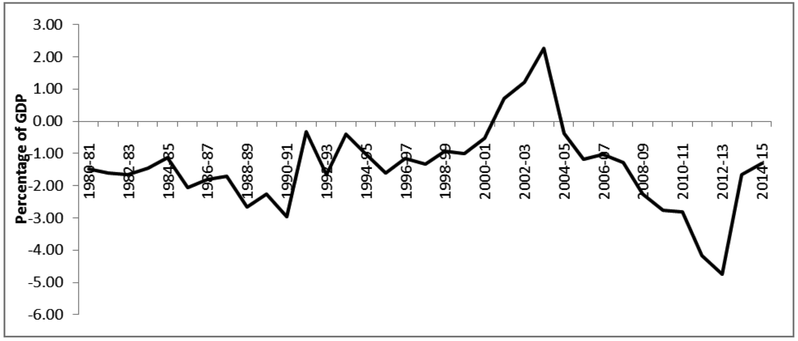
The current account as a percentage of the GDP was −1.5 during 1980–1981 and deteriorated to –3 per cent in 1990–1991 during the BOP crisis (see Figure 1). With the introduction of economic liberalisation in 1991–1992, there was a slight improvement in the ratio, which averaged around −1.14 per cent in 1992–2000. Apart from the 4 years in the early 2000s (2000–2003), India had not experienced a current account surplus in the last 35 years. The surplus peaked at 2.2 per cent in 2003–2004 due to strong exports and a boom in IT trade and recorded a low of −4.7 per cent in 2012–2013 due to a decrease in global economic activity, an increase in oil prices, high gold imports and a depreciated Indian rupee. The CAD for 2014–2015 was −1.4 per cent of GDP; India’s average CAB-GDP ratio from 1980 to 2015 was −1.47 per cent.

Figure 1

Source: Reserve Bank of India (2015).

3.2 Age Structure Transition

India’s population is experiencing a change in its age structure with an increase in the proportion of people in the working-age group and a smaller proportion of population in the young and elderly categories. The main reason for the decline in the young population is the fall in fertility rates. The total fertility rate (TFR) declined from 5.87 children per woman at the beginning of the 1960s to 2.4 in 2014 (World Bank, 2016) and is predicted to decline further in the coming decades.

Figure 2

Source: World Bank (2014).

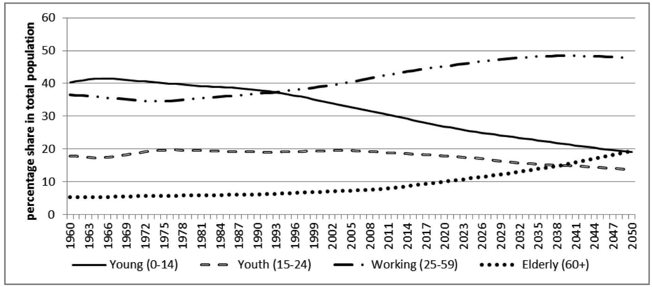
The share of the young population in total population has reduced from 40.3 per cent in 1960 to 29.2 per cent in 2014 and is projected to further decline to 19.1 per cent in 2050 (Figure 2). The youth population was stagnant at approximately 20 per cent of the total population till 2010, after which it declined and is projected to shrink to 13.7 per cent by 2050. The share of the elderly in the total population is expected to expand: people above the age of 60 were only 5.2 per cent of the total population in 1960, but in 2014 they were 8.6 per cent, and for 2050 they are projected to be close to 20 per cent. The share of the working population increased from 36.5 per cent in 1960 to 43.5 per cent in 2014, and by 2050 it will be 47.8 per cent. It is interesting to note that during 1991–1992 there was a crossover between the young and working-age population shares: a scissor shape is observed between the two curves, highlighting that since 1991 there has been a marked decline in the share of the young population and a rise in the share of the working-age population.

4. Methodology

The Gudmundsson and Zoega (2014) model is extended by the study period and by drawing country-specific implications for India. The empirical model and estimation technique is given below.

4.1 Model

C A B_{i t} = α + β_{1} P y_{i t} + β_{2} P o_{i t} + δ_{1} g r o w t h_{i t} + δ_{2} P y_{i t} * g r o w t h_{i t} + U_{i t}

(6)

CAB is taken as a percentage of GDP, P_y and P_o are demographic variables, percentage of young population (24 years and below) and elderly (65 years and above), respectively; the middle age (25–65 years) is not included to avoid perfect multicollinearity. Following Fry and Mason (1982), the ‘growth’ variable, which is the growth rate of income per capita, and P_y*growth, the interactive term between growth and young variables, are used to capture the level and timing effects on savings, respectively, because the young population enjoys higher income and consumption with an increase in economic growth. The variable rate of growth effect model studies the nexus between youth dependency and the national savings rate. Positive labour productivity growth implies that the younger generation has higher permanent income and consumption compared to their elders. The savings rate depends on the interaction between the youth dependency ratio and growth rate of national income, the logic being that a declining youth population will shift consumption from the child-rearing stages to the non-child-rearing stages (Higgins, 1998). For example, in a country with a large young population, the working-age cohort will save less as they would have to provide for the young; thereby the country would have a lower current account surplus, compared to a country which has a smaller youth-dependent population, as its working-age population would have a lower burden of providing for the young and can save more.

4.2 Prediction

The predicted signs on the coefficients are as follows:

αβ1β2δ1δ2

The expected signs of the standardised coefficient for the constant term (α) must be positive as it captures the impact of the working-age population, which contributes positively towards the current account; the coefficients of the demographic variables (β1) and (β2) must be negative as both the young and the elderly adversely impact the CAB; the coefficient of growth variable (δ1) and interaction term (δ2) must have negative signs too, as higher levels of income lead to higher consumption in the presence of a high dependent population.

4.3 Calculation of the Age-adjusted CAB

Using panel data, pooled OLS and a fixed effects model are estimated by including or excluding the growth and interaction terms and the F-test is conducted to choose between the fixed effects model (FEM) and the pooled regression model (PRM) on empirical grounds. The coefficients estimated through the fixed effect model without the growth and interactive term is used to calculate the age-adjusted CAB for 57 countries. Following Gudmundsson and Zoega (2014) age-adjusted CAB is calculated by taking the average of the two population variables (young and elderly) and the CAB from 2009–2014 as $\bar{P} $ _y, $\bar{P} $ _o and $\overset{─}{C A B}, $ respectively, and the estimated coefficients $\hat{β} $ ₁ and $\hat{β} $ ₂ are multiplied with $\bar{P} $ _y and $\bar{P} $ _o which are the averages of P_y and P_o for the years 2009–2014, to obtain Z*.

Z^{*} = {\bar{P}}_{y} * {\hat{β}}_{1} + {\bar{P}}_{o} * {\hat{β}}_{2} ​ ​

(7)

A g e ​ - ​ A d j u s t e d C A B = (\overset{─}{C A B} - Z^{*}) - α ​

(8)

A d j u s t m e n t f a c t o r = A g e ​ - ​ A d j u s t e d C A B - \overset{─}{C A B} ​

(9)

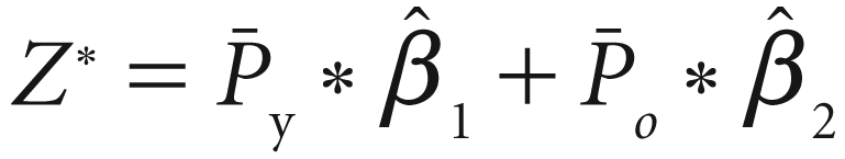
The age-adjusted CAB is calculated from $\overset{─}{C A B} $ by subtracting Z* and the constant term (α). The Adjustment factor is the difference between age-adjusted CAB and $\overset{─}{C A B} $ which shows the nature and impact of the age structure on the CAB.

4.4 Country-specific Implications

The implications for India are calculated from the cross-country estimation in Equation (6) without the growth and interactive terms. The India-specific age-adjusted CAB was obtained as:

Z_{t}^{I} = P_{y, t}^{I} . {\hat{β}}_{1} + P_{o, t}^{I} . {\hat{β}}_{2} (t = 1980, 1981, 1982 \dots \dots .2014) ​

(10)

A g e ​ - ​ A d j u s t e d C A B_{t}^{I} = (C A B_{t}^{I} - Z_{t}^{I}) - α ​

(11)

A d j u s t m e n t F a c t o r = A g e A d j u s t e d C A B_{t}^{I} - C A B_{t}^{I} ​

(12)

In Equations (7)–(9), the age-adjusted CAB is calculated for all 57 nations using the average of CAB, P_y and P_o for the years 2009–2014, whereas for Equations (10)–(12), the age-adjusted CAB is calculated for the entire period from 1980–2014 for a country-specific analysis. This captures the year-wise changes in the impact of age structure transition on the CAB for India; the adjustment factor is calculated for each year to highlight its movement over the period.

4.5 Variables and Data Description

Table 2 lists the variables and their sources that are employed in the estimation of the panel regression models described in the previous sections.

Table 2
Variable Description and Data Sources

Variable Measurement Data Source

Current account balance CAB Percentage of GDP at current prices RBI (2015)
IMF (2015)

Young population P _y Population aged 0–24 years as a percentage of total population World Bank (2014)

Elderly population P _o Population aged 65 years and above as a percentage of total population

Per capita growth rate growth Growth rate of per capita GDP in current prices IMF (2015)

Interaction term P_y**growth*

Variable		Measurement	Data Source
Current account balance	CAB	Percentage of GDP at current prices	RBI (2015) IMF (2015)
Young population	P _y	Population aged 0–24 years as a percentage of total population	World Bank (2014)
Elderly population	P _o	Population aged 65 years and above as a percentage of total population
Per capita growth rate	growth	Growth rate of per capita GDP in current prices	IMF (2015)
Interaction term	P_y*growth

Source: The author.

5. Empirical Results

This section discusses the estimation results separately for the cross-country analysis and the India-specific analysis.

5.1 Cross-country Evidence

The estimation results of the panel regression (57 countries over 34 years) in Equation (6) are presented in Table 3.

Table 3
Age Structure Transition Effects on the Current Account, 1980–2014

Variables Models

Dependent variable: CAB PRM FEM (1) FEM (2)

Young (0–24) −0.497*
(−15.46) −0.425*
(−8.48) −0.441*
(−8.50)

Elderly (65+) −0.955*
(−13.83) −0.668*
(−5.70) −0.69*
(−5.80)

Growth per capita −35.606
(−2.88) −26.141
(−1.77)

Growth * young 0.66
(2.28) 0.529
(1.54)

Constant 29.96*
(14.89) 23.731*
(7.5) 24.696*
(7.56)

R ² 0.117 0.462 0.464

F-statistic 60* 35.71* 34.37*

Number of observations 1,804 1,804 1,804

F-test for fixed effects F(56, 1745) = 20.28* F(56, 1743) = 20.15*

Variables	Models
Young (0–24)	−0.497* (−15.46)	−0.425* (−8.48)	−0.441* (−8.50)
Elderly (65+)	−0.955* (−13.83)	−0.668* (−5.70)	−0.69* (−5.80)
Growth per capita	−35.606 (−2.88)		−26.141 (−1.77)
Growth * young	0.66 (2.28)		0.529 (1.54)
Constant	29.96* (14.89)	23.731* (7.5)	24.696* (7.56)
R ²	0.117	0.462	0.464
F-statistic	60*	35.71*	34.37*
Number of observations	1,804	1,804	1,804
F-test for fixed effects		F(56, 1745) = 20.28*	F(56, 1743) = 20.15*

Source: Author’s estimation based on Equation (6).

Notes: ^*Denotes significance at the 1 per cent level; values in parenthesis for variables are the t-statistics.

The F-test for poolability⁴ shows that countries are not poolable and that the fixed effects model is empirically appropriate and statistically significant.

Table 3 shows that the standardised coefficients have the expected signs. In all three estimated models {PRM, FEM (1) and FEM (2)}, the young and the elderly exhibit a negative impact on the CAB.⁵ Using the life cycle hypothesis and savings–investment approach, it can be stated that the young and the elderly reduce the current account surplus because they consume/dis-save more than they earn. The choice between the FEM (1) and FEM (2) models is based on qualitative differences. First, the growth and interaction variable are not statistically significant in FEM (2). Second, standardised coefficients of the population variables (Young and Elderly) in FEM (1) are not significantly different after the incorporation of the growth and interaction variable in FEM (2). Thirdly, incorporation of the growth and interaction term did not improve the R² for FEM (2). The standardised coefficients of the FEM (1) are used to calculate the age-adjusted CAB.

Table 4 gives the results of the nature and extent of the age-adjusted CAB for 57 countries for the period 2009–2014. The countries are classified into surplus and deficit countries based on their actual CAB. The World Bank classification (July 2013)⁶ of countries based on income is adopted, which groups countries into high income, upper middle income, lower middle income and low income countries based on their per capita incomes.

Table 4

Actual and Age-adjusted Current Account Balances, Surplus and Deficit Countries, 2009–2014

High Income	Actual CAB	Adjusted CAB	Adjustment	Upper- Middle Income	Actual CAB	Adjusted CAB	Adjustment	Lower-Middle Income	Actual CAB	Adjusted CAB	Adjustment
Surplus Countries
Singapore	19.44	15.1	−4.34	Malaysia	8.16	7.49	−0.67	Philippines	3.76	5.29	1.53
Saudi Arabia	15.37	13.45	−1.92	China	2.8	−0.87	−3.67
Norway	10.96	10.95	−0.01	Thailand	2.52	−1.09	−3.61
Switzerland	9.88	9.06	−0.82	Hungary	1.67	0.67	−1
Netherlands	9.05	8.62	−0.43
Sweden	6.39	7.87	1.48
Germany	6.34	6.83	0.49
Luxembourg	5.98	4.1	−1.88
Denmark	5.65	6.36	0.71
Honk Kong SAR	4.57	0.13	−4.44
Korea Rep	4.1	0.58	−3.52
Russia	3.67	1.03	−2.64
Israel	3.04	4.47	1.43
Slovenia	2.45	0.74	−1.71
Japan	1.91	3.99	2.08
Austria	1.72	1.39	−0.33
Ireland	0.58	−1.13	−1.71
Estonia	0.37	0.45	0.08
Belgium	0.05	0.23	0.18
Deficit Countries
Latvia	−0.2	0.08	0.28	Argentina	−0.21	0.97	1.18	Indonesia	−1.01	−1.98	−0.97
Lithuania	−0.26	0.19	0.45	Mexico	−1.38	−0.74	0.64	Pakistan	−2	1.28	3.28
Finland	−0.71	−0.16	0.55	Bulgaria	−1.47	−2.03	−0.56	India	−2.95	−2.31	0.64
France	−0.94	0.08	1.02	Peru	−2.61	−1.83	0.78	Ukraine	−5.33	−7.08	−1.75
Croatia	−0.95	−1.27	−0.32	Columbia	−3.23	−4.23	−1	Morocco	−6.75	−6.58	0.17
Chile	−0.98	−2.09	−1.11	Romania	−3.25	−4.41	−1.16
Italy	−1.01	−0.61	0.4	Brazil	−3.25	−4.6	−1.35
Spain	−1.57	−3.08	−1.51	South Africa	−3.76	−2.63	1.13
Czech Rep	−1.61	−3.41	−1.8	Turkey	−6.28	−6.66	−0.38
Slovak Rep	−1.78	−4.76	−2.98
United States	−2.65	−3.13	−0.48
Iceland	−2.77	−3.06	−0.29
Canada	−2.91	−4.18	−1.27
New Zealand	−2.97	−2.88	0.09
Poland	−3.41	−5.74	−2.33
United Kingdom	−3.53	−3.03	0.5
Australia	−3.66	−4.15	−0.49
Portugal	−4.44	−4.41	0.03
Greece	−5.31	−5.12	0.19

Source: Author’s calculations based on equations (7)–(9) and estimated results from Table 3, FEM (1); World Bank (2013).

Notes: Classification of countries into income groups are according to 2012 gross national income (GNI) per capita, calculated using the World Bank Atlas method. The groups are: low income, US$1,035 or less; lower-middle income, US$1,036–4,085; upper-middle income, US$4,086–12,615; and high-income, US$12,616 or more.

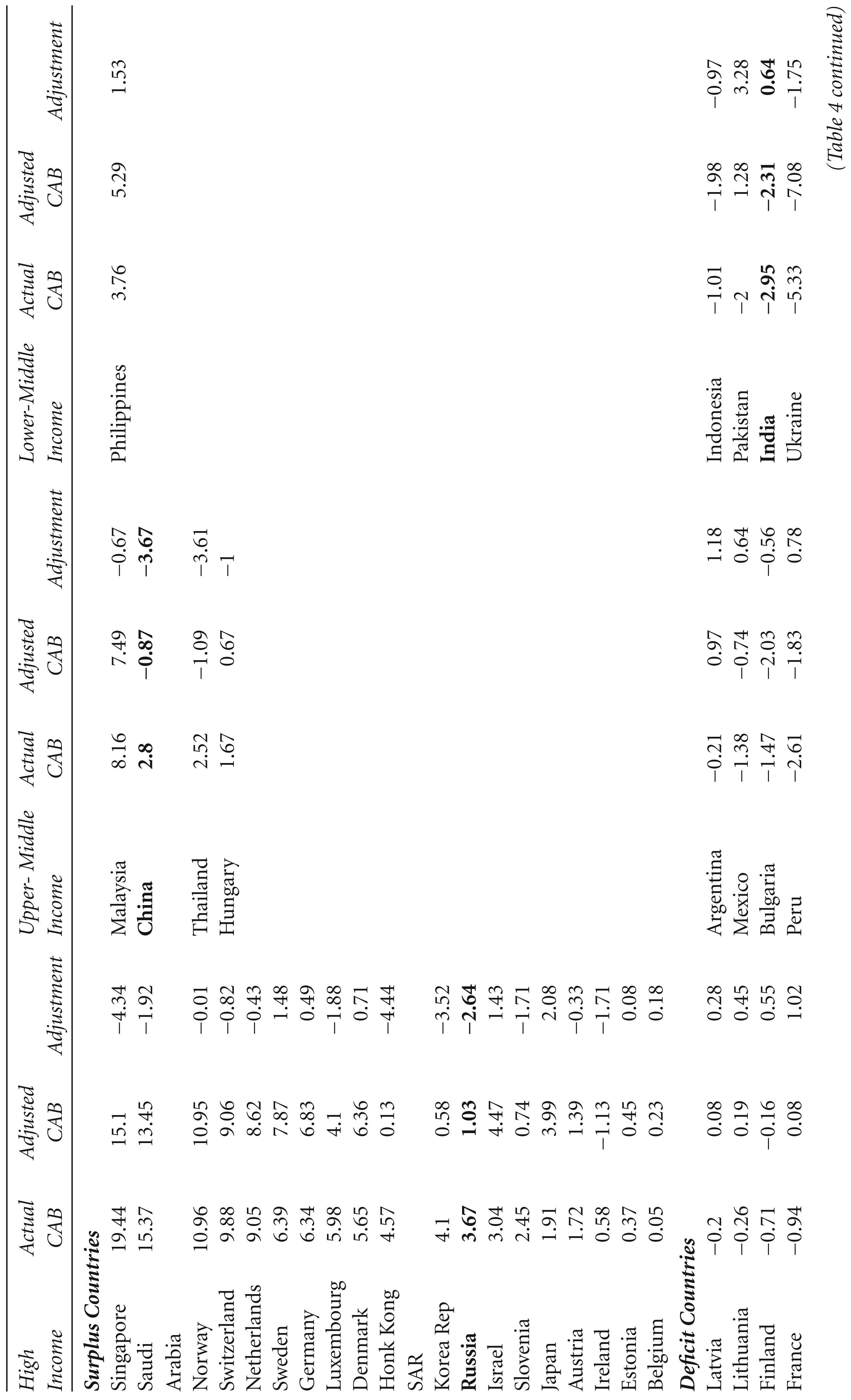
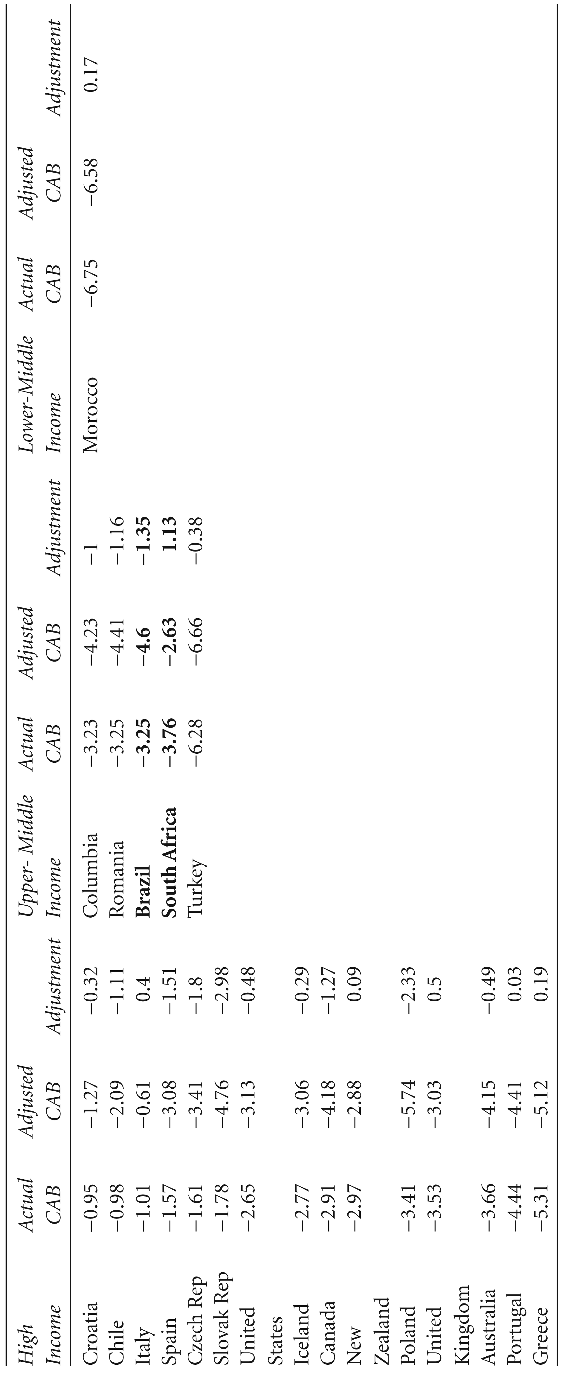
A negative adjustment implies that there is a high share of the working-age population in the economy, while a positive adjustment indicates a large share of dependent (young and/or old) population. Among the High Income and Surplus Countries, Singapore, Hong Kong SAR, Republic of Korea and Russia have a high negative adjustment due to a high share of working-age population in these countries. Once the adjustment is netted out of the actual CAB as a per cent of GDP, the current account surpluses reduce drastically—for Hong Kong SAR by −4.44 per cent, Singapore by −4.34 per cent, Korea Republic by −3.52 per cent and for Russia by −2.64 per cent. Japan, Sweden, Israel, Denmark and Germany have a positive adjustment, as they have a high share of older population; Japan and Sweden’s adjusted CAB as a per cent of their GDP increased by 2.08 per cent and 1.48 per cent, respectively.

Among the high income and deficit countries, France, Finland, United Kingdom, Lithuania and Italy have a positive adjustment on account of their older populations, and countries such as the Slovak Republic, Poland, the Czech Republic, Canada, Chile and Spain have a negative adjustment depicting high share of working-age populations.

Among the Upper-Middle Income Countries, China has the highest negative adjustment of −3.67 per cent followed by Thailand (−3.61 per cent). Once the adjustment is taken into account, China’s current account surplus of 2.8 per cent of GDP shifted into a deficit of −0.87 per cent and Thailand’s surplus shifted from 2.52 per cent to a deficit of −1.09 per cent.

Pakistan, Philippines and India have positive adjustment factors, as they have a higher share of young people in their populations. These lower-middle income countries experienced an increase in their CABs when the age structure transition was netted out. Pakistan’s CAD of 2 per cent of GDP shifted to a surplus of 1.28 per cent after accounting for its age structure.

For India, the adjustment is positive but not of a remarkable magnitude; the positive adjustment indicates that its large dependent population (especially the young) is responsible for reducing its current account surplus by 0.64 per cent of its GDP. These results differ significantly from those obtained by Gudmundsson and Zoega (2014). In their article, India had a negative adjustment factor of −0.32, while in our analysis India has a positive adjustment factor. The positive adjustment factor is more close to theory as India has a large dependent population which must necessarily increase its deficits. Countries such as Canada, Peru and Argentina have moved into the deficit country group due to their CADs in the past 5 years, and Estonia and Ireland have become surplus nations. Austria, Norway, Bulgaria and New Zealand have had reverse adjustment factors when compared with the results of Gudmundsson and Zoega (2014). One of the reasons for the reversal of the adjustment factor could be the extension of the time period and differences in the dataset used.

Of the BRICS nations, China, South Africa and Brazil are upper-middle income Countries, Russia is a high income country and India a lower-middle income country. Not only are the incomes different among these countries, but so are their stages of age structure transition. China and Russia have a high share of working-age population which is depicted in their adjustment factor, followed by Brazil, South Africa and India. In order to understand how the age structure transition impacts the CAB over the decades, a country-specific analysis is presented in the following section.

5.2 India-specific Analysis

The impact of age structure on the CAB was calculated and presented in Table 4, but it only provides the average impact of the age structure transition on the CAB for 2009–2014. In order to bring out the impact of the age structure variables for India from 1981 to 2014 (year-wise), the actual and age-adjusted CAB are calculated using Equations (10)–(12) along with the coefficients obtained from FEM (1) in Table 3. The results are presented in Figure 3.

Figure 3 shows that if the age effect is netted out from the current account then India would have a current account surplus rather than a deficit for most of the study period. The actual CAB includes the effects of all the macroeconomic variables as well as the age effect. When the age effect is subtracted for India, a drastic shift in the CAB is observed. Thus, a country’s age structure explains to a large extent the deficits in its CABs. For the entire study period (1981–2014), the age-adjustment factor for India has been positive, implying that its high share of dependent young population has a negative impact on its CAB.

Figure 3

Source: Author’s calculations based on equations (10), (11) and (12) and estimated results from Table 3, FEM (1).

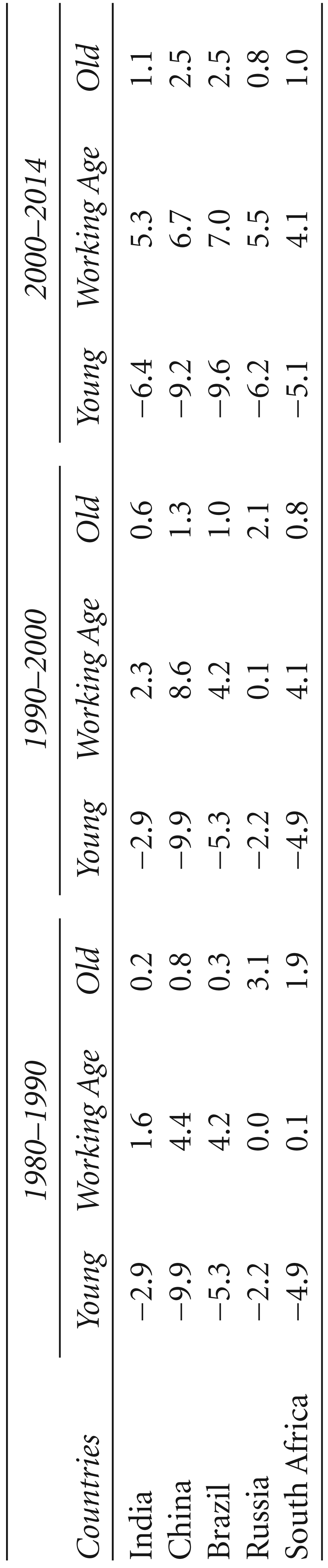
At the beginning of the 1980s, the age effect was 4 per cent, and netting out the age effect from its actual CAB yields a surplus of 2 per cent of its GDP. Due to its age structure transition, the gradual decline in the share of its young population and simultaneous increase in the share of its working-age population, the age effect fell to 3 per cent between 1991 and 1995. It further declined to 2 per cent from 1998 to 2003, and from 2005 onwards, it has tapered further to 1 per cent in 2012. The decline in the young population by 6.4 per cent from 2000 to 2014 and increase in the working-age population by 5.3 per cent during this period (Table A2) has led to a convergence between the actual and the age-adjusted CAB. For the years 2012–2014 the actual and the age-adjusted CABs have almost overlapped, depicting a negligible age effect which suggests that the negative impact on India’s CAB from its dependent population is being nullified by the positive contributions of its working-age population.

Studying the impact of the age-structure transition on India in isolation may not help in predicting the future course of its age-adjusted CAB. A comparison with other economies can shed a better light in this regard. The BRICS nations are selected as they are homogenous on the basis of economic activity and international presence and heterogeneous in age structure and income levels. Placing India alongside other emerging economies would help understand the impact of the age effect on CABs in the future.

5.3 Comparisons with other BRICS Economies

As observed in Table 4, China, Russia and Brazil have negative age-adjustment depicting a positive contribution of the working-age population, whereas India and South Africa have a positive adjustment indicating an adverse impact on their CABs due to the high share of the dependent population. Replicating the technique used to extract India’s age-adjusted CAB, that is, using Equations (10)–(12) and the coefficients obtained from FEM (1) in Table 3, the age-adjusted CABs for the rest of the BRICS nations are presented in Figure 4.

Figures 3 and 4 bring out the fact that in all the BRICS nations, except for Russia, actual CABs were below the adjusted CABs during the 1980s and the 1990s, indicating a high share of dependent populations. Brazil, China and Russia have passed the convergence phase,⁷ where the actual CAB is equal to the age-adjusted CAB. For Brazil it was during the early 2000s and for China in the mid-1990s. Brazil and China have experienced a crossover of their age-adjusted and actual CABs, which indicates that the positive contributions by the working-age population are greater than the adverse impact of the dependent population on the current account.

Prior to the convergence phase, both China and Brazil had higher age-adjusted CAB compared to their actual CAB, which shows that if the age effect was netted out, both economies would have experienced higher balances in their current account. The high dependent populations in these two countries was reducing their CABs by approximately 2 per cent of GDP for China and 3 per cent for Brazil. The fall in the dependent young population and rise in the working population brought about a convergence between the adjusted and actual CABs; China’s working population increased by 8.6 per cent and young population fell by 9.9 per cent during 1990–2000, while Brazil’s working population increased by 7 per cent during 2000–2014, and its young population shrunk by 9.6 per cent during the same period. Hence, China achieved the convergence earlier than Brazil. Today, both countries are experiencing high contributions towards their CAB from their large shares of working population—China nearly 4 per cent and Brazil by 1 per cent. If the positive contributions from the age effects were to be subtracted from China’s actual CAB, China would end up having a CAD rather than surplus.

Figure 4

Source: Author’s calculations based on equations (10), (11) and (12) and estimated results from Table 3, FEM (1).

Russia is an outlier, in the sense that for the entire study period (1992–2014), it has experienced positive contributions towards its actual current account from its working-age population. It is possible that a convergence of its actual and adjusted CAB happened prior to 1992, for which data is unavailable. But after 2000, nearly 3 per cent of its GDP is being added to its actual CAB on account of decline in the share of its young population and increase in its working-age population. Russia’s young population fell by 6.2 per cent during 2000–2014, while the share of its working-age population increased by 5.5 per cent for the same period.

The movement of the adjusted CAB for South Africa is similar to that experienced by India. It is also experiencing the convergence phase. South Africa’s young population has declined sharply. Over the past three and half decades its young population has fallen by 15 per cent, while its working-age population stagnated during 1980–1990 but increased in 1990–2014 by 8.2 per cent. Until the early 1990s, nearly 4 per cent of its actual current account surplus was reduced due to the high share of its young dependent population, but with the subsequent decline in its share and the increase in the share of working-age population, the difference between its adjusted and actual CAB fell to 1 per cent in 2014.

This analysis compares the movements in the CABs of countries which are in different stages of their age structure transition and helps shed light on the future course of India’s CAB. China, Brazil and Russia have already experienced the convergence phase, while South Africa and India have not. In the case of India, with more people joining the workforce and a steady decline in its fertility rate, its adjusted CAB will be below its actual CAB, depicting the positive contribution from the working-age population and suggesting that in the coming years India could observe a fillip to its CAB on account of the larger share of its working-age population.

6. Conclusions and Implications

The study attempts to provide an alternative explanation for the movement in India’s CAB. The presence of a high share of young population during 1980–1990 dampened the CAB. If India had not experienced a high share of young population, it would have had a current account surplus for most of the period (from 1980 to 2008), as indicated by its age-adjusted CAB (Figure 3). The negative impact of a young population on India’s CAB has been gradually reducing, due to a favourable age structure transition, that is, the increase in the share of working-age population, because of which the gap between the actual and age-adjusted CAB has reduced in recent years. It is possible that in the coming decade India’s adjustment factor (which captures the age structure transition effect) may reverse as in the case of China and Brazil, highlighting the positive contribution of a working-age population towards the current account.

The comparison with the other BRICS nations showed that Brazil, China and Russia had passed their peak demographic dividend phase, and the large share of their working-age populations were contributing positively towards their current accounts. India and South Africa are still in the convergence phase, where their actual and age-adjusted CABs are moving towards each other; in the coming decades, with the maturing of their populations, India and South Africa could reap the benefits in the form of a positive boost to their current accounts.

Though there are numerous macroeconomic variables that impact CABs, this article exclusively looks at the impact of age structure variables on the current account and analyses the nature and impact of these variables on India’s external stabilisation. Future extensions of this analysis could focus on including the productivity of the population. Having a large proportion of unproductive working-age population may be detrimental to output, and thereby savings, as these people may remain unemployed or underemployed. Thus, it is essential that developing nations including India focus on generating gainful employment and improving labour productivity. At the same time, the advent of new technologies with their potential for boosting labour productivity can increase output and employment for developed and ageing economies; when coupled with increased life expectancy, this may lead to increased savings and current account surpluses.

Declaration of Conflicting Interests

The author declared no potential conflicts of interest with respect to the research, authorship and/or publication of this article.

Funding

The author would like to acknowledge the research fellowship received from the Indian Council of Social Sciences Research (ICSSR) under the PhD programme at Institute for Social and Economic Change (ISEC).

Footnotes

Acknowledgements

The author is grateful to her supervisor, Professor M. R. Narayana, for his guidance during the preparation of this article. Thanks are due to Professor G. Zoega and G. S. Gudmundsson for their guidance on methodology; to members of the Doctoral Committee and Bi-Annual Panel Members at the ISEC for suggestions on earlier versions of the article; and to the anonymous referees for comments and suggestions. However, the usual disclaimers apply.

Appendix

Table A2

Changes in the Population Shares of BRICS Nations

Countries	1980–1990			1990–2000			2000–2014
Countries	Young	Working Age	Old	Young	Working Age	Old	Young	Working Age	Old
India	−2.9	1.6	0.2	−2.9	2.3	0.6	−6.4	5.3	1.1
China	−9.9	4.4	0.8	−9.9	8.6	1.3	−9.2	6.7	2.5
Brazil	−5.3	4.2	0.3	−5.3	4.2	1.0	−9.6	7.0	2.5
Russia	−2.2	0.0	3.1	−2.2	0.1	2.1	−6.2	5.5	0.8
South Africa	−4.9	0.1	1.9	−4.9	4.1	0.8	−5.1	4.1	1.0

Source: World Bank (2014).

Note: Changes in the population shares are calculated by subtracting the first year values from last year values.

Notes

References

Asian Development Bank (1997). Emerging Asia: Challenges and prospects. Manila: Asian Development Bank.

Bloom

D. E.

, & Williamson

J. G.

(1998). Demographic transitions and economic miracles in emerging Asia. World Bank Economic Review, 12(3), 419–456.

Bloom

D. E.

, Canning

, Fink

, & Findley

J. E.

(2007). Does age structure forecast economic growth? International Journal of Forecasting, 23(4), 569–585.

Bose

, & Jha

(2011). India’s twin deficits: Some fresh empirical evidence. ICRA Bulletin, Money and Finance, 83–104.

Chinn

M. D.

, & Prasad

E. S.

(2003). Medium-term determinants of current accounts in industrial and developing countries: An empirical exploration. Journal of International Economics, 59(1), 47–76.

Debelle

, & Faruquee

(1996). What determines the current account? A cross-sectional panel approach (IMF Working Paper No. 96/58). International Monetary Fund. Retrieved from https://www.imf.org/en/Publications/WP/Issues/2016/12/30/What-Determines-the-Current-Account-a-Cross-Sectional-and-Panel-Approach-2039

Domeij

, & Floden

(2006). Population ageing and international capital flows. International Economic Review, 47(3), 1013–1032.

Feroli

(2003). Capital flows among G7 nations: A demographic perspective (FEDS Working Paper No. 2003-54). Finance and Economics Discussion Series Retrieved from https://www.federalreserve.gov/pubs/feds/2003/200354/200354pap.pdf

Fry

M. J.

, & Mason

(1982). The variable rate-of-growth effect in the life-cycle saving model. Economic Enquiry, 20(3), 426–442.

10.

Gruber

J. W.

, & Kamin

S. B.

(2007). Explaining the global pattern of current account imbalances. Journal of International Money and Finance, 26(4), 500–522.

11.

Gudmundsson

G. S.

, & Zoega

(2014). Age structure and the current account. Economic Letters, 123(2), 183–186.

12.

Herbertsson

T. T.

, & Zoega

(1999). Trade surpluses and life-cycle saving behavior. Economic Letters, 65(2), 227–237.

13.

Higgins

(1998). Demography, national savings and international capital flows. International Economic Review, 39(2), 343–369.

14.

IMF (2015, October). World economic outlook databse. Retrieved from https://www.imf.org/external/pubs/ft/weo/2015/02/weodata/index.aspx

15.

Kim

, & Lee

J. W.

(2007). Demographic changes, saving and current account in East Asia. Asian Economic Papers, 6(2), 22–53.

16.

Kim

, & Lee

J. W.

(2008). Demographic changes, saving and current account: An analysis based on a panel VAR. Japan and the World Economy, 20(2), 236–256.

17.

Lee

, & Edwards

(2002). The fiscal effects of population aging in the US: Assessing the uncertainties. Tax Policy and the Economy, 16, 141–180.

18.

Leff

N. H.

(1969). Dependency rates and savings rates. The American Economic Review, 59(5), 886–896.

19.

Lindh

(1999). Age structure and economic policy: The case of savings and growth. Population Research and Policy Review, 18(3), 261–277.

20.

Lindh

, & Malmberg

(1999). Age distributions and the current account—A changing relation? Working Paper No. 1999: 21. Retrieved from http://hdl.handle.net/10419/82833

21.

Mason

(1988). Saving, economic growth, and demographic change. Population and Deveopment Review, 14(1), 113–144.

22.

Mason

, Lee

, & Jiang

J. X.

(2016). Demographic dividends, human capital, and saving. The Journal of the Economics of Ageing, 7(2), 106–122.

23.

Modigliani

(1975). The life-cycle hypothesis of saving twenty years later. In Parkin

& Nobay

A. R.

(Eds.), Contemporary issues in economics (pp. 2–35). Manchester: Manchester University Press.

24.

Narayana

M. R.

(2014). Impact of population ageing on sustainability of India’s current fiscal policies: A generational accounting approach. The Journal of the Economics of Ageing, 3, 71–83.

25.

Narayana

M. R.

(2015a). Age structure transition, population ageing and economic growth: New evidence and implications for India. In Ramaswamy

K. V.

(Ed.), Labour, employment and economic growth: The Indian experience (pp. 127–152). Delhi: Cambridge University Press.

26.

Narayana

M. R.

(2015b). India’s age structure transition, sectoral labor productivities, and economic growth: Evidence and implications based on national transfer accounts. Population Research and Policy Review, 34(3), 318–415.

27.

Panagariya

(2004). India in the 1980s and 1990s: A triumph of reforms (IMF Working Paper, No. 04/43). International Monetary Fund. Retrieved from https://www.imf.org/external/pubs/ft/wp/2004/wp0443.pdf

28.

Rangarajan

, & Mishra

(2013). India’s external sector: Do we need to worry? Economic and Political Weekly, XLVIII(7), 52–59.

29.

Reserve Bank of India (2015). Database on Indian Economy. Retrieved from http://dbie.rbi.org.in/DBIE/dbie.rbi?site=publications

30.

Shukla

(2010). How India earns, spends and saves: Unmasking the real India. New Delhi: SAGE Publications.

31.

Taylor

A. M.

(1995). Debt, dependence, and the demographic transition: Latin America into the next century. World Development, 23(5), 869–879.

32.

World Bank (2013, July). World Bank Data. Retrieved from World Bank Country and Lending Groups: https://datahelpdesk.worldbank.org/knowledgebase/articles/906519

33.

World Bank (2014). Health, Nutrition and Population Statistics. Retrieved from http://databank.worldbank.org/data/reports.aspx?source=Health%20Nutrition%20and%20Population%20Statistics:%20Population%20estimates%20and%20projections

34.

World Bank (2015). Development goals in an era of demographic change. In Global monitoring report (pp. 165–187). Washington, DC: World Bank.

35.

World Bank (2016, February). Fertility rate, total (births per woman). Retrieved from http://data.worldbank.org/indicator/SP.DYN.TFRT.IN

Variables	Models
Dependent variable: CAB	PRM	FEM (1)	FEM (2)
Young (0–24)	−0.497* (−15.46)	−0.425* (−8.48)	−0.441* (−8.50)
Elderly (65+)	−0.955* (−13.83)	−0.668* (−5.70)	−0.69* (−5.80)
Growth per capita	−35.606 (−2.88)		−26.141 (−1.77)
Growth * young	0.66 (2.28)		0.529 (1.54)
Constant	29.96* (14.89)	23.731* (7.5)	24.696* (7.56)
R ²	0.117	0.462	0.464
F-statistic	60*	35.71*	34.37*
Number of observations	1,804	1,804	1,804
F-test for fixed effects		F(56, 1745) = 20.28*	F(56, 1743) = 20.15*