Does Defence Spending and its Composition Affect Economic Growth in India?

Abstract

The article investigates the relationship between economic growth and defence expenditure in India from 1970–1971 to 2015–2016. By using the Autoregressive Distributed Lag and Toda-Yamamoto Granger Causality approach, the empirical results find that defence expenditure has a positive and significant impact on economic growth in India. The study also finds that capital defence expenditure has a positive and significant effect on economic growth, while revenue defence expenditure does not have any substantial influence on it. The causality test confirms a bidirectional causality between defence expenditure and economic growth, while it finds a unidirectional causality that runs from capital defence expenditure to economic growth. The study suggests that defence spending, especially capital defence spending, should be encouraged to enhance economic growth in the Indian economy.

JEL Classification: H56, O40, C32

Keywords

Defence expenditure Economic growth ARDL approach India

1. Introduction

The nexus between defence expenditure and economic growth has been widely debated among economists and policy analysts in recent times. Many economies continue to devote a significant amount of resources towards strengthening their defence sectors.¹ The general notion is that the defence expenditure is indispensable for maintaining national security, integrity, peace, harmony, etc. India is not an exception to this ideology. It has historically faced various challenges like cross-border problems, ceasefire violations, cross-border infiltrations, terrorism in the state of Jammu and Kashmir and other areas, insurgency, naxalism, maritime security, etc. To maintain a secure, stable and peaceful environment, defence expenditure is obligatory.

India is one of the largest importers of arms and ammunition in the world (Perlo-Freeman, Fleurant, Wezeman, & Wezeman, 2015). It has been devoting its scarce resources towards defence spending despite its failures in tackling its persistent fiscal deficit and achieving Millennium Development Goals targets. Thus, it becomes pertinent and important to investigate whether an increase in defence spending is boosting or hindering the economic growth. Specifically, the following issues are addressed in this article, that is, does defence spending affect the economic growth in India? Does the composition of defence spending matter for India? If so, whether it is capital or revenue or both types of defence spending that matter for growth? And finally, what is the direction of causality between defence spending and economic growth?

A plethora of studies regarding the relationship between defence expenditure and economic growth exist in the literature. The majority of these have focussed on whether defence spending has had a positive, a negative or no impact on the economic growth. The major arguments for a positive impact are based on the Keynesian multiplier theory, through internal and external security, infrastructure spending, boosting confidence on the economy, etc. (Benoit, 1978; Pieroni, d’Agostino, & Lorusso, 2008). The arguments for the adverse impact on economic growth mainly point to the ‘crowding-out’ phenomenon (Atesoglu, 2002; Kentor & Kick, 2008; Klein, 2004; Mintz & Huang, 1990; Ward, Davis, Penubarti, Rajmaira, & Cochran, 1991), imposition of higher taxation for financing defence spending and the adverse effects on the balance of payment. Some studies also show no meaningful relationship between these variables (Galvin, 2003; Yildirim, Sezgin, & Öcal, 2005). Therefore, it is interesting to study the impact of defence spending on economic growth in the case of India.

Using cointegration and causality tests in the empirical framework through the Autoregressive Distributed Lag (ARDL) and Toda and Yamamoto (1995) Granger Causality approach, the study investigates the effect of defence spending upon the economic growth in India from 1970–1971 to 2015–2016. The empirical results find that the defence expenditure positively affects the economic growth both in the long run and short run. The findings also reveal that while capital defence spending has a positive and significant effect on the economic growth both in the short run and long run, revenue defence expenditure does not have any significant effect on the economic growth in the long run and short run. The results of the applied Granger causality test find a bidirectional causality between defence expenditure and economic growth, but a unidirectional causality from capital defence expenditure to economic growth.

This article contributes to the existing literature on defence and economic growth in various ways. First, along with the overall defence spending, it has examined the impact of disaggregated defence spending, such as revenue and capital defence spending, on the economic growth in India. To the best of our knowledge, this kind of analysis has not been carried out in the context of India. Second, the empirical analysis finds a bidirectional causality between defence expenditure and economic growth and a unidirectional causality from capital defence spending to economic growth, a finding that could help policy makers frame a suitable policy for the defence sector. Third, this study uses the most recently available large dataset covering spanning over four and a half decades, which is not used by other literature on India.

The rest of the article is organized as follows. Section 2 briefly discusses the nexus between defence expenditures and economic growth and the relevant existing literature. Section 3 describes the data and methodology of the study. The trend of the composition of defence expenditure and economic growth are presented in section 4. Section 5 discusses the empirical results followed by a summary of the findings and policy implications in section 6.

2. Defence Spending And Economic Growth Linkages

The relationship between defence spending and economic growth is widely addressed in the literature. The existing literature broadly addresses the issue of how defence spending affects the economic growth. The channels through which defence spending transmits to economic growth are clearly explained in Figure 1. It shows that defence spending has a positive impact on the economic growth through its impact on aggregate demand, internal and external security, enhancing investment and employment opportunity in an economy and an adverse impact on economic growth mainly through its crowding-out effects and balance of payment issues.

Figure 1

Source: Authors’ interpretation.

Keynesian multiplier theory suggests that defence expenditure creates demand for goods and services and lowers unemployment. Unambiguously, the rise in demand through more spending in the defence sector results in the utilization of more capital stock and leads to higher employment, profits and investment. Investment in defence also generates job opportunities, and hence, it increases purchasing power and demand for goods and services and boosts the economic growth (DeGrasse, 2016). Moreover, a healthy defence system provides national security, which allows for productive economic activities to be carried out without fear of foreign appropriation and a peaceful environment, which may induce higher investment (domestic and foreign), boosts confidence on the economy and so on. Thus, defence spending eventually enhances economic growth (Benoit, 1978; Dunne, Smith, & Willenbockel, 2005; Kollias, Manolas, & Paleologou, 2004; Smith & Dunne, 2001). Dunne, Nikolaidou and Vougas (2001) examined the relationship for Greece and Turkey, found a positive effect of changing military spending on growth for Greece and an adverse effect for Turkey.

Public expenditure plays a crucial role in enhancing the economic growth (Jones, Manuelli, & Rossi, 1993; Stokey & Rebelo, 1995), however, all its expenditures are not productive (Agenor & Neanidis, 2011; Devarajan, Swaroop, & Zou, 1996). Engagement in excessive defence spending, if unproductive in nature, might have an adverse impact on growth. Nonetheless, the negative linkage between defence spending and economic growth is due to the shifting of resources from civilian use or the ‘crowding-out’ of investment in an economy (Dritsakis, 2004). Moreover, defence expenditure takes resources away from more the growth-oriented productive investments like spending on education, health and infrastructure and fails to mobilize or create additional savings (Atesoglu, 2002; Kentor and Kick, 2008; Klein, 2004; Mintz & Huang, 1990; Ward et al., 1991).

Further, excessive defence expenditure can also lead to balance of payments issues, if hard-earned foreign exchange is used to purchase arms and ammunition. Further, higher taxation is needed to finance higher defence spending in the long run. Many empirical studies find an adverse effect of defence spending on economic growth (Deger, 1986; Deger & Sen, 1983; Deger & Smith, 1983; Faini, Annez, & Taylor, 1984; Lipow & Antinori, 1995; Rasler & Thomson, 1998). Defence outlay often has a lagged effect on growth—it may positively affect growth in the short run, but negatively affect it in the long run or vice versa (Alexander, 1990; Ward et al., 1991). Some studies also show no meaningful relationship between these two variables (Galvin, 2003; Yildirim et al., 2005).

The impact of defence spending and growth may vary from one country to another, due to the use of a different sample period, as well as differences in socioeconomic and geographical structures and types of government. Pieroni et al. (2008) find that the effect of defence expenditure on output growth depends on the long-run equilibrium model that includes monetary policy variables and non-defence spending. In the long run, raising the tax rate has been an effective policy response in terms of freeing up more resources for the supplementary defence budget, than a reduction in the non-military expenditure coupled with a decrease in educational investments (Yang, Hong, Jung, & Lee, 2015).

Extant literature on the causality between defence expenditure and economic growth finds no specific prediction of the direction of causations across countries. Dakurah, Davies and Sampath (2001) examined the causality between defence spending and economic growth for 62 developing countries. Their findings revealed a unidirectional causality in 23 countries, either from defence spending to economic growth or vice versa; bidirectional causality for 7 countries and no causality for 32 countries. On the contrary, Chowdhury (1991) examined causality for 55 developing countries and concluded that the specific direction of causality could not be generalised across countries: Out of 55 developing nations, defence spending causes economic growth in only 15 countries. Only seven countries show evidence of unidirectional causality running from economic growth to defence spending, and three countries show a feedback relationship. Joerding (1986) estimated Granger causality between defence spending and economic growth for 57 less developed countries and found unidirectional causality running from economic growth to defence spending and not vice versa. Bidirectional causality is found between government spending and economic growth, with the adverse effect of a defence burden on economic growth, in war-prone countries such as Egypt, Israel and Syria (Abu-Bader & Abu-Qarn, 2003).

The literature above confirms that there is an ambiguous relationship between defence spending and economic growth and no specific direction of causations between the variables. Hence, measurement of the impact of public expenditure, notably defence expenditure, allows us to examine their effects on growth. There are few studies that examine the impact of defence spending on economic growth for developing countries, and thus, it would be appealing to do so for the Indian economy.

3. Model Specification, Data And Methodology

We use the generalized Cobb-Douglas production function, which states that the aggregate output of an economy for a given time depends on capital formation, labour force and total factor productivity and can be presented by the following equation.

Y_{t} = A L_{t}^{α} K_{t}^{β}

(1)

Where, Y_t, L_t, and K_t indicate total output, labour and capital, respectively. A represents total factor productivity, and ∝ and β are the respective partial elasticities of labour and capital. Along with labour and capital, we extend this model (following the literature) for our study by adding various variables such as defence expenditure and trade openness, which are assumed to play a significant role in India’s economic growth.

The reasons for including these variables in the growth equation are as follows: it is widely accepted that higher capital formation and employment play a crucial role in achieving economic growth and prosperity. Investment in machinery and equipment enhances total factor productivity, especially worker productivity and capacity building, which promotes economic growth. The growth rate of gross domestic capital formation and the labour force participation rate are used as proxies for capital and employment, respectively. The role of defence expenditure in economic growth has been lucidly expanded in section 1. Thus, the model includes defence expenditure (variables of interests) as an additional input. General trade theories well recognise the importance of trade in economic growth: Trade raises output and consumer welfare, which may lead to higher employment and economic growth. Therefore, we use trade openness as an input in the model by following Edwards (1992), Sinha and Sinha (2002) and Ynikkaya (2003).

By extending the production function from equation (1), the study has used the following specifications to evaluate the relationship between defence expenditure and economic growth:

M o d e l 1 : L P G D P = f (G D C F G, L L A B P, L P D E F, L T R O P)

(2)

M o d e l 2 : L P G D P = f (G D C F G, L L A B P, L P R D E F, L P C D E F, L T R O P)

(3)

Where, LPGDP is the log of per capita GDP, GDCFG is the growth rate of gross domestic capital formation,² LLABP is the log of the labour force participation rate, LPDEF is the log of per capita defence expenditure, LPRDEF is the log of per capita revenue defence expenditure, LPCDEF is the log of per capita capital defence expenditure and LTROP is the log of trade openness, that is, [(Export + Import)/GDP]. Theoretically, the coefficients of GDCFG and LPCDEF are expected to have a positive impact on economic growth, and LLABP,³ LPDEF, LPRDEF and LTROP are expected to have an ambiguous effect on growth, which needs to be analyzed in the context of India.

3.1 Data

This study employed annual time series data from 1970–1971 to 2015–2016 for its empirical analysis and used the following variables: Per capita GDP as a proxy for economic growth, the growth rate of gross domestic capital formation as a proxy for capital, the labour force participation rate⁴ as a proxy for labour (taken as per the International Labour Organization definition of economically active population, which includes both employed and unemployed labour) and per capita defence expenditure, per capita revenue defence expenditure and per capita capital defence expenditure were used to represent different compositions of defence expenditure.⁵ Finally, trade openness is the sum of exports and imports as a percentage of GDP. All nominal variables were deflated by the GDP deflator. Data on variables like GDP, gross domestic capital formation, defence expenditure, revenue and capital defence expenditure, export, import and population were obtained from the Handbook of Statistics on the Indian Economy, the Reserve Bank of India (RBI), the database on the Indian economy and the National Accounts Statistics of the Central Statistics Office. Data on the labour force participation rate is collected from the World Development Indicators database of the World Bank.

3.2 Methodology

3.2.1 ARDL Model

The variables (see Table A1) used in this study are the mixed order of integration, that is, I(0) and I(1).⁶ Therefore, the ARDL bounds testing approach to the cointegration method developed by Pesaran, Shin and Smith (2001) is used to examine the long-run relationships among the selected variables. The advantage of this method is that it can be used for all the series irrespective of their level of integration, that is, whether these variables are I(0) or I(1) or mixed I(0) and I(1). The test is efficient in small or finite data samples but cannot be applied to I(2) series.

The following specifications of the ARDL models were used:

\begin{matrix} △ L P G D P_{t} = α_{0} + α_{1} T + α_{2} L P G D P_{t - 1} + α_{3} G D C F G_{t - 1} + \\ α_{4} L L A B P_{t - 1} + α_{5} L P D E F_{t - 1} + α_{6} L T R O P_{t - 1} + \\ \sum_{i = 1}^{m} Φ_{1} △ L P G D P_{t - i} + \sum_{i = 0}^{m} Φ_{2} △ G D C F G_{t - i} + \\ \sum_{i = 0}^{m} Φ_{3} △ L L A B P_{t - i} + \sum_{i = 0}^{m} Φ_{4} △ L P D E F_{t - i} + \\ \sum_{i = 0}^{m} Φ_{5} △ L T R O P_{t - i} + ε_{t} \end{matrix}

(4)

\begin{array}{l} \begin{matrix} △ L P G D P_{t} = β_{0} + β_{1} T + β_{2} L P G D P_{t - 1} + β_{3} G D C F G_{t - 1} + \\ β_{4} L L A B P_{t - 1} + β_{5} L P R D E F_{t - 1} + β_{6} L P C D E F_{t - 1} + \\ β_{7} L T R O P_{t - 1} + \sum_{i = 1}^{m} Π ​_{1} △ L P G D P_{t - i} + \end{matrix} \\ \begin{matrix} \sum_{i = 0}^{m} Π ​_{2} △ G D C F G_{t - i} + \sum_{i = 0}^{m} Π ​_{3} △ L L A B P_{t - i} + \\ \sum_{i = 0}^{m} Π ​_{4} △ L P R D E F_{t - i} + \sum_{i = 0}^{m} Π ​_{5} △ L P C D E F_{t - i} + \\ \sum_{i = 0}^{m} Π ​_{6} △ L T R O P_{t - i} + ν_{t} \end{matrix} \end{array}

(5)

3.2.2 Bounds Testing Approach

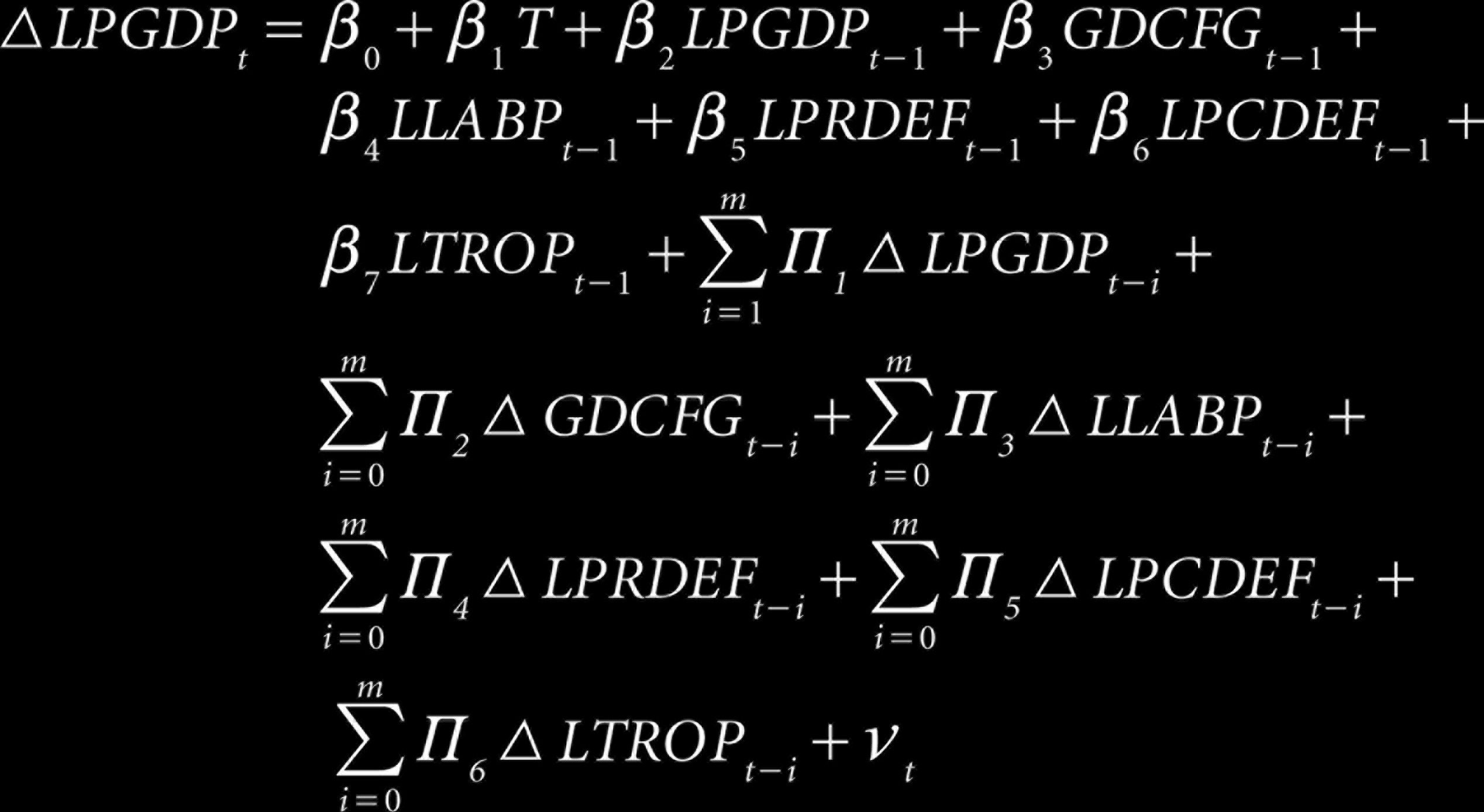
After the estimation of equations (4) and (5) by ordinary least square, the Wald test (F-statistic) was conducted to test for a long-run relationship. This test imposes a linear restriction on the coefficients of the one-period lagged level of variables, where the null hypothesis is no cointegration, and the alternative hypothesis is cointegration among the selected variables. The null and alternative hypotheses of these selected models are as follows:

For Equation (4)

H₀: α₂ = α₃ = α₄ = α₅ = α₆ = 0 (no long-run relationship)

H₁: α₂  0, α₃  0, α₄  0, α₅  α₆  0 (a long-run relationship exists)

For Equation (5)

H₀: β₂ = β₃ = β₄ = β₅ = β₆ = 0 (no long-run relationship)

H₁: β₂  0, β₃  0, β₄  0, β₅ β₆  β₇  0 (a long-run relationship exists)

Pesaran et al. (2001) have given lower- and upper-bound critical values of the F-statistics. The lower-bound critical value is based on the assumption that explanatory variables are integrated of order zero [I(0)], and the upper-bound critical value is integrated of order one [I(1)]. If the estimated F-value is smaller than the lower-bound critical value, then the null hypothesis of no long-run relationship is accepted, whereas, if the estimated F-statistic is higher than the upper- bound critical value, then the alternative hypothesis of a long-run relationship is accepted. However, if the estimated F-statistic falls in-between the lower- and upper-bound critical values, then the decision about cointegration is inconclusive.

After cointegration was confirmed, the long-run and short-run relationships were estimated using the following equations. The long-run equations are:

\begin{matrix} L P G D P_{t} = α_{0} + α_{1} T + \sum_{i = 1}^{m} α_{1} L P G D P_{t - i} + \sum_{i = 0}^{m} α_{2} G D C F G_{t - i} + \\ \sum_{i = 0}^{m} α_{3} L L A B P_{t - i} + \sum_{i = 0}^{m} α_{4} L P D E F_{t - i} + \\ \sum_{i = 0}^{m} α_{5} L T R O P_{t - i} + ε_{t} \end{matrix}

(6)

\begin{matrix} L P G D P_{t} = β_{0} + β_{1} T + \sum_{i = 1}^{m} β_{1} L P G D P_{t - i} + \sum_{i = 0}^{m} β_{2} G D C F G_{t - i} \\ + \sum_{i = 0}^{m} β_{3} L L A B P_{t - i} + \sum_{i = 0}^{m} β_{4} L P C D E F_{t - i} + \\ \sum_{i = 0}^{m} β_{5} L P R D E F_{t - i} + \sum_{i = 0}^{m} β_{6} L T R O P_{t - i} + v_{t} \end{matrix}

(7)

The following short-run dynamics of the parameters were estimated using error correction mechanisms:

\begin{matrix} △ L P G D P_{t} = α_{0} + \sum_{i = 1}^{m} Φ_{1} △ L P G D P_{t - i} + \sum_{i = 0}^{m} Φ_{2} △ G D C F G_{t - i} \\ + \sum_{i = 0}^{m} Φ_{3} △ L L A B P_{t - i} + \sum_{i = 0}^{m} Φ_{4} △ L P D E F_{t - i} + \end{matrix}

\sum_{i = 0}^{m} Φ_{5} △ L T R O P_{t - i} + ξ E C M_{t - 1} + ε_{t}

(8)

\begin{matrix} △ L P G D P_{t} = β_{0} + \sum_{i = 1}^{m} Π ​_{1}^{}_{​}^{} △ L P G D P_{t - i} + \sum_{i = 0}^{m} Π ​_{2} △ G D C F G_{t - i} \\ + \sum_{i = 0}^{m} Π ​_{3} △ L L A B P_{t - i} + \sum_{i = 0}^{m} Π ​_{4} △ L P R D E F_{t - i} \\ + \sum_{i = 0}^{m} Π ​_{5}^{}_{​}^{} △ L P C D E F_{t - i} + \sum_{i = 0}^{m} Π ​_{6} △ L T R O P_{t - i} \\ + ξ E C M_{t - 1} + v_{t} \end{matrix}

(9)

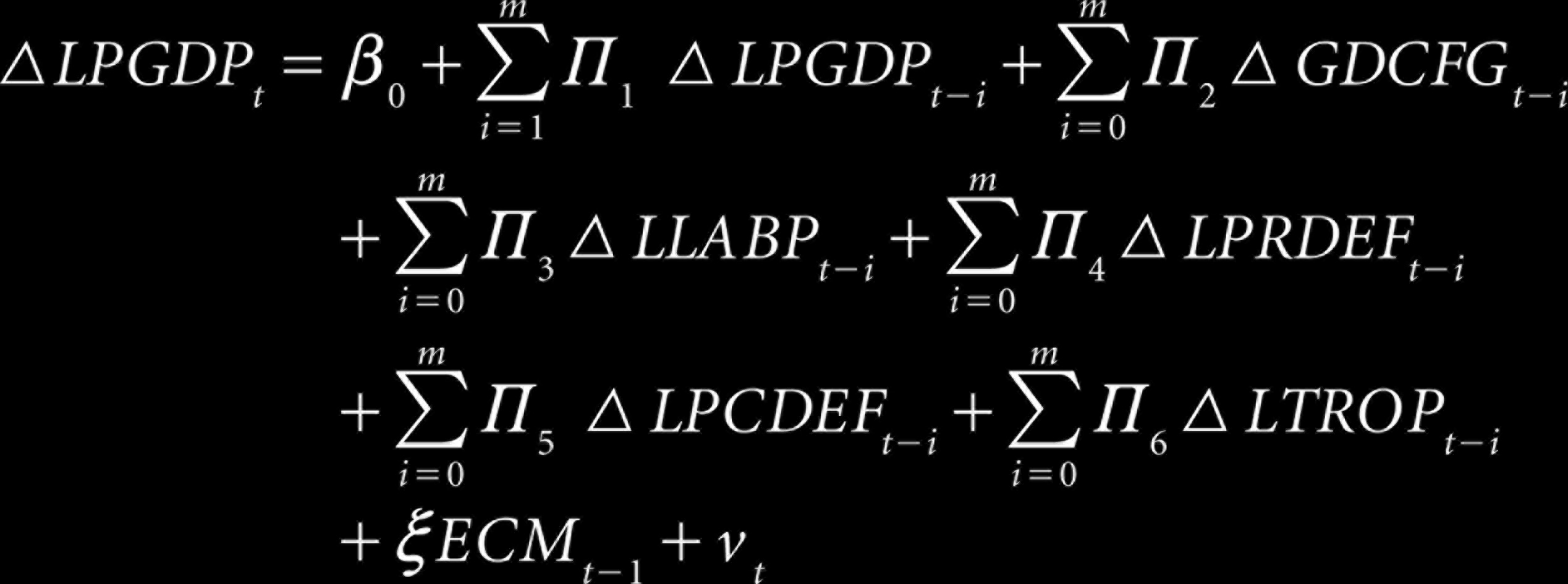
Where, T is a trend, Δ is the first difference operator, α₀ and β₀ are intercepts, Φ_i and Π_i are coefficients, ECM_t–1 is the one-period lagged error correction term, ξ is the speed of adjustment, ε_t and ν_t are error terms of the estimated models and all other variables are as defined before.

The next section analyses the trends in various types of defence spending during the selected period.

4. Analysis Of Trends In Defence Spending

India’s aggregate defence spending is divided into two major categories, that is, capital defence spending and revenue defence spending. Capital defence spending covers: the acquisition of land, construction works, infrastructure development, modernization and new weapon systems, aircrafts and aero engines, heavy and medium vehicles, other equipment, research and development, defence ordnance factories and others. Revenue defence spending is intended for day-to-day running expenses such as pay and allowances (salaries), pensions and miscellaneous expenses, transportation costs, maintenance works, repairs of machinery and equipment, stores, training costs and other related expenditure. Revenue defence spending is recurring in nature and does not create any capital assets, while capital defence spending is non--recurring and creates assets and is thus, more productive. More capital defence spending is necessary for India to become self-reliant in the production of defence equipment, which would also reduce the imports of arms and ammunition in future. However, both revenue and capital defence spending are required for maintaining a peaceful environment, which enhances economic growth by boosting confidence among investors.

The government spends a significant amount of its scarce resources on defence. Over the years, expenditure on defence and its major components (revenue and capital) has been rising (see Figure 2); the capital defence expenditure line is relatively flatter. Real defence expenditure has risen more than seven times over the last four decades. It would be very interesting to verify whether different types of defence spending have different impacts on the Indian economy.

Figure 2

Source: Handbook of Statistics on the Indian Economy, Reserve Bank of India. The base year is 2011–2012.

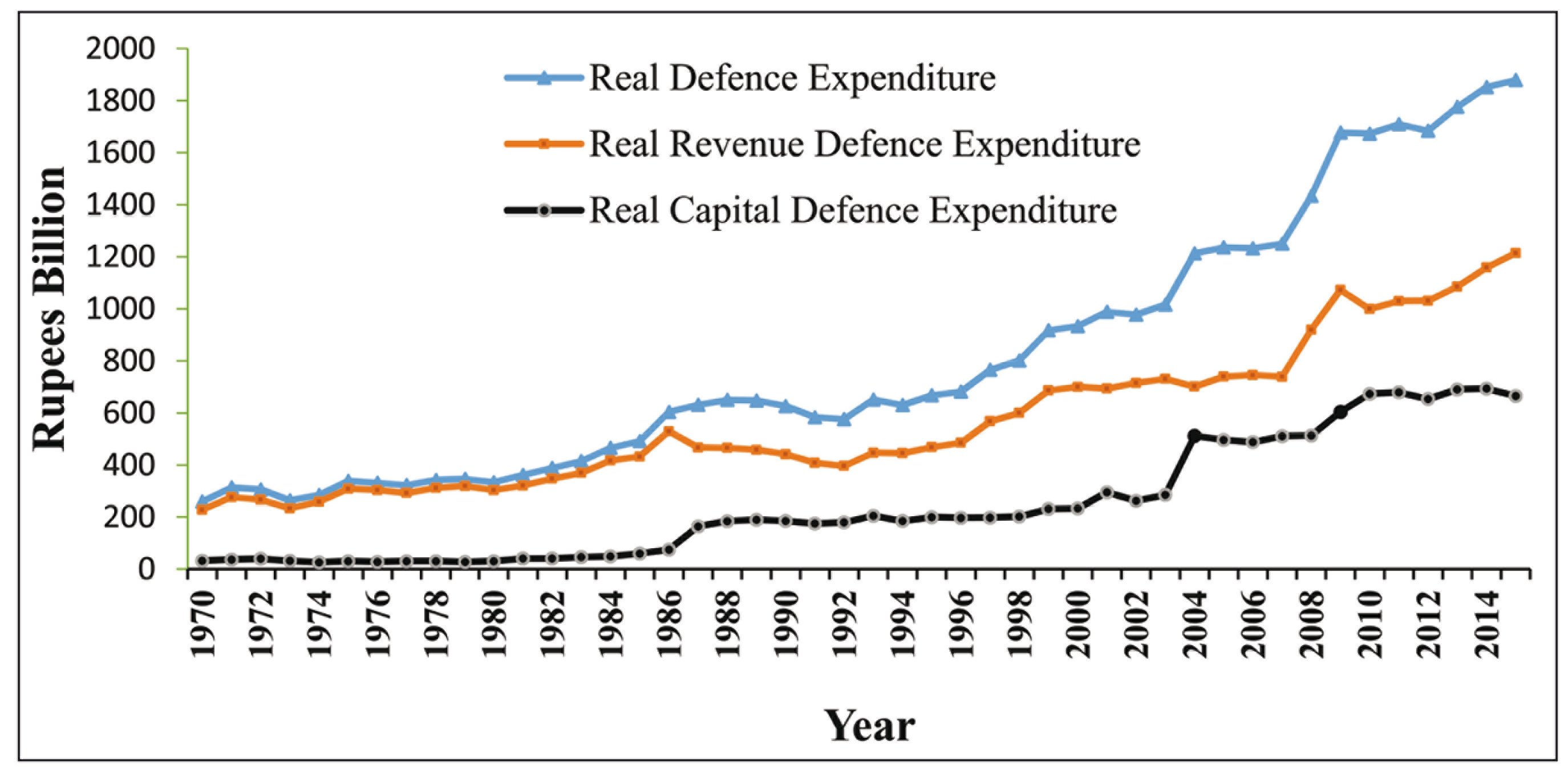
However, both defence and revenue defence expenditure as a percentage of GDP has been declined during the study period, especially from 1986 onwards (see Figure 3). Capital defence expenditure has slightly increased during the study period, but it was comparatively flatter than other types of defence expenditure. It is also seen that both per capita defence expenditure and per capita GDP have moved together with an increasing trend from 1970 to 2015 (see Figure 4). It is also verified that there exists a positive and strong co-relationship between GDP and the components of defence expenditure. Based on these preliminary findings of a strong co-relationship and co-movement between these variables, the study has tried to explore their relationship through advanced econometric analysis, presented in the following sections.

Figure 3

Source: Handbook of Statistics on the Indian Economy, Reserve Bank of India. The base year is 2011–2012.

Figure 4

Source: Handbook of Statistics on the Indian Economy, Reserve Bank of India.

5. Empirical Analysis

The empirical analysis is presented in this section. It includes the unit root tests for identifying the order of integration, bounds test for identifying cointegration among variables and finally, estimation of the long-run and short-run analyses.⁷

5.1 Identifying the Order of Integration

Table A1 (Appendix 1) shows the results of the unit root tests, where the null hypothesis assumes that the variable is non-stationary or has a unit root. Augmented Dickey–Fuller (ADF) and Phillips–Perron (PP) tests are applied to test the stationarity of these variables. The growth rate of GDCFG is stationary at the level, that is, I(0), whereas other variables like LPGDP, LLABP, LPDEF, LPRDEF, LPCDEF and LTROP are stationary at their first order only, that is, I(1). The mixture of I(0) and I(1) variables are an ideal precondition for applying the ARDL approach (Pesaran et al., 2001).

5.2 Bounds Testing Approaches for Cointegration

Tables A2 and A3 (Appendix 1) present the bounds test results for equations 4 and 5, respectively. The null hypothesis is of no long-run relationship among the selected variables. For model 1, the computed F-value (5.313) lies outside the upper-bound critical value at 1 per cent level of significance, thereby rejecting the null hypothesis and supports the existence of a long-run relationship. For the second model, the computed F-value is 4.672 and lies outside the upper-bound critical value at the 5 per cent significance level, thus accepting the alternative hypothesis of a long-run relationship. Therefore, these bounds test results confirm the cointegration relationship among the chosen models.

5.3 Estimation of the Long-run and Short-run Coefficients (Model 1)

The long-run and short-run coefficients of the selected ARDL models are presented in Table 1, where economic growth is used as the dependent variable, and the independent variables are capital, labour force, defence expenditure and trade openness. The lag length is selected by the Schwarz Bayesian criterion.

Table 1
Estimated Long-Run and Short-Run Coefficients using ARDL (Model 1)

Model: LPGDP = f (GDCFG, LLABP, LPDEF, LTROP)

Selected Model: ARDL (1, 0, 0, 0, 1) based on Schwarz Bayesian criterion

Long Run
Short Run

Variable Coeff S. E. p-values Variable Coeff S.E. p-values

GDCFG 0.004 0.001 0.02 ∆GDCFG 0.001* 0.001 0.00

LLABP –1.593* 0.257 0.00 ∆LLABP –0.580 0.235 0.02

LPDEF 0.191** 0.095 0.05 ∆LPDEF 0.069* 0.037 0.07

LTROP 0.222* 0.068 0.00 ∆LTROP –0.043 0.036 0.24

C 14.455* 1.532 0.00 C 0.009 0.003 0.01

TREND 0.024* 0.004 0.00 ECMTt–1 –0.364*** 0.114 0.00

Diagnostic Tests

Serial Correlation Test: 1.755 [0.188]

Normality Test: 1.350 [0.509]

Heteroscedasticity Test: 0.793 [0.598]

ARCH Test: 0.165 [0.687]

Ramsey RESET Test: 2.420 [0.129]

Model: LPGDP = f (GDCFG, LLABP, LPDEF, LTROP)
GDCFG	0.004**	0.001	0.02	∆GDCFG	0.001***	0.001	0.00
LLABP	–1.593***	0.257	0.00	∆LLABP	–0.580**	0.235	0.02
LPDEF	0.191**	0.095	0.05	∆LPDEF	0.069*	0.037	0.07
LTROP	0.222***	0.068	0.00	∆LTROP	–0.043	0.036	0.24
C	14.455***	1.532	0.00	C	0.009**	0.003	0.01
TREND	0.024***	0.004	0.00	ECMTt–1	–0.364***	0.114	0.00
Diagnostic Tests
Serial Correlation Test:	1.755 [0.188]
Normality Test:	1.350 [0.509]
Heteroscedasticity Test:	0.793 [0.598]
ARCH Test:	0.165 [0.687]
Ramsey RESET Test:	2.420 [0.129]

Source: Authors’ estimations.

Notes: ***, ** and * denote 1, 5 and 10 per cent levels of significance, respectively. Coeff and S.E. refer to the coefficients and standard errors, respectively. Figures in parentheses are P-values. ARDL: Autoregressive distributed lag. ARCH Test: Autoregressive conditional heteroscedastic test. Ramsey RESET Test: Ramsey regression equation specification error test.

The long-run results revealed that defence expenditure has a positive and significant effect on economic growth in India at the 5 per cent significance level. Due to persistent cross-border problems with its neighbouring countries, especially Pakistan and China, and to control other internal problems such as Naxalism, terrorism and internal security, the Indian government has been strengthening its defence sector over the years. For example, in 2015, more than ₹2,258 billion was allocated to defence.

It is also seen from section 3 that defence expenditure has risen in line with GDP. When the growth rate of GDP has risen, defence expenditure also has risen, especially after the reform period. A high positive co-relationship between defence expenditure and GDP during the study period also supports this positive impact of defence expenditure on economic growth. Similar kinds of findings are found in Benoit (1978), Dunne et al. (2001, 2005), Kollias et al. (2004) and Smith and Dunne (2001). The results also confirm that defence spending has a positive impact on economic growth in the short run at 10 per cent significance level. Therefore, defence expenditure can enhance national income in India in both the long run and short run. The elasticity of labour force participation is significant at 1 per cent level and adversely affects the national output in the long run, contrary to standard economic theory. This could be because of the abundant unskilled labour force in India. With structural transformation, India’s current economic growth has been mainly contributed by the service sector, which requires a skilled workforce, therefore, the large unskilled workforce has an adverse effect on economic growth. Capital formation positively affects economic growth in the long run and short run, as expected. However, trade openness affects economic growth in the long run but does not significantly affect output growth in the short run. The coefficient of the error correction term is negative and significant at 1 per cent level, indicating that the speed of convergence is 36.4 per cent.

5.4 How Robust Were Our Results?

5.4.1 Does Capital and Revenue Defence Spending Affect Economic Growth?

To check for robustness, model (1) was re-estimated by segregating defence expenditure into defence revenue expenditure and defence capital expenditure, keeping the other variables as before. The results of model (2) are presented in Table 2. The primary purpose was to examine the differential impact of both revenue and capital defence expenditure on economic growth.

Table 2
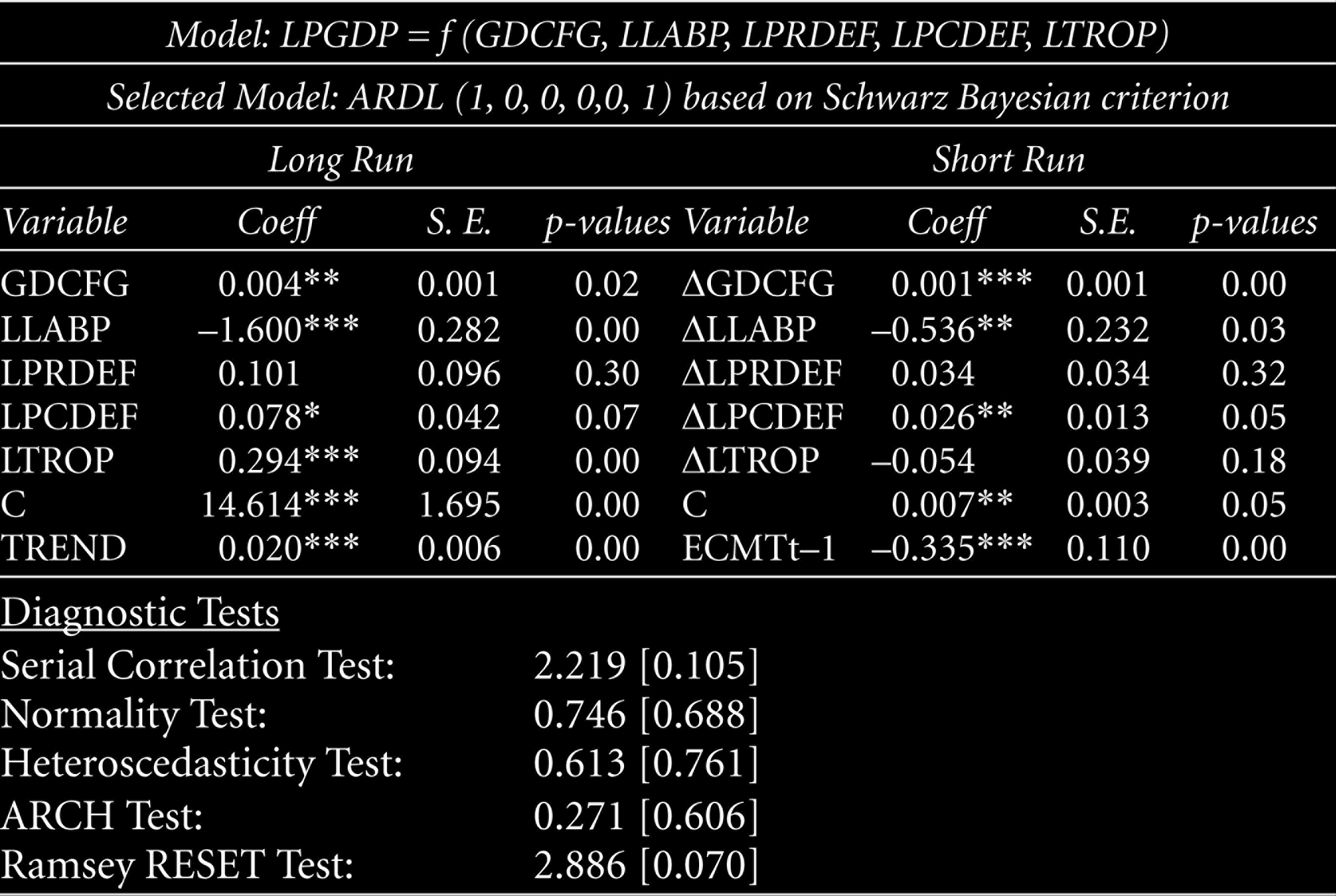
Estimation of Long-Run and Short-Run Coefficients Using ARDL (Model 2)

Model: LPGDP = f (GDCFG, LLABP, LPRDEF, LPCDEF, LTROP)

Selected Model: ARDL (1, 0, 0, 0,0, 1) based on Schwarz Bayesian criterion

Long Run
Short Run

Variable Coeff S. E. p-values Variable Coeff S.E. p-values

GDCFG 0.004 0.001 0.02 ∆GDCFG 0.001* 0.001 0.00

LLABP –1.600* 0.282 0.00 ∆LLABP –0.536 0.232 0.03

LPRDEF 0.101 0.096 0.30 ∆LPRDEF 0.034 0.034 0.32

LPCDEF 0.078* 0.042 0.07 ∆LPCDEF 0.026 0.013 0.05

LTROP 0.294* 0.094 0.00 ∆LTROP –0.054 0.039 0.18

C 14.614* 1.695 0.00 C 0.007 0.003 0.05

TREND 0.020* 0.006 0.00 ECMTt–1 –0.335* 0.110 0.00

Diagnostic Tests

Serial Correlation Test: 2.219 [0.105]

Normality Test: 0.746 [0.688]

Heteroscedasticity Test: 0.613 [0.761]

ARCH Test: 0.271 [0.606]

Ramsey RESET Test: 2.886 [0.070]

Model: LPGDP = f (GDCFG, LLABP, LPRDEF, LPCDEF, LTROP)
GDCFG	0.004**	0.001	0.02	∆GDCFG	0.001***	0.001	0.00
LLABP	–1.600***	0.282	0.00	∆LLABP	–0.536**	0.232	0.03
LPRDEF	0.101	0.096	0.30	∆LPRDEF	0.034	0.034	0.32
LPCDEF	0.078*	0.042	0.07	∆LPCDEF	0.026**	0.013	0.05
LTROP	0.294***	0.094	0.00	∆LTROP	–0.054	0.039	0.18
C	14.614***	1.695	0.00	C	0.007**	0.003	0.05
TREND	0.020***	0.006	0.00	ECMTt–1	–0.335***	0.110	0.00
Diagnostic Tests
Serial Correlation Test:	2.219 [0.105]
Normality Test:	0.746 [0.688]
Heteroscedasticity Test:	0.613 [0.761]
ARCH Test:	0.271 [0.606]
Ramsey RESET Test:	2.886 [0.070]

Source: Authors’ estimations.

Notes: ***, ** and * denote 1, 5 and 10 per cent levels of significance, respectively. Coeff and S.E. refer to coefficients and standard errors, respectively. Figures in parentheses are P-values. ARDL: Autoregressive distributed lag. ARCH Test: Autoregressive conditional heteroscedastic test. Ramsey RESET Test: Ramsey regression equation specification error test.

The findings reveal that revenue defence expenditure does not affect economic growth in the long run or in the short run. However, the coefficients of capital defence expenditure are positive and significant at 5 per cent and 10 per cent levels in the short run and long run, respectively, indicating that more resources should be devoted to capital defence spending rather than to revenue defence spending. This is the significant contribution of our study towards public policy in defence spending in India. The coefficients of the other variables are similar to the previous model. The elasticity of labour force participation has an adverse impact on economic growth both in the short and long run, and as before, capital formation positively influences economic growth. Finally, the elasticity of trade openness has a positive and significant influence on economic growth in the long run but an insignificant effect in the short run. Thus, trade openness plays a vital role in the long run rather than in the short run. The rate of convergence is –0.33; all of these are similar to the previously estimated model.

5.5 Diagnostic Tests and Stability Test of the ARDL Models

The diagnostic test and stability test of the selected ARDL models are presented in two phases. The first phase presents all the post-estimation results for both models 1 and 2, like serial correlation, normality test, heteroscedasticity test, autoregressive conditional heteroscedastic test and the Ramsey Regression Equation Specification Error Test. In the second phase, the study examined the stability tests of the model using the cumulative sum (CUSUM) and the cumulative sum of squares (CUSUM SQ) tests. The results of the diagnostic test results show that the estimated models have passed all the diagnostic tests (the lower part of Tables 1 and 2 for models 1 and 2, respectively). Furthermore, the results of the stability tests show that neither the CUSUM nor the CUSUM SQ statistics exceed the bounds of 5 per cent significance level, which confirms that the estimated models are stable over time (Figures A1 and A2, see Appendix).

5.6 Is There Any Causality Between Defence Expenditure and Economic Growth?

The significance of the error correction terms in the above-estimated equations conveys information on the Granger causality among the variables. The direction of the causality is not clear, and it would be interesting to know whether it is unidirectional or bidirectional.

Therefore, the article examined the causality between economic growth and defence expenditure by using a modified version of the Granger causality test proposed by Toda and Yamamoto (1995). The test is valid regardless of whether a series is I(0), I(1) or I(2) and also whether these series are cointegrated or not-cointegrated. This approach fits a standard vector autoregressive model in the levels of the variables, irrespective of their level of integration. Thus, the risk associated with the possibility of wrongly identifying the integration order of the series is minimised. The first step is to determine the order of integration (d_max) of the series under consideration and the optimal lag, k. Then a (k + d_max) order of Vector autoregression (VAR) is estimated, and the coefficients of the last lagged d_max vector are ignored. The application of the Toda and Yamamoto (1995) procedure ensures that the usual test statistic for Granger causality has the standard asymptotic distribution, where valid inferences can be made.

To carry out the above-modified version of the Granger causality test, we represent the economic growth-defence expenditure models in the following VAR system:⁸

5.6.1 Between Economic Growth and Defence Expenditure

\begin{matrix} L P G D P_{t} = α_{0} + \sum_{i = 1}^{k} α_{1} L P G D P_{t - i} + \sum_{i = k + 1}^{d_{\max}} α_{2} L P G D P_{t - i} + \\ \sum_{i = 1}^{k} Φ_{1} L P D E F_{t - i} + \sum_{i = k + 1}^{d_{\max}} Φ_{2} L P D E F_{t - i} + λ_{1 t} \end{matrix}

(10)

\begin{matrix} L P D E F_{t} = β_{0} + \sum_{i = 1}^{k} β_{1} L P D E F_{t - i} + \sum_{i = k + 1}^{d_{\max}} β_{2} L P D E F_{t - i} + \\ \sum_{i = 1}^{k} δ_{1} L P G D P_{t - i} + \sum_{i = k + 1}^{d_{\max}} δ_{2} L P G D P_{t - i} + λ_{2 t} \end{matrix}

(11)

5.6.2 Between Economic Growth and Capital Defence Expenditure

\begin{matrix} L P G D P_{t} = α_{0} + \sum_{i = 1}^{k} α_{1} L P G D P_{t - i} + \sum_{i = k + 1}^{d_{\max}} α_{2} L P G D P_{t - i} + \\ \sum_{i = 1}^{k} Φ_{1} L P C D E F_{t - i} + \sum_{i = k + 1}^{d_{\max}} Φ_{2} L P C D E F_{t - i} + λ_{1 t} \end{matrix}

(12)

\begin{matrix} L P C D E F_{t} = β_{0} + \sum_{i = 1}^{k} β_{1} L P C D E F_{t - i} + \sum_{i = k + 1}^{d_{\max}} β_{2} L P C D E F_{t - i} + \\ \sum_{i = 1}^{k} δ_{1} L P G D P_{t - i} + \sum_{i = k + 1}^{d_{\max}} δ_{2} L P G D P_{t - i} + λ_{2 t} \end{matrix}

(13)

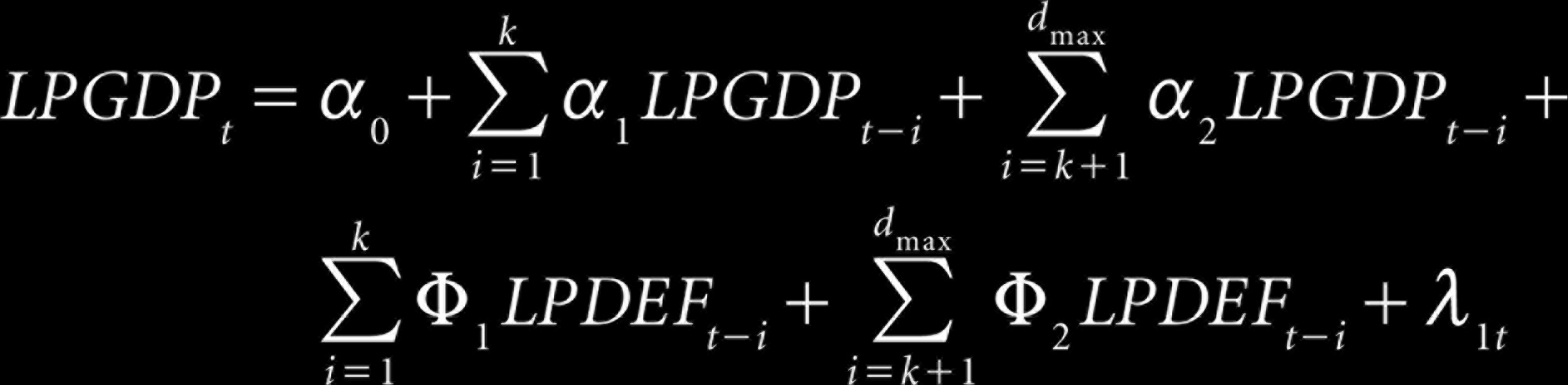
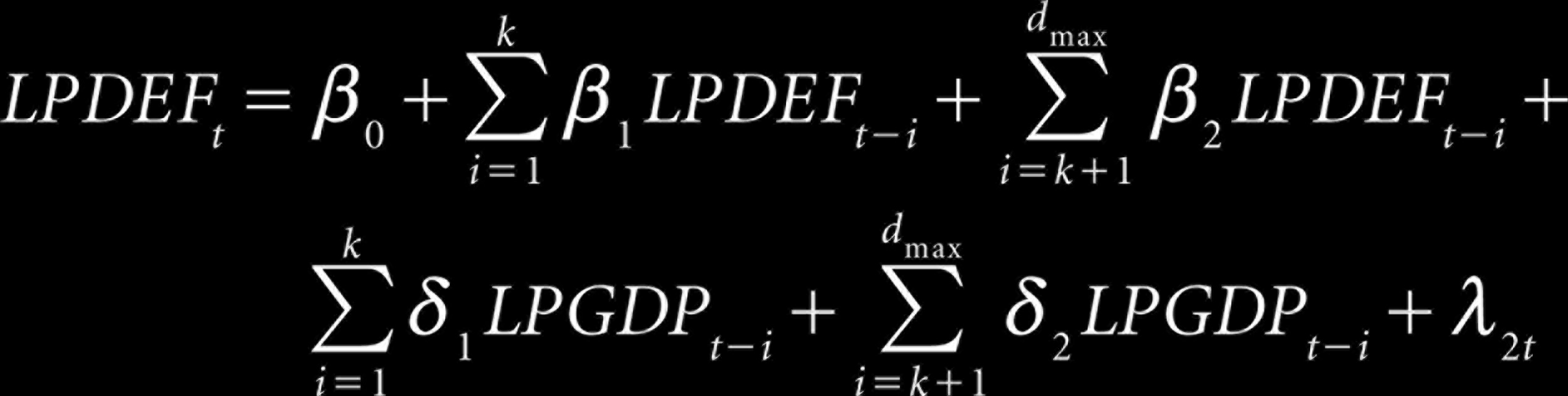
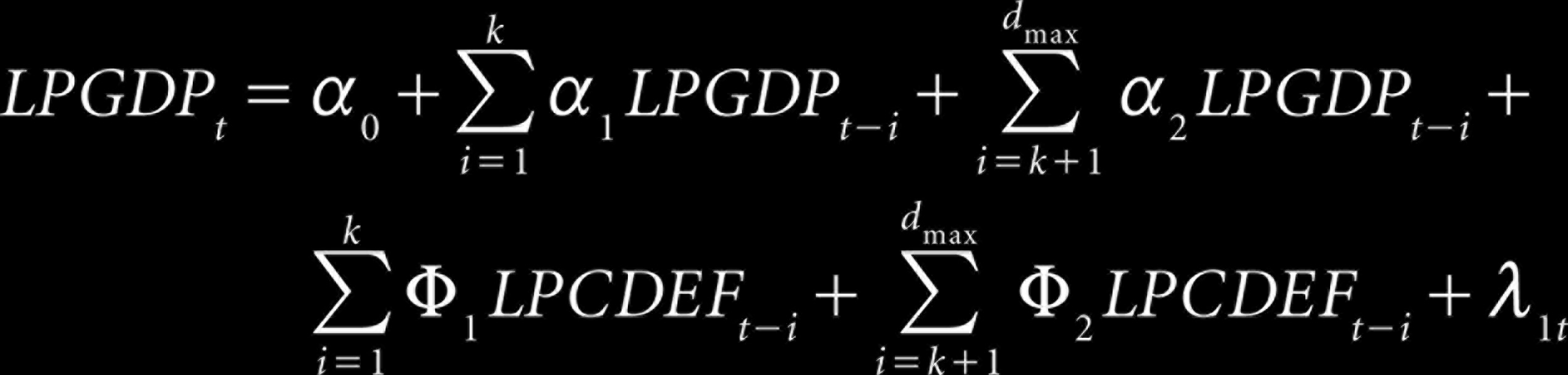
where the variables are defined earlier.

From equation (10), Granger causality from LPDEF_t to LPGDP_t implies Φ_1i = 06_i; similarly, in equation (11), LPGDP_t Granger causes LPDEF_t, if δ_1i = 06_i. A similar type of analysis is carried out between economic growth and per capita capital defence expenditure. To test this, we have modified equations (10) and (11) by replacing LPDEF with LPCDEF. The results of the causality tests are presented in Table 3 by using the Akaike Information Criteria.

Table 3

Results of The Toda-Yamamoto Approach to Granger Causality Test

Variables	Statistics (Chi-sq.)	Direction of causality
LPDEF does not Granger Cause LPGDP	23.87*** (0.00)	Bidirectional
LPGDP does not Granger Cause LPDEF	12.59** (0.05)	(LPDEF↔LPGDP)
LPCDEF does not Granger Cause LPGDP	17.56*** (0.00)	Unidirectional
LPGDP does not Granger Cause LPCDEF	1.58 (0.95)	(LPCDEF→LPGDP)

Source: Authors’ estimations.

Note: ** and *** indicate significance at the 5 per cent and 1 per cent levels, respectively.

The causality test results show that the hypothesis of per capita defence expenditure does not Granger cause per capita GDP, and per capita GDP does not Granger cause per capita defence expenditure, which is rejected by the applied causality test. Therefore, a bidirectional causality is found between defence expenditure and economic growth. However, while testing causality between economic growth and capital defence expenditure, we found that causality runs one way from capital defence expenditure to economic growth and not the reverse. A bidirectional causality has been found for Asia, Europe, Latin America and the Caribbean and the Middle East and North Africa, but no causality has been found for upper-middle income European, Central Asian and Sub-Saharan African countries (Chen, Lee, & Chiu, 2014). Lai, Huang, and Yang (2005) also found a casualty from defence expenditure to income for China. Thus, more resources should be diverted towards capital defence expenditure to enhancing the economic growth of the Indian economy.

6. Conclusion And Policy Implications

Defence expenditure is a significant element of fiscal strategy aimed at ensuring the strength and stability of an economy. In a developing country like India, it is especially interesting to investigate whether an increase in defence spending boosts or hinders economic growth. The motivation for studying the nexus between growth and defence spending in India is also based on country-specific features, like its cross-border problems with its neighbouring countries, especially Pakistan and China, and various internal issues such as Naxalism, terrorism and insurgency, ensuring internal security and integrity and peace in the country. Country-specific studies on India on these issues are very few.

Thus, this study investigates the impact of defence spending on economic growth in India from 1970–1971 to 2015–2016 by utilising the ARDL and Toda-Yamamoto Granger Causality approaches. It also examines the differential impact of both revenue and capital defence expenditure on economic growth.

The empirical analysis shows that defence expenditure positively affects economic growth both in the long run and short run. Further, while capital defence spending has a positive and significant effect on economic growth in both the short run and the long run, revenue defence expenditure does not have any significant effect in the long run and short run. It also finds that capital formation positively influences economic growth in India and that trade openness plays a vital role in the long run rather than in the shortrun. The application of the Toda and Yamamoto (1995) Granger causality test finds a bidirectional causality between defence expenditure and economic growth, but a unidirectional causality from capital defence expenditure to economic growth and not the reverse. These findings could help policy makers frame a suitable policy for the Indian defence sector.

In recent years, India’s defence spending as a share of its GDP has been comparatively lower (less than 1.7 per cent in 2015–2016)⁹ than spending in Pakistan and China. Overall, defence expenditure should be enhanced to manage the country’s internal security and heightening tensions with its neighbours. The provision of a peaceful economic and political environment would induce higher domestic and foreign investment, which in turn contributes to economic growth. The share of India’s capital defence spending in GDP, particularly, is very low (less than 0.7 per cent) and constitutes just one-third of total defence spending. Thus, spending on modernising the equipment and the acquisition of technology is required to enable the country to tackle the increasing threats and challenges to national security.

The findings of the study suggest for restructuring the composition of India’s defence spending in favour of greater capital defence spending (without a reduction in revenue defence spending, which is necessary for the smooth functioning of the sector). Overall, what is needed is a far larger allocation of resources to defence spending, especially capital defence spending, to enhance economic growth of the Indian economy.

Footnotes

Acknowledgements

The authors would like to thank the editor and the anonymous referees for their comments which have substantially improved the quality of the paper. Any error and omission in the paper are the authors’ alone.

Declaration of Conflicting Interests

The authors declared no potential conflicts of interest with respect to the research, authorship and/or publication of this article.

Funding

The authors received no financial support for the research, authorship and/or publication of this article.

Appendix 1

Table A3

Results of the ARDL Bound Test Model (2)

Model 2: LPGDP = f(GDCFG, LLABP, LPRDEF, LPCDEF, LTROP)
ARDL Bound Test: F-statistic: 4.672***
Critical Value Bounds
Significance	Lower-Bound I(0)	Upper-Bound I(1)
10%	2.26	3.35
5%	2.62	3.79
1%	3.41	4.68

Source: Authors’ estimations.

Notes: ARDL: Autoregressive distributed lag.

Descriptive Statistics

Table A4 presents the summary statistics of the selected variables used in the analysis. The highest and lowest mean is found for LPGDP and LTROP, respectively. However, the results of the standard deviation show that less volatility is observed in LLABP, whereas, high volatility does exist in capital formation (GDCFG).

Notes

References

Abu-Bader

, & Abu-Qarn

A. S.

(2003). Government expenditures, military spending and economic growth: Causality evidence from Egypt, Israel, and Syria. Journal of Policy Modeling, 25(6–7), 567–583.

Agenor

P. R.

, & Neanidis

K. C.

(2011). The allocation of public expenditure and economic growth. The Manchester School, 79(4), 899–931.

Alexander

W. R. J.

(1990). The impact of defence spending on economic growth: A multi‐sectoral approach to defence spending and economic growth with evidence from developed economies. Defence and Peace Economics, 2(1), 39–55.

Atesoglu

H. S.

(2002). Defence spending promotes aggregate output in the United States: Evidence from cointegration analysis. Defence and Peace Economics, 13(1), 55–60.

Benoit

(1978). Growth and defence in developing countries. Economic Development and Cultural Change, 26(2), 271–280.

Chen

P. F.

, Lee

C. C.

, & Chiu

Y. B.

(2014). The nexus between defence expenditure and economic growth: New global evidence. Economic Modelling, 36, 474–483.

Chowdhury

A. R.

(1991). A causal analysis of defence spending and economic growth. Journal of Conflict Resolution, 35(1), 80–97.

Dakurah

A. H.

, Davies

S. P.

, & Sampath

R. K.

(2001). Defence spending and economic growth in developing countries: A causality analysis. Journal of Policy Modeling, 23(6), 651–658.

Deger

(1986). Economic development and defence expenditure. Economic Development and Culture Change, 35(1), 179–196.

10.

Deger

, & Sen

(1983). Military expenditure, spin-off and economic development. Journal of Development Economics, 13(1–2), 67–83.

11.

Deger

, & Smith

(1983). Military expenditure and growth in LDCs. Journal of Conflict Resolution, 27(2), 335–353.

12.

DeGrasse

R. W.

(2016). Military expansion, economic decline: The impact of military spending on US economic performance. New York, USA: Routledge.

13.

Devarajan

, Swaroop

, & Zou

(1996). The composition of public expenditure and economic growth. Journal of Monetary Economics, 37(2), 313–344.

14.

Dritsakis

(2004). Defense spending and economic growth: An empirical investigation for Greece and Turkey. Journal of Policy Modeling, 26(2), 249–264.

15.

Dunne

, Nikolaidou

, & Vougas

(2001). Defence spending and economic growth: A causal analysis for Greece and Turkey. Defence and Peace Economics, 12(1), 5–26.

16.

Dunne

J. P.

, Smith

R. P.

, & Willenbockel

(2005). Models of military expenditure and growth: A critical review. Defence and Peace Economics, 16, 449–461.

17.

Edwards

(1992). Trade orientation, distortions, and growth in developing countries. Journal of Development Economics, 39(1), 31–57.

18.

Kollias

, Manolas

, & Paleologou

S. M.

(2004). Defence expenditure and economic growth in the European Union: A causality analysis. Journal of Policy Modeling, 26(5), 553–569.

19.

Faini

, Annez

, & Taylor

(1984). Defence spending, economic structure, and growth: Evidence among countries and over time. Economic Development and Culture Change, 32(3), 487–498.

20.

Farrar

D. E.

, & Glauber

R. R.

(1967). Multicollinearity in regression analysis: The problem revisited. The Review of Economic and Statistics, 49(1), 92–107.

21.

Galvin

(2003). The impact of defence spending on the economic growth of developing countries: A cross-section study. Defence and Peace Economics, 14(1), 51–59.

22.

Joerding

(1986). Economic growth and defence spending: Granger causality. Journal of Development Economics, 21(1), 35–40.

23.

Jones

L. E.

, Manuelli

R. E.

, & Rossi

P. E.

(1993). Optimal taxation in models of endogenous growth. Journal of Political Economy, 101(3), 485–517.

24.

Kentor

, & Kick

(2008). Bringing the military back in: Military expenditures and economic growth, 1990 to 2003. Journal of World-Systems Research, 14(2), 142–172.

25.

Klein

(2004). Military expenditure and economic growth: Peru 1970–1996. Defence and Peace Economics, 15(3), 275–288.

26.

Lai

C. N.

, Huang

B. N.

, & Yang

C. W.

(2005). Defence spending and economic growth across the Taiwan Straits: A threshold regression model. Defence and Peace Economics, 16(1), 45–57.

27.

Lipow

, & Antinori

C. M.

(1995). External security threats, defence expenditures, and the economic growth of less-developed countries. Journal of Policy Modeling, 17(6), 579–595.

28.

Mansfield

E. R.

, & Helms

B. P.

(1982). Detecting multicollinearity. The American Statistician, 36(3a), 158–160.

29.

Mintz

, & Huang

(1990). Defence expenditures, economic growth, and the peace dividend. American Political Science Review, 84(4), 1283–1293.

30.

Perlo-Freeman

, Fleurant

, Wezeman

P. D.

, & Wezeman

S. T.

(2015). Trends in world military expenditure, 2014. Stockholm International Peace Research Institute (SIPRI) Fact Sheet, Sweden, April 2015.

31.

Pesaran

M. H.

, Shin

, & Smith

R. J.

(2001). Bounds testing approaches to the analysis of level relationships. Journal of Applied Econometrics, 16(3), 289–326.

32.

Pieroni

, d’Agostino

, & Lorusso

(2008). Can we declare military Keynesianism dead? Journal of Policy Modeling, 30(5), 675–691.

33.

Rasler

, & Thompson

W. R.

(1998). Defence burdens, capital formation, and economic growth. Journal of Conflict Resolution, 32(1), 61–86.

34.

Sinha

, & Sinha

(2002). Openness, investment and economic growth in Asia. The Indian Economic Journal, 49(4), 90–95.

35.

Smith

, & Dunne

(2001). Military expenditure growth and investment. Abril: Birbeck College and Middlesex University Business School.

36.

Stokey

N. L.

, & Rebelo

(1995). Growth effects of flat-rate taxes. Journal of Political Economy, 103, 519–550.

37.

Tian

, Fleurant

, Wezeman

P. D.

, & Wezeman

S. T.

(2017). Trends in world military expenditure, 2016. Stockholm International Peace Research Institute (SIPRI) Fact Sheet, April 2017.

38.

Toda

H. Y.

, & Yamamoto

(1995). Statistical inference in vector autoregressions with the possibly integrated process. Journal of Econometrics, 66(1–2), 225–250.

39.

Ward

M. D.

, Davis

, Penubarti

, Rajmaira

, & Cochran

(1991). Country survey I –Military spending in India. Defence and Peace Economics, 3(1), 41–63.

40.

Yang

, Hong

, Jung

, & Lee

J. D.

(2015). Arms or butter: The economic effect of an increase in military expenditure. Journal of Policy Modeling, 37(4), 596–615.

41.

Yildirim

, Sezgin

, & Öcal

(2005). Military expenditure and economic growth in Middle Eastern countries: A dynamic panel data analysis. Defence and Peace Economics, 16(4), 283–295.

42.

Ynikkaya

(2003). Trade openness and economic growth: A cross-country empirical investigation. Journal of Development Economics, 72(1), 57–89.

Model: LPGDP = f (GDCFG, LLABP, LPDEF, LTROP)
Selected Model: ARDL (1, 0, 0, 0, 1) based on Schwarz Bayesian criterion
Long Run				Short Run
Variable	Coeff	S. E.	p-values	Variable	Coeff	S.E.	p-values
GDCFG	0.004**	0.001	0.02	∆GDCFG	0.001***	0.001	0.00
LLABP	–1.593***	0.257	0.00	∆LLABP	–0.580**	0.235	0.02
LPDEF	0.191**	0.095	0.05	∆LPDEF	0.069*	0.037	0.07
LTROP	0.222***	0.068	0.00	∆LTROP	–0.043	0.036	0.24
C	14.455***	1.532	0.00	C	0.009**	0.003	0.01
TREND	0.024***	0.004	0.00	ECMTt–1	–0.364***	0.114	0.00
Diagnostic Tests
Serial Correlation Test:			1.755 [0.188]
Normality Test:			1.350 [0.509]
Heteroscedasticity Test:			0.793 [0.598]
ARCH Test:			0.165 [0.687]
Ramsey RESET Test:			2.420 [0.129]

Model: LPGDP = f (GDCFG, LLABP, LPRDEF, LPCDEF, LTROP)
Selected Model: ARDL (1, 0, 0, 0,0, 1) based on Schwarz Bayesian criterion
Long Run				Short Run
Variable	Coeff	S. E.	p-values	Variable	Coeff	S.E.	p-values
GDCFG	0.004**	0.001	0.02	∆GDCFG	0.001***	0.001	0.00
LLABP	–1.600***	0.282	0.00	∆LLABP	–0.536**	0.232	0.03
LPRDEF	0.101	0.096	0.30	∆LPRDEF	0.034	0.034	0.32
LPCDEF	0.078*	0.042	0.07	∆LPCDEF	0.026**	0.013	0.05
LTROP	0.294***	0.094	0.00	∆LTROP	–0.054	0.039	0.18
C	14.614***	1.695	0.00	C	0.007**	0.003	0.05
TREND	0.020***	0.006	0.00	ECMTt–1	–0.335***	0.110	0.00
Diagnostic Tests
Serial Correlation Test:			2.219 [0.105]
Normality Test:			0.746 [0.688]
Heteroscedasticity Test:			0.613 [0.761]
ARCH Test:			0.271 [0.606]
Ramsey RESET Test:			2.886 [0.070]