Technology Shocks and Non-stationary Hours in Emerging Countries and DSVAR

Abstract

We test a standard DSGE (Dynamic Stochastic General Equilibrium) model on impulse responses of hours worked and real GDP after technology and non-technology shocks in emerging market economies (EMEs). Most dynamic macroeconomic models assume that hours worked are stationary. However, in the data, we observe apparent changes in hours worked from 1970 to 2013 in these economies. Motivated by this fact, we first estimate a structural vector autoregression (SVAR) model with a specification of hours in difference (DSVAR) and then set up a DSGE model by incorporating permanent labour supply (LS) shocks that can generate a unit root in hours worked, while preserving the property of a balanced growth path. These LS shocks could be associated with very dramatic changes in LS which look permanent in these economies. Hence, the identification restriction in our models comes from the fact that both technology and LS shocks have a permanent effect on GDP yet only the latter shocks have a long-run impact on hours worked. For inference purposes, we compare empirical impulse responses based on the EMEs data to impulse responses from DSVARs run on the simulated data from the model. The results show that a DSGE model with permanent LS shocks that can generate a unit root in hours worked is required to properly evaluate the DSVAR in EMEs as this model is able to replicate indirectly impulse responses obtained from a DSVAR on the actual data.

JEL Classification: C32, E32

Keywords

Non-stationary Hours DSGE Models DSVAR Approach

1. Introduction

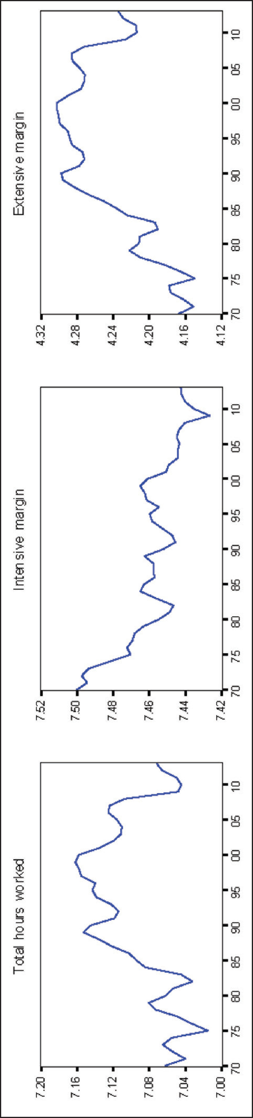
Many dynamic macroeconomic models should be able to match data across all frequencies since they have generated business cycle fluctuations as well as long-run growth paths. Around this path output, consumption and investment grow at the same rate while great ratios (such as consumption-to-output ratio) and hours are stationary (see King, Plosser, & Rebelo, 1998). However, the data clearly show that hours worked per capita are highly persistent and non-stationary during the past four decades in emerging market economies (EMEs) which are shaped by both extensive and intensive margins but it is apparent that it is mostly shaped by movements in the extensive margin (see Figure 1). Then, these models are not able to reproduce impulse response functions (IRFs) obtained from empirical models in EMEs such as VARs (Vector autoregression). In this paper, we identify mechanism that enables a standard DSGE model to fit non-stationary hours worked data in EMEs, while preserving the property of a balance growth path and then test this model on impulse responses of hours worked and real GDP after technology and non-technology shocks in these economies.

Motivated by these facts and the patterns observed in the data used for this study, we first estimate a structural vector autoregression (SVAR) model with a specification of hours in difference (DSVAR) from 1970 to 2013 and then build a DSGE model in which hours have a stochastic trend, including two permanent shocks. In addition to a permanent technology shock, the model includes labour supply (LS) shocks which yield non-stationary hours as in Chang, Doh, and Schorfheide (2006). One of the reasons hours could be non-stationary is because there might be a LS shock in these economies. Our research suggests that these LS shocks could be associated with very dramatic changes in LS which look permanent following changes in demographic structure, in home and market production and in labour market participation, especially in female labour participation (see Section 2).

Regarding the theoretical model, we impose long-run restrictions (Blanchard & Quah, 1989) to identify structural VARs and then compute the impulse responses of hours and real GDP for each emerging country. The identification restriction comes from the fact that both technology and LS shocks have a permanent effect on GDP yet only the LS shocks have a permanent impact on the hours worked. We have some degree of confidence that our model accurately reflects basic features of these economies because the restriction on the DSGE and the DSVAR are consistent with the pattern of long-run growth in emerging economies. In addition, the consumption-to-output ratio seems to be balanced in these economies. Hence, it cannot be that technology shocks derive non-stationary hours.¹ The way we test the implications of the model is to compare the empirical IRFs with those obtained from running an identical DSVAR on model generated data of the same length as the actual data. The literature calls this as Sims-Cogley-Nason approach because it has been advocated by Sims (1980) and applied by Cogley and Nason (1995). It involves treating the data from the actual economy and model economy symmetrically.

Figure 1

Notes: The figure displays the fluctuations of total hours worked, intensive and extensive margins for the period 1970–2013. Note that the first figures represent total hours worked (e.g. Brazil); second figures display intensive margin (e.g. Brazil1) and third figures represent extensive margin (e.g. Brazil2). All variables are in per capita terms and are logged.

Under these identification restrictions and this economic interpretation, LS and technology shocks seem to have a positive permanent impact on GDP in almost all EMEs. Moreover, a technology shock does not have any long-run impact on hours (by assumption) as it temporarily declines after a technology shock in Brazil, Hungary and Turkey. However, for Chile, Colombia, Mexico, Peru, Sri Lanka, South Africa and Thailand, a technology shock increases the hours worked. Besides, a LS shock has a positive long-run impact on hours worked for all these economies although it is not significant. To ensure that the VAR procedure works well, the consumption-to-output ratio (C/Y) is added. Augmenting the specification with an additional variable does not change the results much in most cases. However, the results appear more significant when compared with the two-variable VAR models.

We then estimate a DSVAR model on simulated data from the DSGE model and compute the IRFs of hours and real GDP to technology and LS shocks using long-run restrictions. We observe that hours worked increases permanently after a positive LS shock but it decreases temporarily after a positive technology shock. Moreover, real GDP rises permanently after a positive technology shock but following a positive LS shock it decreases in the beginning of the period and then rises permanently. Our results show that the VAR is not able to capture the significant impulse responses of the benchmark model. For robustness, we first build a production technology with the permanent labour-augmenting productivity shock which represents the cumulative product of ‘growth shocks’ (see Aguiar & Gopinath, 2007). We then build a DSGE model with a productivity technology shock and a LS shock which captures the rate of growth shock. We observe that our VAR model performs better to capture the dynamic responses of GDP and hours to both shocks in these models. The overall results show that our models are able to indirectly mimic IRFs obtained from a DSVAR on the actual data although our DSVAR specification poorly identifies the impulse responses of hours worked and real GDP to both shocks. Therefore, we can conclude that a DSGE model with permanent LS shocks that can generate a unit root in hours worked is required to properly evaluate the DSVAR in EMEs as the data support this view.

In the literature, many researchers doubt that hours worked are stationary as they have observed apparent changes in LS patterns.² Therefore, they have been particularly concerned with this issue. For example, Shapiro and Watson (1988) have shown that half of the changes in output can be accounted for by the non-stationary behaviour in hours worked.³ Moreover, in response to a provocative finding by Gali (1999) a technology shock tends to decrease the hours worked in the USA as well as in other G7 countries.⁴ However, Christiano, Eichenbaum, and Vigfusson (2003) found that hours worked increase after a positive technology shock. They showed that the statistical inference in SVAR depends on the treatment of hours worked (first differences versus levels). These findings have renewed the debate on the relative contributions of various shocks to the business cycle as well as led researchers in the SVAR literature to draw discernibly contrasting inferences (Cantore, Ferroni, & Leon-Ledesma, 2017; Cantore, Leon-Ledesma, McAdam, & Willman, 2014; Christiano et al., 2003; Francis & Ramey, 2005b; Gali & Rabanal, 2005).

In this paper, we do not quantify the contribution of LS shocks in explaining business cycle fluctuations in the context of a VAR model and do not focus on hours-technology debate on the treatment of hours worked. We test the hypothesis of permanent LS shocks that can produce non-stationary hours worked and find that this view confronts with the data. We maintain the structural interpretation of our identified shocks as an open question. However, they should not be dismissed as potential drivers of business cycle fluctuations in EMEs as these economies provide a unique environment to study the effect of these shocks. Therefore, it is important to disentangle the different shocks, provide a theoretical set-up where this is feasible for EMEs and then test the model on impulse responses of hours worked and real GDP after technology and non-technology shocks in these economies. Lastly, we observe that the long-run behaviour of hours worked are more pronounced in EMEs compared with the USA (see Figure 2) as there is more scope for changes coming from labour participation decisions to drive fluctuations in EMEs. Therefore, we believe that our model is more suitable for EMEs.

The remainder of this paper is organised as follows. In Section 2, we present data. In Section 3, we describe the empirical framework. Section 4 lays out the DSGE model with non-stationary hours and calibration. Section 5 documents the results. Finally, Section 6 provides concluding marks.

Figure 2

Note: The figure shows the fluctuations of total hours worked, intensive and extensive margins in the USA for the period 1970–2013.

2. Data

Annual data from 1970 to 2013 are collected for 10 EMEs (Brazil, Chile, Colombia, Hungary, Mexico, Peru, South Korea, Sri Lanka, Thailand and Turkey) and the USA.⁵ The data on GDP (total GDP, in millions of 1990 US dollars), hours worked, employment and population (the population aged 15–64) are compiled from the Conference Board Total Economy Database (TED). Hours worked per working age population are constructed using total hours worked and working age population. To calculate the consumption-to-output ratio, household consumption expenditure data are used at current prices in US dollars, including non-profit institutions serving households which are collected from the United Nation Statistics Division which publishes data on national accounts and the data on GDP (total GDP, in millions of current US dollars) are compiled from the TED. To estimate the model, the variables are constructed on a per capita basis and transformed by taking natural logs.

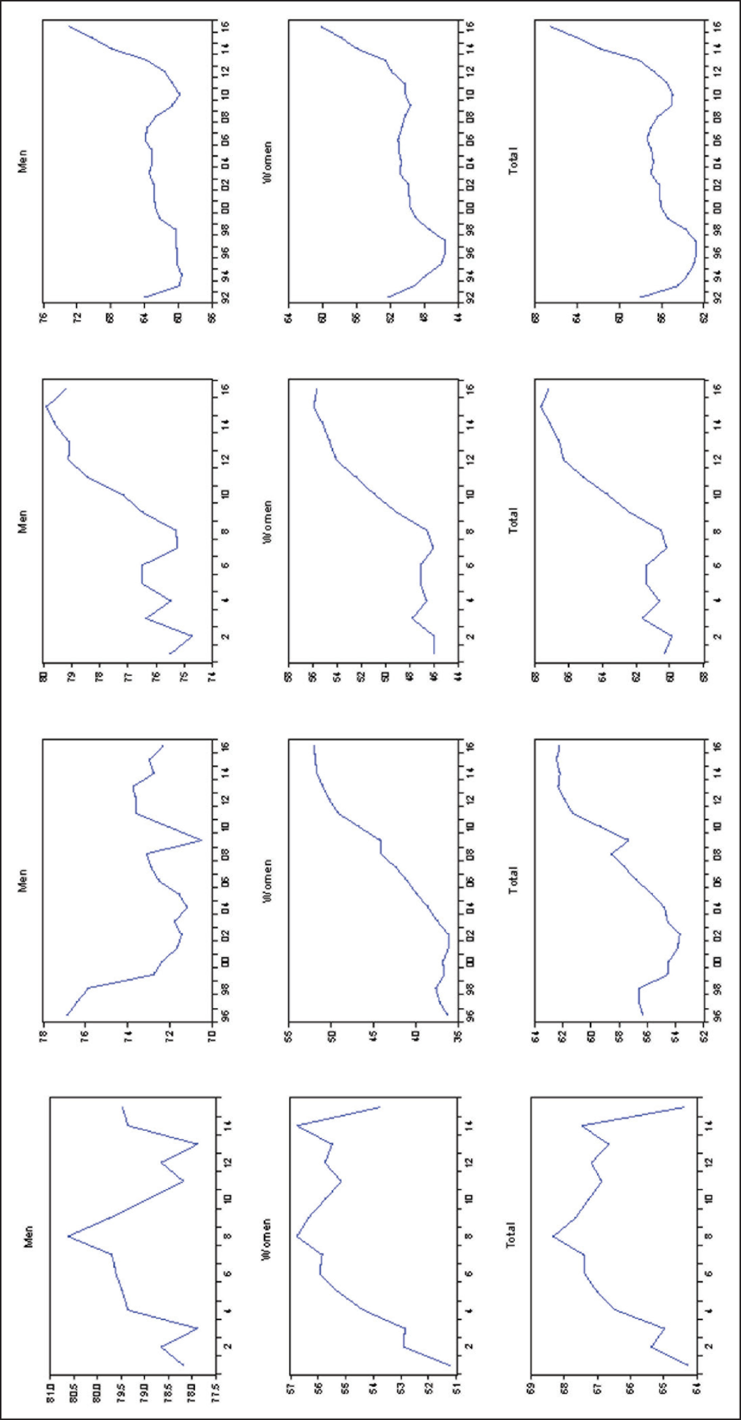
We now go over the hours worked data from various perspectives across time. Figure 1 shows the behaviour of total hours worked in EMEs from 1970 to 2013. We observe that there is a significant heterogeneity in the behaviour of hours in these economies. It displays a clear upward trend in Colombia, Peru and Sri Lanka while a persistent decline can be seen in the case of Hungary, South Africa and Turkey. To understand why changes in LS might be driving aggregate hours, the changes in total hours at the extensive (employment rate) and intensive (average hours per worker) margins are also illustrated in this figure. We find that total hours worked are shaped by both margins but it is obvious that it is mostly shaped by the movements in the extensive margin for all these economies. This makes us explore more about what drives the changes in extensive margin. Therefore, the changes in the extensive margin for both males and females between 16 and 64 years and the total are presented in Figure 3. For this, the data on employment-to-population ratio (the population aged 15–64) are compiled from the OECD database for Brazil (2001–2014), Chile (1996–2016), Colombia (2001–2016), Hungary (1992–2016), Mexico (1991–2016), Korea (1980–2015) and Turkey (1989–2015). It can be seen that the movements in the extensive margin for females contribute more to the variations in aggregate hours as the employment rate has been changing more for women than for men in these economies. More specifically, the extensive margin for women has increased notably in emerging countries included in our analysis such as in Brazil, from 51 to 57 per cent between 2002 and 2014; in Chile, from 35 to 53 per cent between 1996 and 2015 and in Mexico, from 34 to 46 per cent between 1992 and 2015. In Figure 4, we are able to look only the changes of intensive margins by gender in Mexico since it was not possible to obtain data for the other emerging economies. The data have been collected from Instituto Nacional De Estadistica Y Geografia (INEGI) from 1990 to 2015. It shows that there is a significant increase in the female intensive margin in Mexico between 1990 and 2015, while the male intensive margin dropped substantially between 2000 and 2006.

Figure 3

Notes: The figure shows the fluctuations in extensive margin by gender for EMEs. The countries from left to right: Brazil (2001–2015), Chile (1996–2016), Colombia (2001–2016), Hungary (1992–2016), Mexico (1991–2016), Korea (1980–2016) and Turkey (1988–2016). All variables are logged.

Figure 4

Notes: The figure shows the fluctuations of intensive margin by gender in Mexico from 1990 to 2015. The data are logged.

Lastly, the facts about the variations in home and market production are observed for available EMEs. The data for total weekly paid and unpaid work time (the sample included those aged between 15 and 64) are obtained from Bridgman, Duernecker, and Herrendorf (2015) for Korea (1970–2014) and Mexico (1992–2014). It is, thus, possible to examine only the home and market production hours for a few emerging economies, but this still enables an understanding of the changes in hours worked. The data show that the average weekly hours of household work in Korea and Mexico decreased from 20.8 to 10.4 per cent and from 34.6 to 29.9 per cent, respectively. However, market production increased from 28 to 32 per cent in Korea and from 30 to 35 per cent in Mexico. In addition, there was a decrease in home production (from 53 to 46 per cent) for women but an increase in market production (from 15 to 20 per cent) in Mexico. All these changes might be attributed to LS shocks and may reflect permanent shifts in hours worked.

The Augmented Dickey–Fuller (ADF) tests of the null hypothesis of non-stationarity and the Kwiatkowski–Phillips–Schmidt–Shin (KPSS) tests for stationarity on hours worked are presented in Table 1. The test results show that one cannot reject the hypothesis of a unit root (except for Mexico) and one can reject the hypothesis of stationarity at a very high significance level (except Sri Lanka and Thailand) for many EMEs. In addition, the same battery of ADF and KPSS tests applied to our GDP series supports the existence of a unit root and stationarity, respectively (see Figure 5). Finally, we observe that the test results provide support for the first-difference specification. Thus, we specify our variables as first differences in the VAR model in Section 3. Given that the data sample is annual, two lags are used following the convention in the literature.⁶ However, for a robustness check, we also check IRFs estimated using lags selected by the Akaike Information Criterion (AIC), the Schwarz Information Criterion (SIC) and Final Prediction Error (FPE) to determine the appropriate number of lags for our VAR model and then allow the lag length for each country. We start with a maximum of three lags. These tests show that one lag needs to be considered for Chile, Peru and Thailand, while two are required for Brazil, Mexico and South Korea and three are needed for Hungary, Sri Lanka and Turkey. Note that we do not use the US data when we run the structural VAR model in the next section. In this study, our focus is on the fluctuations in EMEs as the long-run behaviour of hours worked is more pronounced in EMEs. Hence, we only use the US data to show how hours worked data in EMEs are different than that of the USA.

Table 1

Tests of Non-stationarity and Stationarity

Countries	H₁	10%/5%/1%	H₂	10%/5%/1%
Brazil	–1.32	–3.59/–2.93/–2.60	1.37	0.74/0.46/0.35
Chile	–0.81	–3.59/–2.93/–2.60	1.32	0.74/0.46/0.35
Colombia	–0.35	–3.59/–2.93/–2.60	1.39	0.74/0.46/0.35
Hungary	–2.98	–3.59/–2.93/–2.60	1.34	0.74/0.46/0.35
Mexico	–3.64	–3.59/–2.93/–2.60	1.66	0.74/0.46/0.35
Peru	0.73	–3.59/–2.93/–2.60	2.08	0.74/0.46/0.35
South Korea	–0.79	–3.59/–2.93/–2.60	1.37	0.74/0.46/0.35
Sri Lanka	–1.95	–3.59/–2.93/–2.60	0.32	0.74/0.46/0.35
Thailand	–1.88	–3.59/–2.93/–2.60	0.19	0.74/0.46/0.35
Turkey	–2.76	–3.59/–2.93/–2.60	2.05	0.74/0.46/0.35

Notes: The table presents the results for the ADF unit root test H₁ and KPSS tests of stationarity H₂. t-statistics for the null hypothesis of a unit root and stationarity in the log-level of hours worked based on an ADF test and KPSS test with one lag and intercept. We choose the 1%, 5% and 10% levels as critical values. Sample period is 1970–2013.

Figure 5

Notes: The figure shows fluctuations of real GDP in EMEs. The data on GDP are total GDP, in millions of 1990 US dollars from 1970 to 2013 and are logged.

3. Methodology

In this section, the focus is on the SVAR procedure. The first step for the analysis of an SVAR is the estimation of a reduced form VAR:

D (L) X_{t} = ε_{t} E (ε_{t} ε_{t}^{'}) = Ω,

(1)

where D(L) = D₀ + D₁L + D₂L² + … + D₂L^p and L is the lag operator with LⁱX_t = X_t_-1. As Equation (1) is a reduced form, D₀ is equal to the identity matrix I. X_t is a vector of containing log hours worked (h_t) and real GDP(y_t). These variables into the VAR such that Dlog(h_t) is the first difference in the log of hours and Dlog(y_t) is the first difference of the log of real GDP. We invoke that these variables are driven by two shocks, LS shocks, $ε_{t}^{L S}$ , and technology shocks, $ε_{t}^{T S}$ , respectively. The covariance matrix of reduced form residuals ε_t is non-diagonal, and hence it is clear that the shocks in ε_t cannot be the structural innovations which are assumed to be uncorrelated with each other. When the VAR is invertible in Equation (1), the variables can be expressed as a moving average (MA) representation of the innovations ε_t:

X_{t} = C (L) ε_{t},

(2)

where C(L) = D(L)^-1. Now suppose that the VAR representation of the structural form can be written as:

B (L) X_{t} = u_{t} E (u_{t} u_{t}^{'}) = I, ​

(3)

where u_t are orthogonal structural disturbances which have been normalised so as to have unit variance, cov(u_t)=I. If the matrix polynomial D(L) is invertible, so is the matrix polynomial B(L) and then the MA representation with the structural shocks takes the following form:

X_{t} = A ​ (L) u_{t} .

(4)

Note that A(L) = B(L)^-1. The structural MA representation in Equation (4) is also called the final form of an economic model because the endogenous variables X_t are expressed as distributed lags of the exogenous variables, given by the elements of u_t. However, we cannot directly observe the structural shocks. We can observe the exogenous structural shocks u_t by first estimating the reduced form VAR (1) and then transforming the reduced form residuals. From Equations (2) and (4), we have:

A (L) u_{t} = C (L) ε_{t} .

(5)

As C₀ = 1 and Equation (5) must hold for all t, we have:

A_{0} u_{t} = ε_{t} .

(6)

It follows that:

A_{0} A_{0}^{'} = Ω,

(7)

It is obvious from Equation (7) that the matrix A₀ has to be of full rank. Combining Equations (5) and (6), we obtain:

A (L) u_{t} = C (L) A_{0} u_{t}, ​

(8)

which implies:

A_{i} = C_{i} A_{0} . ​

(9)

Note that knowledge of A₀ is sufficient for the full identification of the structural system. Identification requires choosing the n² elements of A₀. With a two-variable system, the A₀ matrix consists of four elements which necessitates four restrictions for identification. Structural shocks are supposed to be mutually uncorrelated, and therefore the variance–covariance matrix of the structural shocks need to be diagonal which yields n(n + 1)/2 restrictions on the elements of A₀, thereby imposing three restrictions on the elements of A₀. Additional n(n + 1)/2 restrictions are needed to fully identify A₀. From the theory model, we can impose the necessary restrictions following Blanchard and Quah (1989) who used long-run restrictions in order to identify structural VARs:

[\begin{matrix} Δ \log (h_{t}) \\ Δ \log (y_{t}) \end{matrix}] = [\begin{matrix} A_{11} (L) A_{12} (L) \\ A_{21} (L) A_{22} (L) \end{matrix}] [\begin{matrix} u_{t}^{L S} \\ u_{t}^{T S} \end{matrix}]

The long-run restriction makes A₁₂(1) = 0. In other words, the matrix of long-run multipliers A(1) is assumed to be lower triangular. We observe that one of the primary components of the business cycle might be LS shocks that can produce long-run changes in hours worked as we observe discernibly the variations in LS patterns in EMEs. Therefore, the identifying assumption imposed in the DSVAR is that LS shocks $u_{t}^{L S}$ are the only ones that can have an accumulated long-run effect on hours. Moreover, both LS and technology shocks have permanent effects on real GDP.⁷

4. A DSGE Model as Data-Generating Processes

In this section, our aim is to present an economic theory to test the claim made for the DSVAR procedure with long-run restrictions. Specifically, we present the models that are used to generate the simulated data for 1000 series for hours worked and GDP and then drop the first 956 for each variable in order to eliminate the effect of initial conditions. Later, we apply the DSVAR procedure to these data to see whether the BQ (Blanchard and Quah) procedure reveals the actual IRFs for emerging countries.⁸ As a benchmark, we build a DSGE model with non-stationary hours, due to a permanent preference shock (B_t), along the lines as given by Chang et al. (2006). The model is real and perfectly competitive. Households consume, accumulate physical capital and supply labour and capital to firms. In addition, there is a technology shock (A_t) which evolves according to a random walk as in a LS shock (B_t). For robustness, we also present a DSGE model with a productivity shock as a rate of growth shock as in Aguiar and Gopinath (2007). We are interested in their shock because they found that the business cycles in emerging countries are mainly driven by shocks to trend growth rather than transitory fluctuations around a stable trend. Finally, we build a DSGE model with both a productivity shock and a LS shock as a rate of growth shock. Note that these models satisfy completely the identifying assumption of the DSVAR specification as previously estimated in Section 3, this being only LS shocks that have a long-run effect on hours.

4.1 The Household Problem

The representative household maximises the expected discounted lifetime utility function from consumption C_t and hours worked H_t:

E_{0} [\sum_{t = 0}^{\infty} ​ β^{t} (\ln C_{t} - {(H_{t} / B_{t})}^{1 + 1 / ψ} 1 + 1 / ψ)] . ​

(10)

where E(.) denotes the expectation operator, conditional on information available at time t and b is the discount factor between 0 and 1. The Frisch LS elasticity is ψ. The log utility in consumption C_t implies a constant long-run LS in response to a permanent change in technology. H_t represents the hours worked, which are subject to a LS shock, denoted by B_t. If there is an increase in B_t, it leads to a rise in aggregate hours worked. A household is assumed to own capital, K_t, which accumulates according to the following law of motion:

K_{t + 1} = (1 - δ) K_{t} + I_{t}, ​

(11)

where I_t denotes investment and δ is the depreciation rate of capital. The households are subject to the following inter-temporal budget constraints:

C_{t} + I_{t} = W_{t} H_{t} + R_{t} K_{t}, ​

(12)

where W_t denotes a household’s real wage rate and R_t represents the rental rate of capital. Consumers choose to maximise utility, subject to capital accumulation and their budget constraint:

C_{t} + K_{t + 1} = W_{t} H_{t} + R_{t} K_{t} + (1 - δ) K_{t} .

(13)

4.2 The Firms Problem

The representative firm rents capital, hires labour and produces final goods according to the following Cobb–Douglas technology:

Y_{t} = K_{t}^{1 - α} {(H_{t} A_{t})}^{α},

(14)

where Y_t is output and α is the share of labour. The stochastic process A_t represents the exogenous labour augmenting technical progress. Profit maximisation of the firm and factor market equilibrium conditions determine the wage rate W_t and rental rate R_t:

R_{t} = (1 - α) {(\frac{K_{t}}{H_{t}})}^{- α} A_{t}^{α}, ​

W_{t} = α {(\frac{K_{t}}{H_{t}})}^{1 - α} A_{t}^{α} . ​

(15)

We assume that the log production (permanent) technology A_t and LS shock B_t evolve according to a random walk:

\ln A_{t} = \ln A_{t - 1} + ε_{a},_{t},

(16)

\ln B_{t} = \ln B_{t - 1} + ε_{b},_{t} .

(17)

ε_a,t and ε_b,t represent an independent and identical distribution drawn from a normal distribution, with a zero mean and standard deviation σ_a and σ_b, respectively. We use A₀ and B₀ to denote the initial level of A_t and B_t, respectively. Note that these shocks are orthogonal by construction. In this model, the B_t induces a stochastic trend into hours, output, consumption and capital. In addition, A_t has a long-run impact on output, consumption and capital but not on hours. That is, B_t is the only source of a stochastic trend in hours, while both shocks are the source of a stochastic trend in GDP. To obtain a stationary equilibrium, the variables have to be de-trended according to:

{\hat{H}}_{t} \equiv \frac{H_{t}}{B_{t}}, {\hat{Y}}_{t} \equiv \frac{Y_{t}}{A_{t} B_{t}}, {\hat{C}}_{t} \equiv \frac{C_{t}}{A_{t} B_{t}}, {\hat{K}}_{t} \equiv \frac{K_{t}}{A_{t} B_{t}} . ​

With these transformations, we have the following equilibrium dynamics of the endogenous variables in the neighbourhood of the steady state⁹:

Cobb–Douglas production function:

{\hat{Y}}_{t} = {\hat{K}}_{t - 1}^{1 - α} H_{t}^{α} {(\frac{A_{t} B_{t}}{A_{t - 1} B_{t - 1}})}^{α - 1} . ​

(18)

Labour demand:

{\hat{W}}_{t} = α {\hat{Y}}_{t} / H_{t} B_{t} .

Demand for capital:

R_{t} = (1 - α) {\hat{Y}}_{t} / {\hat{K}}_{t - 1} (\frac{A_{t} B_{t}}{A_{t - 1} B_{t - 1}}) . ​

LS:

{\hat{H}}_{t}^{1 / ψ} = {\hat{C}}_{t}^{- 1} {\hat{W}}_{t} .

Euler for capital:

{\hat{C}}_{t}^{- 1} = β {({\hat{C}}_{t + 1})}^{- 1} (\frac{A_{t} B_{t}}{A_{t + 1} B_{t + 1}}) (1 + R_{t + 1} - δ) . ​

Law of motion for capital:

{\hat{K}}_{t} = (1 - δ) {\hat{K}}_{t - 1} {(\frac{A_{t} B_{t}}{A_{t - 1} B_{t - 1}})}^{- 1} + {\hat{I}}_{t} . ​

Aggregate resource constraints:

{\hat{C}}_{t} + {\hat{K}}_{t} = {\hat{Y}}_{t} + (1 - δ) {\hat{K}}_{t - 1} {(\frac{A_{t} B_{t}}{A_{t - 1} B_{t - 1}})}^{- 1}, ​

{\hat{Y}}_{t} = {\hat{C}}_{t} + {\hat{I}}_{t} . ​

4.3 Calibration

We parametrise the parameter values that are familiar from the business cycle literature due to lack of quality data for annual frequency in emerging countries. Therefore, we have relied on highly conventional parameters widely used in the DSGE models of annual frequency for the USA. These values are fit for emerging countries. Table 2 reports all parameters of the model.

The labour share α is calibrated to match the capital share data. We hence set α in production to 0.68, which is a standard value for the long-run labour share income so that the value of capital share is set to 0.33 to match the average fraction of total income going to capital in emerging countries. The discount factor β is calibrated to match the steady-state capital–output ratio in the capital Euler equation to that in data. The value of β used in the literature ranges from 0.92 to 0.99 for annual frequency for emerging countries. We set β to 0.95 in order to imply a steady-state real interest rate at about 5 per cent per year which is a value compatible with the observed interest rate faced by emerging countries.¹⁰ We set the inverse of the Frisch elasticity of the LS ψ of the utility function to 0.33 so that it matches the steady-state labour input level in the labour first-order condition to that in the data which are commonly used in the RBC (Real business-cycle) literature. The value of the depreciation rate δ ranges from 0.03 to 0.12 per year for emerging countries in the literature. We have used a 7 per cent annual depreciation rate to match the capital law of motion as it falls in the middle of that range.¹¹ The standard deviation of the technology shocks, σ_a, and the LS shocks, σ_b, are calibrated to 1.2 and 0.6 per cent, respectively, as given in Chang et al. (2006) who estimate a DSGE model with non-stationary hours using Bayesian techniques.¹²

Table 2
Parameters Values in the Models

Parameters Definition Value

β The discount factor 0.95

ψ The inverse of the Frisch elasticity of LS 0.33

α The labour share of output 0.68

δ The depreciation rate of capital 0.07

μ The long-run average growth rate of shocks log(1.0066)

ρ The persistence of growth shocks 0.01

σ_a The standard deviation of technology shocks 0.012

σ_b The standard deviation of LS shocks 0.006

Parameters	Definition	Value
β	The discount factor	0.95
ψ	The inverse of the Frisch elasticity of LS	0.33
α	The labour share of output	0.68
δ	The depreciation rate of capital	0.07
μ	The long-run average growth rate of shocks	log(1.0066)
ρ	The persistence of growth shocks	0.01
σ_a	The standard deviation of technology shocks	0.012
σ_b	The standard deviation of LS shocks	0.006

Notes: The table shows the parameter values in the DSGE models. Note that we assume that the persistent of the permanent LS shocks is ρ_b = ρ_a= ρ and the long-run average growth rate of LS shocks μ_a = μ_a = μ.

5. Results

To evaluate the DSGE model, we resort to the Indirect Inference approach. Accordingly, we estimate a DSVAR model on simulated data from the DSGE model and compute the impulse responses of hours and GDP to technology and LS shocks using long-run restrictions. The accumulated IRFs are then compared with those obtained from actual data in EMEs using annual data for the period 1970–2013, as well as their 95 per cent confidence intervals. Recall that the only identifying assumption imposed in the DSVAR is that LS shocks have a permanent effect on hours worked yet technology shocks do not have long-run effects on hours. It also supports the long-run restrictions imposed in the DSGE model. These LS shocks can be an important source of fluctuations as we observe persistent fluctuations in LS following changes in labour market participation or changes in the demographic structure in EMEs. In addition, we consider larger VAR specifications by adding consumption-to-output ratio (See Figure 6) for the robustness of our first results as well as different shock process for the DSGE models. The standard error bands are computed using a bootstrap procedure with 1000 replications.

We first present the results based on a simple bivariate VAR model with two lags. The accumulated IRFs of hours and GDP after a LS shock and a technology shock are reported in Figure 7 for each county. Several salient features emerge from our DSVAR. (1) It shows that both a technology shock and a LS shock lead to an immediate and permanent rise in real GDP for all the EMEs, though not statistically significant in the long run. It rises during 2–3 periods, and the response remains positive for each horizon. Only in Sri Lanka, following a LS shock, real GDP increases on impact but decreases after one period and then the response remains negative. (2) In response to the technology shocks, hours worked decline temporarily in Brazil, Hungary and Turkey. It increases in Chile, Mexico, Peru, Sri Lanka and Thailand but eventually the effect of the technology shocks on hours disappears over time (by assumption). For Colombia and South Africa, technology shocks have a negative impact initially but then return a positive effect on hours worked insignificantly. (3) The impact of the (identified) permanent LS shocks on hours worked are positive. It increases for about 1 year and eventually reaches a new steady state higher than its pre-shock level.

Figure 6

Notes: The figure displays the behaviour of the consumption-to-output ratio in EMEs from 1970 and 2013. Household consumption expenditure data are used at current prices in US dollars, including non-profit institutions serving households and the data on GDP are total GDP, in millions of current US dollars. The data are logged.

Figure 7

Note: The figure shows the accumulated impulse responses of hours and real GDP to technology and LS shocks (blue solid lines) and the 5 and 95 per cent confidence bands (black dashed lines) using the two-lag DSVAR procedure with EMEs data set.

Our empirical framework includes two driving forces which are LS and technology shocks. However, Blanchard and Quah (1989) pointed out that ignoring some relevant shocks may lead to a significant distortion in the estimated impulse responses. To ensure that the VAR procedure works well, we add an extra control variable, i.e. the consumption-to-output ratio (C/Y) to the VAR to see whether our model is robust. We include it because it improves the identification of the technology shocks and displays less controversy about its stationarity in the literature (Gospodinov, 2010). Moreover, Cochrane (1994) contended that the C/Y ratio is special because it is stable over long time periods (consumption and output are co-integrated), while consumption is nearly a random walk. The A(L) matrix of this system is a block 3 × 3 matrix in the lag operator and we specify the three-variable model as follows:

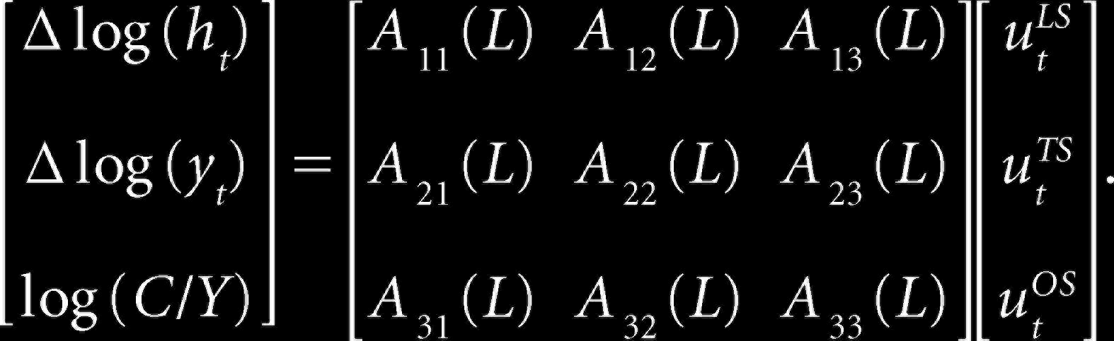
[\begin{matrix} Δ \log (h_{t}) \\ Δ \log (y_{t}) \\ \log (C / Y) \end{matrix}] = [\begin{matrix} \begin{matrix} A_{11} (L) & A_{12} (L) & A_{13} (L) \end{matrix} \\ \begin{matrix} A_{21} (L) & A_{22} (L) & A_{23} (L) \end{matrix} \\ \begin{matrix} A_{31} (L) & A_{32} (L) & A_{33} (L) \end{matrix} \end{matrix}] [\begin{matrix} u_{t}^{L S} \\ u_{t}^{T S} \\ u_{t}^{O S} \end{matrix}] .

The estimates generated by that higher dimensional model regarding the effects of shocks are very similar to the ones reported earlier. If the hours worked is the first variable in the system, we identify the LS shocks by imposing the restriction that $A^{1 j} (1) = 0 $ for j = 2, 3. This framework shows that two shocks, consisting of technology shocks and other shocks (OS), do not have a permanent effect on hours. Furthermore, LS and technology shocks and not OS have a permanent effect on GDP, that is A₂₃ = 0. Lastly, none of these shocks will have a permanent effect on C/Y because we assume that it is stationary in level in our VAR analysis. The pattern of responses of hours and GDP to both shocks is very similar to that obtained in the bivariate model for all countries. Although adding the consumption-to-output ratio into the VAR does not modify the previous results in most cases, we definitely obtain more pronounced results compared with the two-variable VAR model. For robustness, we also check IRFs estimated using lags selected by the lag-length tests suggested. We observe slightly more significant results if we estimate our DSVAR model for Chile, Peru and Thailand (with one lag) and Hungary, Sri Lanka and Turkey (with three lags).

We then generate 1000 data samples for hours worked and real GDP from the DSGE model. Every data sample consists of 44 annual observations and corresponds to the typical sample size of empirical studies. That is, in order to reduce the effect of initial conditions, the simulated samples include 956 initial points which are subsequently discarded in the estimation. For every data sample, we estimate VAR models with two lags. Before applying VAR procedure, we consider the unit root tests by conducting an ADF and a KPSS tests on simulated series. We find that the test does not reject a unit root but can reject the hypothesis of stationarity in hours worked, respectively.

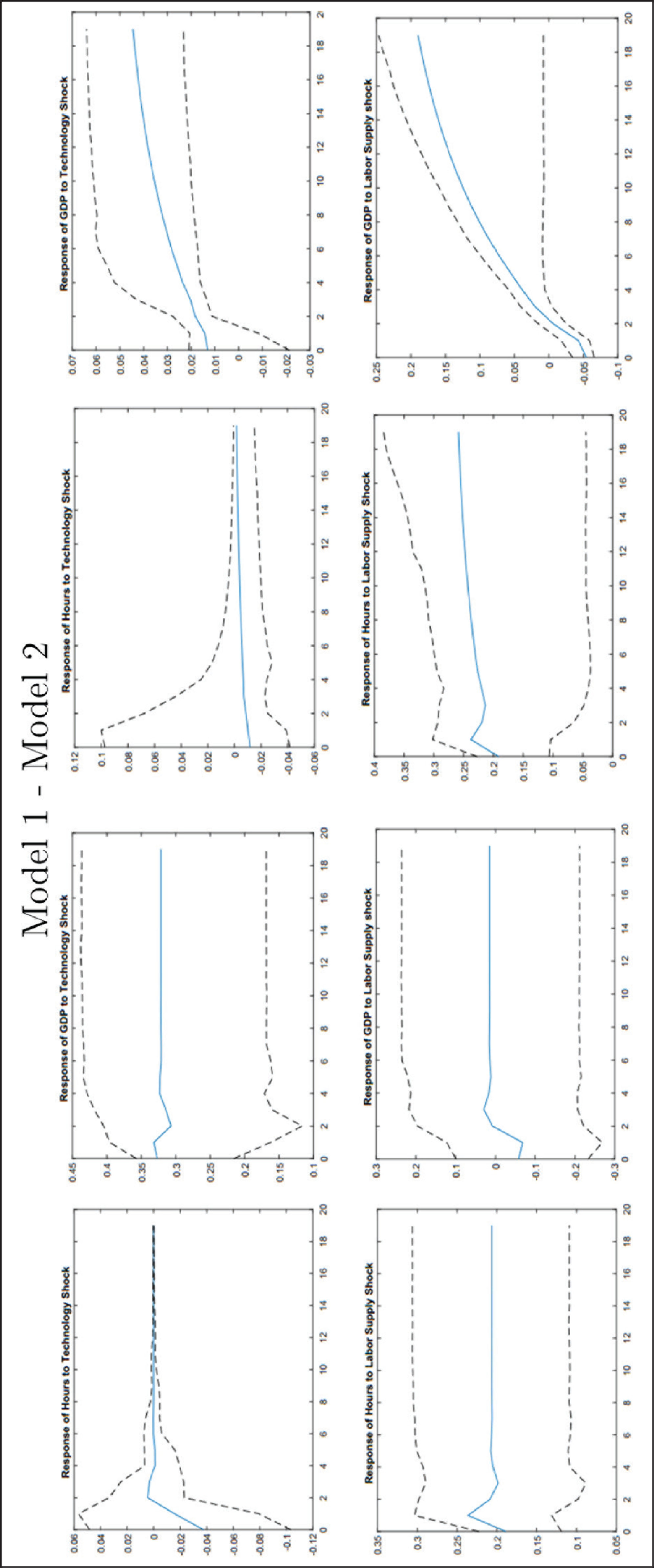
In our benchmark model, we assume that both shocks evolve according to the random walk (Model 1). Figure 8 shows the IRs of hours and GDP to LS and technology shocks from the estimated DSVAR on the artificial data. We observe that hours rise permanently after a positive LS shock but it does so only rises for one period. The dynamic response of technology shocks on hours is negative and these shocks do not have any long-run effect on hours. Also, GDP increases permanently after a positive technology shock. Following LS shocks, real GDP decreases in the beginning of the period but then increases permanently. We observe that the DSVAR is not able to capture the significant impulse responses of this model. For robustness, we first build a DSGE model by following the same procedure as earlier with the shocks to trend growth of productivity (Model 2), and hence the permanent labour-augmenting productivity shock, A_t, is non-stationary and represents the cumulative product of growth shocks. It is given by:

A_{t} = a_{t} A_{t - 1} = \prod_{s = 0}^{t} ​ a_{s}, ​

\ln (a_{t}) = (1 - ρ_{a}) \log (μ_{a}) + ρ_{a} I n (a_{t - 1}) + ε_{t}^{a} . ​

We then build a DSGE model with both a productivity shock and a LS shock as a rate of growth shock again following the same procedure described earlier (Model 3). That is, the permanent LS shocks, B_t, is non-stationary and represents the cumulative product of growth shocks b_t:

B_{t} = b_{t} B_{t - 1} = \prod_{s = 0}^{t} ​ b_{s}, ​

\ln (b_{t}) = (1 - ρ_{b}) \log (μ_{b}) + ρ_{b} I n (b_{t - 1}) + ε_{t}^{b} . ​

Figure 8

Notes: The figure shows the accumulated impulse responses of hours and real GDP to technology and LS shocks (blue solid lines) and the 5th and 95th per cent confidence bands (black dashed lines) using the two-lag DSVAR procedure with the simulated data set. In Model 1, we assume that the log production (permanent) technology A_t and LS shocks B_t evolve according to a random walk. In Model 2, we assume that there are the shocks to trend growth of productivity. In Model 3, we assume both productivity and LS shocks as a rate of growth shock.

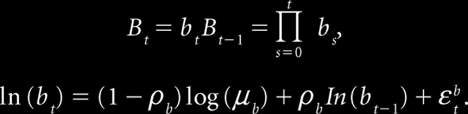
In these models, the parameters a_t and b_t represent the rate of growth of the permanent technology shock and LS shock, respectively. |ρ_a| < 1and |ρ_b| < 1 are the persistence parameters of the process a_t and b_t, respectively. $ε_{t}^{a} $ and $ε_{t}^{b} $ represent iid drawn from a normal distribution with a zero mean and standard deviation σ_a and σ_b, respectively. μ_a and μ_b are the long-run average growth rate of both shocks. The persistence of the permanent technology shocks ρ_a and the long-run average growth rate of technology shocks μ_a are set to 0.01 and to log (1.0066), respectively as given by Aguiar and Gopinath (2007). Note that we assume that the persistence of the permanent LS shocks ρ_b and the long-run average growth rate of LS shocks μ_b are equal to the ones in that of permanent technology shocks. We make this assumption based on the observation we made in the literature but we could not find any value for them in the literature. Chang et al. (2006) estimated the persistence of the temporary LS shocks in the stationary model and found that it is equal to 0.95, which is also equal to the value for the persistence of the temporary productivity technology shocks as given by Aguiar and Gopinath (2007). Hence, we assume that ρ_a and μ_a can be equal to ρ_b and μ_b, respectively (see Table 2).

We observe that the pattern of the IRFs does not change much but it seems that the VAR model is better at capturing the dynamic response of LS and technology shocks on hours worked and real GDP in Models 2 and 3 compared with the results from the benchmark model. Moreover, the response of GDP to technology shocks and LS shocks is different only in Model 3 compared with the benchmark and second model. The effect of technology shocks on GDP is initially negative and then returns to positive in the long run, and LS shocks have a positive permanent impact on real GDP in this model.

These results allow us to compare empirical impulse responses based on the actual data to impulse responses from DSVARs run on the simulated data from the models. There are four main conclusions that can be drawn. First, it seems that the response of hours to technology shocks are consistent in the data and in the model for Brazil, Hungary and Turkey where following a technology shock, hours decrease. Secondly, our models can produce the impulse response of hours after LS shocks for all emerging economies where these shocks increase hours worked permanently in the long run. Moreover, Models 2 and 3 are better to capture the response of hours worked to LS shocks compared with the benchmark model. Thirdly, in our benchmark and second model we find that the response of GDP to technology shocks is positive in the long run which imitates the pattern of IRFs from the DSVAR for all EMEs. In Model 3, real GDP also increases permanently but initial effect of a positive technology shocks is negative. Lastly, in the model with both a productivity shock and a LS shock as a rate of growth shock, we find that real GDP rises permanently after a LS shock. We observe that this model can produce similar patterns to those in EMEs (except in Sri Lanka).

The overall results show that our models are able to indirectly mimic IRFs obtained from a DSVAR on the actual data although our DSVAR specification poorly identifies the impulse responses of hours worked and real GDP to both shocks. We can conclude that a DSGE model with permanent LS shocks that can generate a unit root in hours worked has a better time-series fit for EMEs and matches with the empirical findings. Therefore, a model with LS shocks is required to properly evaluate the DSVAR in EMEs as the data support this view. In addition, these shocks can be the driving force behind business cycle fluctuations in EMEs as they can explain the movements in hours worked.

6. Conclusion

In this paper, we test a DSGE model using indirect inference on impulse responses of hours worked and real GDP after technology and non-technology shocks in EMEs. We observe that the behaviour of hours worked is non-stationary between 1970 and 2013 in these economies but many dynamic macroeconomic models assume that hours worked are stationary. Based on these observations, we provide empirical evidence on the impact of technology and non-technology shocks on hours and GDP using DSVAR model. As a data-generating process, we then illustrate that DSGE models can be easily modified to incorporate non-stationary LS shocks which generate permanent shifts in hours worked. This model satisfies completely the identifying assumption of the DSVAR specification, i.e. only LS shocks can have a long-run impact on hours worked. We then compare the responses of hours and GDP in DSVAR model obtained using data generated by the estimated theoretical model with those obtained using actual data. Our main findings are that (1) hours increase permanently after a positive LS shock in these economies and (2) LS shocks can be the main driving force behind business cycle fluctuations in EMEs which are able to replicate the impulse responses of the DSVAR if the model and actual data are treated symmetrically. In this study, we emphasise that the changes in the structure of labour markets in these economies can account for permanent shifts in hours worked especially the changes in female labour force participation. Therefore, more work must be undertaken to understand economic factors behind the fluctuations in hours worked without violating the balanced growth hypothesis, so that a model with household’s labour force participation may be worthwhile exercised focusing on more sophisticated DSGE models with real and nominal frictions for future research.

Footnotes

Acknowledgements

I am grateful to Miguel Leon Ledesma, Peter J. N. Sinclair, Mathan Satchi and audiences at the EBES conference as well as seminar participations at Kent and anonymous referees at this journal for valuable comments and suggestions.

Declaration of Conflicting Interests

The author declared no potential conflicts of interest with respect to the research, authorship and/or publication of this article.

Funding

The author received no financial support for the research, authorship and/or publication of this article.

The First-Order Conditions of the Model and Steady States—Benchmark Model

The first-order conditions of consumption, hours and capital, respectively, are given by: (19)

λ_{t} = C_{t}^{- 1},

H_{t}^{1 / ψ} B_{t}^{- (1 + 1 / ψ)} = C_{t}^{- 1} W_{t},

λ_{t} = β λ_{t + 1} (1 + R_{t + 1} - δ) .

Since all the variables in Equation (18) are stationary (see Section 4), we can compute a steady-state, dropping time subscripts. The solution for the steady state of the model is as follows. The rental rate of capital: (20)

R = 1 β - (1 - δ),

The output-to-capital ratio is derived from the marginal product of capital and $R$ which are equal to each other:

Y K = R (1 - α),

The investment to output ratio is derived from capital equation:

I Y = 1 Y / K δ,

The consumption-to-output ratio is obtained from the budget constraint:

C Y = 1 - I Y,

Hours can be derived from the marginal rate of substitution between leisure and consumption equation:

H = α {(1 C / Y)}^{ψ / (1 + ψ)},

Capital is derived from the rental rate of capital equation: (25)

K = {(H^{α} Y / K)}^{1 / α},

Output is derived from the Cobb–Douglas production equation:

Y = K^{1 - α} H^{α},

Consumption is from the consumption-to-output ratio and output:

C = C Y Y,

Investment is obtained from the investment-to-output ratio and output:

I = I Y Y,

Wages:

W = α Y H .

Notes

References

Aguiar

, & Gopinath

(2007). Emerging market business cycles: The cycle is the trend. Journal of Political Economy, 115, 69–102.

Basu

, Fernald

, & Kimball

(2004, June). Are technology improvements contractionary? Working Paper 10592, National Bureau of Economic Research.

Blanchard

O. J.

, & Quah

(1989, September). The dynamic effects of aggregate demand and supply disturbances. American Economic Review, 79(4), 655–673.

Boppart

, & Krusell

(2016, May). Labor supply in the past, present, and future: A balanced-growth perspective. Working Paper 22215, National Bureau of Economic Research.

Bridgman

, Duernecker

, & Herrendorf

(2015, October). Structural transformation, marketization, and household production around the world. BEA Working Papers 0128, Bureau of Economic Analysis.

Canova

, & Sala

(2009). Back to square one: Identification issues in DSGE models. Journal of Monetary Economics, 56(4), 431–449.

Cantore

, Ferroni

, & Leon-Ledesma

M. A.

(2017). The dynamics of hours worked and technology. Journal of Economic Dynamics and Control, 82, 67–82.

Cantore

, Leon-Ledesma

, McAdam

, & Willman

(2014). Shocking stuff: Technology, hours, and factor substitution. Journal of the European Economic Association, 12(1), 108–128.

Chang

, Doh

, & Schorfheide

(2006). Non-stationary hours in a DSGE model. Technical report.

10.

Chang

, & Schorfheide

(2002, May). Labor-supply shifts and economic fluctuations. Macroeconomics 0204005, EconWPA.

11.

Chaudourne

, Feve

, & Guay

(2014). Understanding the effect of technology shocks in {SVARs} with long-run restrictions. Journal of Economic Dynamics and Control, 41, 154–172.

12.

Christiano

L. J.

, Eichenbaum

, & Vigfusson

(2003, July). What happens after a technology shock? NBER Working Papers 9819, National Bureau of Economic Research.

13.

Cochrane

J. H.

(1994). Permanent and transitory components of GNP and stock prices. The Quarterly Journal of Economics, 109(1), 241–265.

14.

Cogley

, & Nason

J. M.

(1995, June). Output dynamics in real-business-cycle models. American Economic Review, 85(3), 492–511.

15.

Dupaigne

, Fève

, & Matheron

(2007). Avoiding pitfalls in using structural vars to estimate economic models. Review of Economic Dynamics, 10(2), 238–255.

16.

Dupaigne

, Feve

, & Matheron

(2005). Technology shock and employment: Do we really need DSGE models with a fall in hours? Technical report.

17.

Francis

, & Ramey

V. A.

(2005a). Is the technology-driven real business cycle hypothesis dead? Shocks and aggregate fluctuations revisited. Journal of Monetary Economics.

18.

Francis

, & Ramey

V. A.

(2005b, October). Measures of per capita hours and their implications for the technology-hours debate. Working Paper 11694, National Bureau of Economic Research.

19.

Francis

, & Ramey

V. A.

(2004, July). The source of historical economic fluctuations: An analysis using long-run restrictions. NBER Working Papers 10631, National Bureau of Economic Research.

20.

Gali

(2004). On the role of technology shocks as a source of business cycles: Some new evidence. Journal of the European Economic Association, 2(2–3), 372–380.

21.

Gali

(1999, March). Technology, employment, and the business cycle: Do technology shocks explain aggregate fluctuations? American Economic Review, 89(1), 249–271.

22.

Gali

(2005, February). Trends in hours, balanced growth, and the role of technology in the business cycle. Working Paper 11130, National Bureau of Economic Research.

23.

Gali

, & Rabanal

(2005, April). Technology shocks and aggregate fluctuations: How well does the real business cycle model fit postwar U.S. data? (pp. 225–318). MIT Press.

24.

Garcia-Cicco

, Pancrazi

, & Uribe

(2010, December). Real business cycles in emerging countries? American Economic Review, 100(5), 2510–2531.

25.

Gospodinov

(2010). Inference in nearly nonstationary SVAR models with long-run identifying restrictions. Journal of Business & Economic Statistics, 28(1), 1–12.

26.

Hall

R. E.

(1997, January). Macroeconomic fluctuations and the allocation of time. Journal of Labor Economics, 15(1), 223–250.

27.

King

R. G.

, Plosser

C. I.

, & Rebelo

S. T.

(1998). Production, growth and business cycles: I. The basic neoclassical model. Journal of Monetary Economics, 21(2–3), 195–232.

28.

(2011, October). Cyclical wage movements in emerging markets compared to developed economies: The role of interest rates. Review of Economic Dynamics, 14(4), 686–704.

29.

McGrattan

E. R.

, & Rogerson

(2004, July). Changes in hours worked, 1950–2000. Quarterly Review, 28(1), 14–33.

30.

Minford

, Wickens

, & Xu

(2016). Comparing different data descriptors in indirect inference tests on DSGE models. Economics Letters, 145, 157–161.

31.

Shapiro

M. D.

, & Watson

M. W.

(1988, May). Sources of business cycle fluctuations. Working Paper 2589, National Bureau of Economic Research.

32.

Sims

C. A.

(1980, January). Macroeconomics and reality. Econometrica, 48(1), 1–48.