Is the Relationship Between Government Spending and Private Consumption in Egypt Symmetric?

Abstract

The aim of this study, using Egyptian data from 1970 to 2016, is to explore the relationship between government spending and private consumption spending and to understand whether the relationship between the two is symmetric. The study uses the autoregressive distributed lag (ARDL) approach to explore a cointegration relationship between the two variables, and the nonlinear autoregressive distributed lag (NARDL) approach to test the hypothesis of a symmetric relationship between the two variables. By applying the ARDL approach, the study concludes that the effect of government spending on consumption spending is not significant in the long term. By applying the NARDL approach, the study concludes that: the hypothesis of the presence of a symmetric relationship is not accepted, there is a crowding-out relationship from the positive shocks of government spending and the substitutability coefficient between the two types of spending is 0.8699.

JEL Classification: E12, E21, F62, H50

Keywords

Government Spending Private Consumption Egyptian Economy Crowding-out Relationship Symmetric Relationship

1. Introduction

Research on consumption behaviour is important in the context of identifying the prevailing economic-social behaviours in any country. Consumption spending represents the most important rate of total spending, exceeding, in developing countries’ economies, approximately 90 per cent of total national income but falling back to approximately 60 per cent in rich countries’ economies. The large economic theories, especially the classical and Keynesian schools, have different opinions concerning studying the relationship between governmental and private consumption spending. The applied studies also do not have the final word on the nature of this relationship.

While the new classical theory and the real business cycle (RBC) theory confirmed the inverse relationship (crowding out) between the two variables, Keynesian theory adopts the opinion that the relationship is a direct (integrating) one (Baxter & King, 1993). The hypothesis of a crowding-out relationship between the two types of spending is based on the point that governmental spending is covered or financed by taxes that are deducted from personal income. Accordingly, high government spending means that an increase in taxes is needed; thus, disposable income (personal income − taxes + governmental financial transfers) decreases. Particularly in developing countries, where the marginal propensity to consume is high, it is expected that tax increases will be at the expense of the provision of consumption spending from disposable income. In other words, government spending will crowd-out consumption spending. In another case, when the government turns to finance its spending through increasing note issues (deficit financing), inflation pressures resulting from that approach will negatively affect the consumption spending of individuals (Khan et al., 2015).

The other hypothesis (hypothesis of the integration relationship between the two types of spending) suggested by supporters of Keynesian theory is a supplement to the defence rendered by Keynes about the role of government in the positive effect on effective total demand and activating the economic cycle. In this case, the government increases the number of employees in its institutions, transfers of money to unemployed persons and spending on infrastructure, which results in derivative demand for the workforce and an increase in the salaries paid by the government directly or through contractors. All these procedures increase national income and improve the level of income of individuals so that they transfer their acquired incomes to consumption spending in light of an increase in the marginal propensity to consume for a wide section of individuals.

In general, the two models (the Keynesian model and the new classical model) support the idea that government spending has a double effect on the outcome. The efficiency of this effect is based upon the size of the multiplier, which in turn is affected by the marginal propensity to consume. The size of that multiplier is based on a mechanism of the response of private consumption spending to changes in government spending. At this point, the Keynesian model predicts that the effect of the government spending is direct, while the RBC model predicts that it has a negative effect.

Other economists, such as Bailey (1971) and Barro (1981), think that a direct effect of government spending on private consumption spending may happen. Government purchasing of goods and services will affect the total benefit of all consumers. In this case, the response of private consumption to government spending is affected by the substitutability or complementarity coefficient between the two variables.

This study tries to research the effect of changes in government spending on the consumption function behaviour in the long term and the short term. Specifically, the effect of government spending on consumption spending will be discussed; accordingly, the nature of this effect will be tested in terms of both the positive and negative changes resulting from that spending. This procedure is technically referred to as testing the symmetric relationship between the two variables.

The study hypothesizes that the relationship between the two variables is an integration relationship in which the increase in government spending leads to an increase in private consumption spending in the long term.

Based on data from the Egyptian economy, the study also hypothesizes that there is a direct relationship between government spending and private consumption spending and that this relationship is asymmetric. In other words, the positive change in government spending is not necessarily equal to the negative changes from its effect on consumption spending. The effect of the positive shock on government spending is different from the effect of the negative shock of that spending on private consumption spending.

This study is important, as it tests a hypothesis not tested previously in the world economic literature (to the best knowledge of the researcher and based on reviewing the scientific research engines on the internet), although the economic literature has few studies about the relationship between the two types of spending specifically in Egypt. Therefore, this study is a preliminary contribution to testing this hypothesis in the world economic literature.

This study is also important because it provides information about the behaviour of the consumption function and the effect of changes from governmental spending in Egypt. This information may form a basis that helps political and economic decision-makers to address the financial policy of the country, to predict consumer behaviour in the local market resulting from changes in this policy and to control the paths of this behaviour in accordance with Egyptian future development plans.

For this purpose, the study uses the nonlinear autoregressive distributed lag (NARDL) approach, in which the hypothesis of the symmetric relationship between consumption and government spending will be tested.

Guided by the scientific method adopted in this type of study, the study in addition to the introduction is divided into the theoretical framework and previous studies, study method, study data, estimation method adopted in exploring the hypothesis, applied framework, which in turn includes identifying the exploration of the statistical characteristics of the study data and the model estimation, and the discussion of the results in the last part of the study.

2. Theoretical Framework and Previous Studies

In many previous studies, the relationship between consumption spending and government spending did not evidence a specific trend. Many studies stated that the relationship is a reversal (crowd out), while other results confirmed that the relationship between the two is direct.

One of the oldest studies, which tested the relationship between public and private spending, is of Bailey (1971), who concluded that there is a crowd-out relationship between the two and did not accept the Keynesian hypothesis with respect to this relationship.

One study that concluded that there is a reversal relationship directing from government spending to private consumption spending was of Ho (2001). The study discusses the crowd-out and integration relationship between government spending and private consumption spending. The study concluded that its results enhance the empirical literature by using the standard panel data approach. In this regard, the study used the cointegration approach concerning this type of data. The results from 24 Organisation for Economic Co-operation and Development (OECD) country economies mentioned that there is a crowd-out relationship to a great degree between government spending and private consumption spending when using available real income and not permanent income. The study concludes that the Keynesian hypothesis is not accepted and considers it unconvincing.

Bouakez and Rebei (2007) also reached a similar conclusion using data from the United States for the period from 1952 Q1 to 2001 Q4. The two researchers developed a small economic cycle model to follow up on the effect of government spending on private consumption spending. Their conclusion was to not accept the Keynesian hypothesis that says that the relationship between the two types of spending is an integration relationship, but they confirmed that the relationship may be integrative in the case of using total governmental spending rather than specific spending items.

Using panel data from East Asia countries, Kwan (2006) also concluded that there is a crowd-out relationship between the two types of spending. The researcher used data for the period 1960–2002. Empirical analysis results state that the substitutability elasticity coefficient in China, Japan, Hong Kong and Korea was mild, whereas it was high in Malaysia and Thailand and zero in the Philippines.

On the other hand, many studies determined that the relationship between the two types of spending is direct. For example, Evans and Karras’s (1996) is considered one of the first studies to note that the relationship between the two variables (government spending and private consumption spending) is an integration relationship (and not a crowd-out relationship). The study tested its hypothesis by using annual data for 52 countries.

Coenen and Straub (2005) tried to reconsider the effect of government spending shocks on private consumption spending in the Euroregion. The study concluded that there is to some extent a small opportunity for gathering governmental shocks in consumption not only mainly because the estimative share of the families is relatively low but also because of the large negative effect of wealth resulting from the nature of the governmental spending shocks.

Hafedh and Nooman (2007) used data from the United States to test the relationship between governmental spending and private consumption spending. The study concluded that there is a strong relationship between the two variables. The study also states that the private consumption response to governmental spending shocks is positive by using the impulse response function generated by the VAR model.

Bernardini and Peersman (2018) tried to prove that the relationship between governmental spending as an explanative variable and private consumption spending as a dependent variable is an integration relationship in China. For this purpose, the researchers used the autoregressive distributed lag (ARDL) approach on data from the period 1985–2013. The study concluded that governmental spending directly affects private consumption spending.

Samadi and Sayedi (2012) concluded that there is a direct relationship from governmental spending to private consumption spending in Iran. The study used the mathematical frame submitted by D’Alessandro (2010), and the study tested its hypothesis by using the ARDL approach and data for the period 1959–2007.

Durkaya (2012) submitted evidence that supports the Keynesian approach. The study concluded that the relationship between governmental spending and private consumption spending is a direct relationship in the long term and the short term in Turkey during the period 1980–2010. The study used the cointegration approach and error correction and stated that the elasticity coefficient in this relationship is 0.52.

Ercolani and Pavoni (2012) built a unique database that connected the private consumption of families to the governmental consumption of the region in which the families lived in Italy. The study used the regional fluctuations of the governmental consumption and measured its effect on the individual consumption of different categories of governmental spending. The study reached two main conclusions:

Spending of the families increased as long as the consumption spending varied.

Public healthcare has a negative effect on variation in the living spending of the families.

The study done by Khan et al. (2015) supported the existence of a direct relationship between the two types of spending in the Chinese case based on annual data from 1985 to 2013. The study used the ARDL approach. It concluded that governmental spending is an important tool for enhancing the economy and encouraging total demand in China during a stagnation period.

The above review of a variety of previous studies clearly shows that the trend of the relationship between the two types of spending is not decided, thus justifying an exploration of this relationship, particularly given that studies about Arab countries are rare. I also am unaware of any previous studies using the NARDL approach for testing a hypothesis of the presence of a symmetric relationship between the two types of spending.

This study tries to fill this gap by testing the relationship between governmental spending and private consumption spending in the Arab countries and by using an approach different from the approaches used in the previous studies, that is, the NARDL approach.

3. Study Model, Estimation Method, Study Data

3.1 Study Model

Taking into consideration the theory, research hypothesis and previous studies, it is possible to form the study model as the following:

l C_{t} = α + β l G_{t} + μ_{t}

(1)

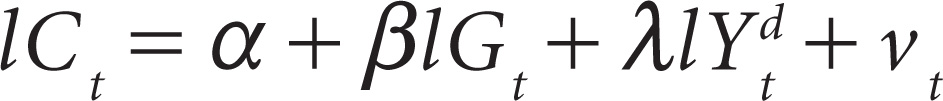
where LC_t is the natural logarithm of the share of the individual in private consumption spending at fixed 2010 prices in year (t), LG_t is the natural logarithm of the share of the individual of government spending at fixed 2010 prices in year (t), and µ_t is the error limit. Using the logarithm in the estimation is important for obtaining the elasticity of the relationship between consumption spending and government spending.

Commenting on the previous model, Graham (1993) mentioned that adding real disposable income will affect the strength of the effect of government spending on private consumption spending and that excluding real disposable income will weaken the strength of that relationship. Therefore, it is proper to test the previous relationship after adding the natural logarithm of the share of the individual of real disposable income Yd so that the second model to be estimated becomes the following:

l C_{t} = α + β l G_{t} + λ l Y_{t}^{d} + v_{t}

(2)

Some studies, such as Shaikh’s (2018), added other variables such as a wealth variable, real rate of interest or discount rate and unemployment rate. In this study, quasimoney was used as a proxy for the wealth of the national sector, while the unemployment rate was used as a proxy for uncertain income. Taking into consideration that data related to the rates of interest or discount rate and unemployment rate are not available, the wealth variable represented by the natural logarithm will be added to the individual share from the quasimoney LW. The third model of the study, which will be estimated, is defined in the following equation:

l C_{t} = a + β l G_{t} + λ l Y_{t}^{d} + l W_{t} + ε_{t} .

(3)

The positive sign of β means that the Keynesian hypothesis was accepted, while the negative sign of this parameter means refusal of that hypothesis and acceptance of the classical hypothesis.

3.2 Estimation Approach

The study is based on using the modern econometrics approaches for estimating the study model. The researcher uses the NARDL developed by Shin et al. (2014). NARDL is a development of the ARDL, which supposes that the relationship between the variables is a linear relationship; this hypothesis is a random hypothesis not based upon the facts or the different empirical evidence from using other standard approaches, especially the cointegration approach.

In the beginning, we will use an ARDL bound testing approach to try to explore the relationship between the two variables in the long term and the short term and the cointegration relationship between the two. The prior tests, especially the unit root tests of the time series and test of proper lag length, will be done, and then the diagnosis tests, especially the cointegration tests in the long term, stability of the estimated models, heteroscedasticity, and the autocorrelation of the errors.

Using the ARDL bound testing approach is important because the approach provides information about the effect of the independent variables on the dependent variable in the long term and the short term in addition to the other statistical characteristics. In particular, it requires less information than the other approaches require, especially the ECM method.

By using this approach, the study model represented by the following equation:

\begin{array}{l} \begin{matrix} Δ L G D P = α + λ_{0} L G D P_{t - 1} + λ_{1} L C P T L_{t - 1} + λ_{2} L P O P L_{t - 1} + λ_{3} L g o v_{t - 1} \\ + λ_{4} L C P I_{t - 1} + λ_{5} L o p n_{t - 1} + λ_{6} L T R_{t - 1} + \sum_{i = 1}^{ρ_{0}} ϖ_{0 i} Δ L G D P_{t - i} \\ + \sum_{i = 0}^{ρ_{1}} ϖ_{1 i} Δ L C P T L_{t - i} + \sum_{i = 0}^{ρ_{2}} ϖ_{2 i} Δ L P O P L_{t - i} + \sum_{i = 0}^{ρ_{3}} ϖ_{3 i} Δ L g o v_{t - i} \end{matrix} \\ \begin{matrix} + \sum_{i = 0}^{ρ_{4}} ϖ_{4 i} Δ L C P I_{t - 1} + \sum_{i = 0}^{ρ_{5}} ϖ_{5 i} Δ L o p n_{t - 1} + \sum_{i = 0}^{ρ_{6}} ϖ_{6 i} Δ L T R_{t - i} + v_{t} \end{matrix} \end{array}

(4)

where λ₀ is the error correction term (ECT) supposed to be significantly statistically negative to reflect the presence of a cointegration relationship and the ability to correct short-term errors to return to the long-term balanced position. λ_{1 to 6} also refers to long-term information through which the long-term function parameters can be derived in accordance with the equation $β_{n} = - \frac{λ_{n}}{λ_{0}}$ . ϖ_i also refers to the short-term parameters or error-correction function parameters. v_t is the error limit during time t.

Following Pesaran et al. (2001), it is necessary that the time series are stable in the first difference and/or level but not in the second difference. In other words, some time series in the model may be stable at the level, and some of them are stable in the first difference. This point distinguishes this approach from the cointegration and error correction models, which state as a condition that the series are stable from the same level.

The NARDL approach is also used for the purpose of testing the presence of a symmetric or asymmetric relationship. This approach is interested in exploring the nature of the effect of the positive shocks in the explaining variable and the effect of the negative shocks of the same variable in the dependent variable.

The NARDL approach is a generalization of the ARDL approach that transfers the supposed linear case to the nonlinear. As with the ARDL approach, the NARDL approach explores the short-term and long-term effects in one equation and does not necessarily need long time series compared to the nonlinear cointegration approach (TAR or MTAR) in addition to its elasticity in using the integrated variables. In other words, the approach that can be used for the order of integration is either I(0) or I(1), but not I(2). This approach enables us also to explore what is called hidden cointegration by Granger and Yoon (2002). In other words, this approach avoids deleting the intangible relationships between the phenomenon and its explaining factors by the random hypothesis of the linearity of the relationship between them. Therefore, the NARDL approach enables us to test the complex hypothesis of whether the relationship between the two studied variables is a linear or nonlinear cointegration relationship or whether there is no cointegration relationship between them.

For the purpose of using the NARDL, the independent variable X will be divided into negative and positive values, so that we have the following:

X_{t} = X_{0} + X_{t}^{+} + X_{t}^{-}

(5)

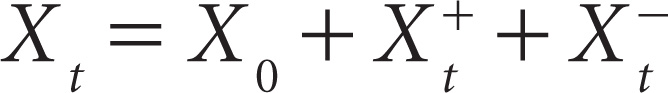
Thus, the cointegration function for the relationship between Y and X is the following:

Y_{t} = a + β^{+} X_{t}^{+} + β^{-} X_{t}^{-} + u_{t}

(6)

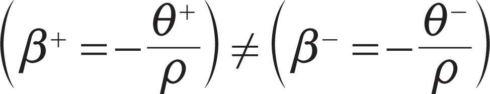
where u_t represents the error limit in this equation by mean value zero and fixed variance, while both β^– and β⁺ represent associated asymmetric long-term parameters.

$X_{t}^{+}$ and $X_{t}^{-}$ are calculated as in the following two equations:

X_{t}^{+} = \sum_{j = 1}^{t} Δ X_{j}^{+} = \sum_{j = 1}^{t} \max (Δ X_{j}, 0)

(7)

X_{t}^{-} = \sum_{j = 1}^{t} Δ X_{j}^{-} = \sum_{j = 1}^{t} \min (Δ X_{j}, 0)

(8)

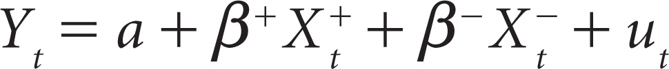
Based on that dividing of the explaining variable, inserting both $X_{t}^{+}$ and $X_{t}^{-}$ instead of X_t in ARDL model, we have NARDL model as follows:

\begin{matrix} Δ y_{t} = μ - ρ y_{t - 1} + θ^{+} x_{t - 1}^{+} + θ^{-} x_{t - 1}^{-} + \sum_{j = 1}^{ρ - 1} a_{j} Δ y_{(t - j)} \\ + \sum_{j = 0}^{q - 1} (π_{j}^{+} Δ x_{t - j}^{+} + π_{j}^{-} Δ x_{t - j}^{-}) + ε_{t} \end{matrix}

(9)

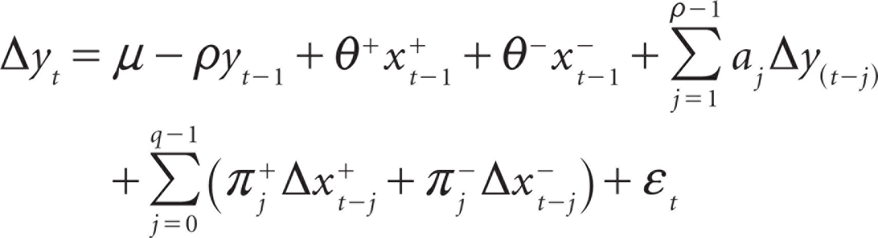
As in the previous model presented in Equation (1), θ⁺ & θ^– represents the long-term information of the asymmetric relationship in the model, and $π_{j}^{+} & π_{j}^{-}$ represent the asymmetric parameters in the long term.

Diagnostic tests of the NARDL model are similar to those of the ARDL model, where the cointegration is tested as in the following equation:

μ = ρ = θ^{+} = θ^{-} = 0

(10)

in addition to the normality distribution test of the error limit and model stability by using the cumulative sum test and CUSUM of squares test in addition to the heteroscedasticity test and error limit independence.

The advantage of the NARDL approach is the presence of an additional test, the symmetry test in the long term, where the following null hypothesis is tested by using the standard Wald test:

(β^{+} = - \frac{θ^{+}}{ρ}) = (β^{-} = - \frac{θ^{-}}{ρ})

(11)

opposite to the alternative hypothesis, which provides for the asymmetry of the relationship between the two variables of the study as follows:

(β^{+} = - \frac{θ^{+}}{ρ}) \neq (β^{-} = - \frac{θ^{-}}{ρ})

(12)

Accepting the null hypothesis and considering that the relationship is symmetric means that the relationship between the two variables is a linear relationship. Refusing the null hypothesis means accepting that the relationship between the two variables is nonlinear.

Linearity in the long term is tested by using the standard Wald test as follows:

\sum_{j = 0}^{q - 1} π_{j}^{+} = \sum_{j = 0}^{q - 1} π_{j}^{-}

(13)

3.3 Study Data

The Egyptian economy belongs to the lower-middle-income category, where the average individual share of the gross domestic product (GDP) is 2,645 dollars at fixed prices during the period 2010–2017. The Egyptian economy suffers from the problem of increasing internal and external debt. The central bank of Egypt estimated that the internal debt was 91 per cent of GDP in the financial year 2016–2017 and decreased to 83 per cent (3.1 trillion pounds) in the financial year 2017–2018. On the other hand, the Egyptian economy realizes good economic growth rates during the years 2010–2017. In accordance with the data provided by the World Bank, the average growth rate in real GDP per capita is 3.3 per cent during the period 2008–2017. Consumption is one of the most important drivers of economic growth in Egypt. The rate of consumption spending to GDP was (74.6%) in 2010 and grew to 82.4 per cent in 2015 then to 88.1 per cent in 2017. Accordingly, changes in this spending reflect strongly on GDP. Consumption spending depends on many sources; the most important ones are worker incomes in the economic sectors and money transfers by the Egyptian workers abroad, especially from the Arab Gulf countries. Total remittances were 9.8 billion dollars in 2010, which increased to 19.3 billion in 2015. Relatively, these transfers increased from 4.5 per cent to 5.8 per cent of GDP between 2010 and 2015, respectively (Helmy et al., 2017, p. 3).

In general, the Egyptian economy with its characteristics fits well in the group of developing or lower-middle-income economies.

In this study, the World Bank data set was used for the purpose of testing its main hypothesis for the period from 1970 to 2017. The governmental and consumption spending data were obtained at 2010 constant prices in the US dollars; also in constant prices, the national income was considered a variable representing disposable income because data for the latter are not available. The consumer price index (CPI) in 2010 equalled 100. The wealth variable is expressed by the broad money supply M2 as a proxy of the wealth.

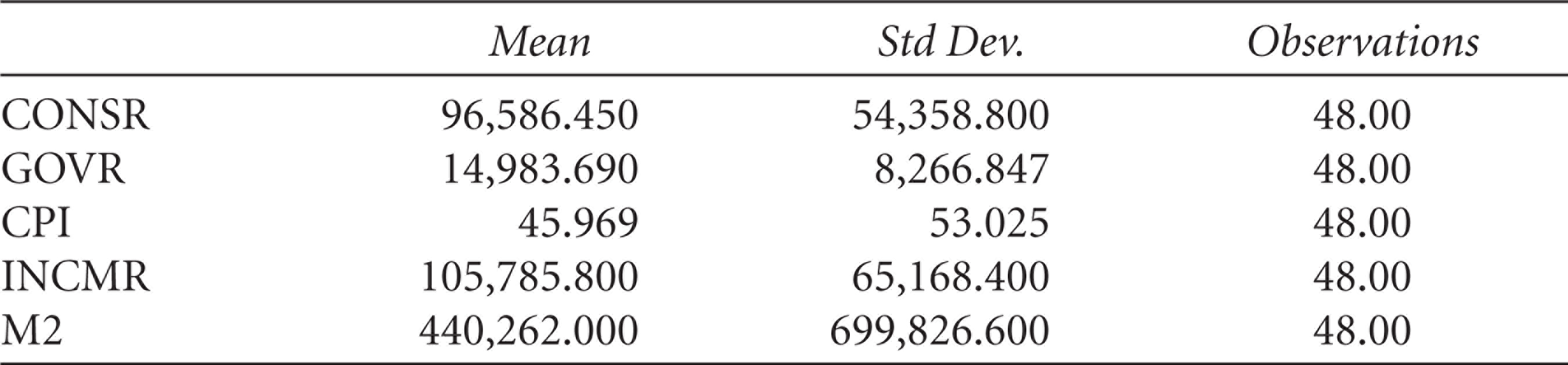
Table 1 presents the statistical characteristics of the data in the level. The results clarify that mean consumption spending is 96,586 million dollars in constant prices. Mean governmental spending was 14,983 million dollars in constant prices. On the other hand, mean national income was 105,785 million dollars in constant prices, and its mean wealth (measured by M2) is 440,262 million dollars in constant prices.

Figure 1 also shows the progress of all these variables during the study period after taking their natural logarithms.

Table 1
Statistical Characteristics of the Data

Mean Std Dev. Observations

CONSR 96,586.450 54,358.800 48.00

GOVR 14,983.690 8,266.847 48.00

CPI 45.969 53.025 48.00

INCMR 105,785.800 65,168.400 48.00

M2 440,262.000 699,826.600 48.00

	Mean	Std Dev.	Observations
CONSR	96,586.450	54,358.800	48.00
GOVR	14,983.690	8,266.847	48.00
CPI	45.969	53.025	48.00
INCMR	105,785.800	65,168.400	48.00
M2	440,262.000	699,826.600	48.00

Source: The author.

Figure 1

Source: Based on the author’s calculations from the World Bank data set.

4. Empirical Estimation and Results

4.1 Unit Root Test Results

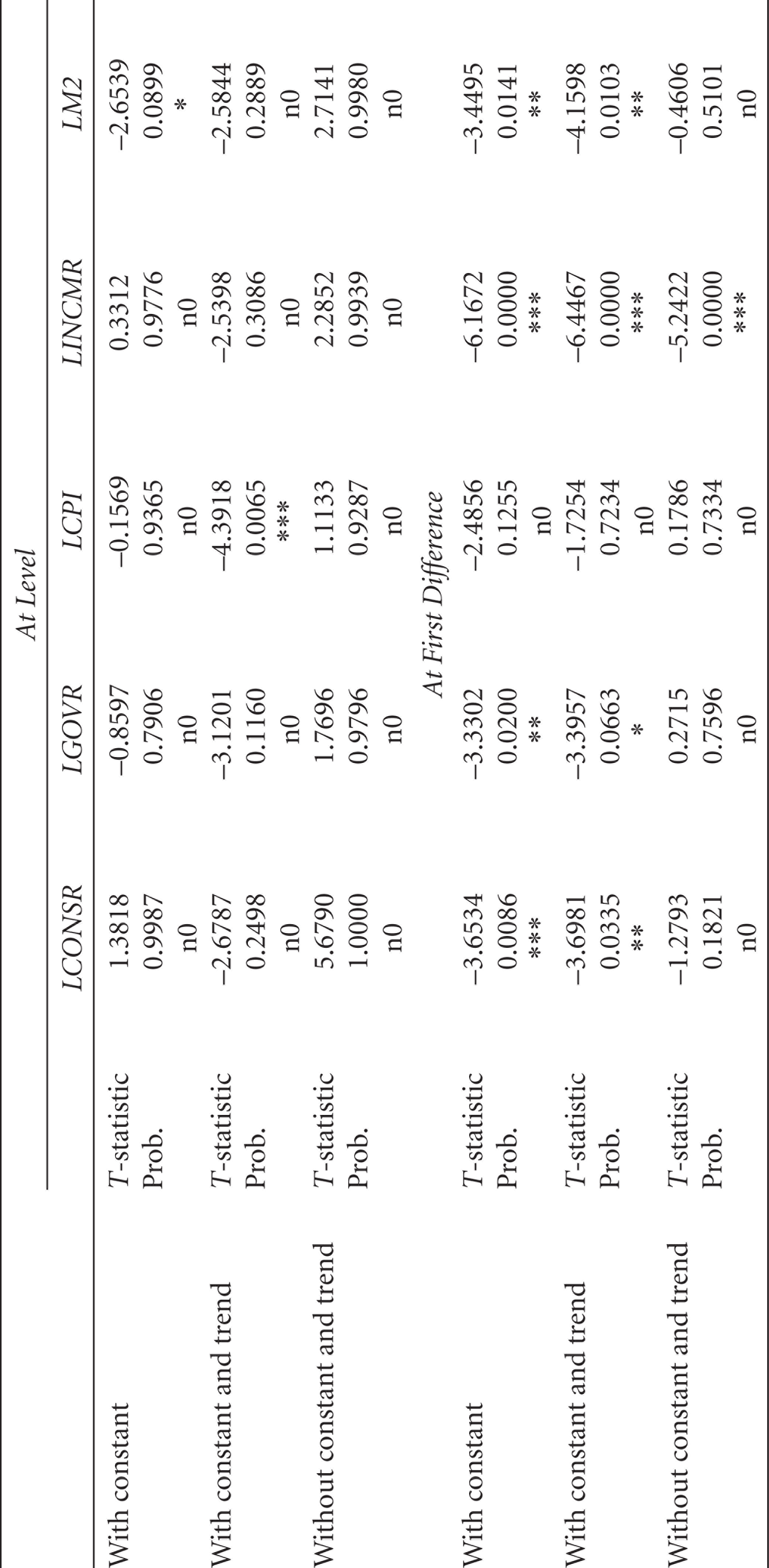
A unit root test is done to explore additional statistical characteristics of the time series and to identify the proper method of estimating the study model. There are many tests that can be used in this context. The test used in the study is the augmented Dicky–Fuller (ADF) test.

Table 2 includes results of the unit root test for the model data from using the ADF test. The results show that no variables are stationary at the level except LCPI, while the other variables have become stationary at the first difference. In other words, all of them (except CPI) have a unit root and integration of order I(1).

Table 2
Results of Unit Root Test from Using ADF

At Level

LCONSR LGOVR LCPI LINCMR LM2

With constant T-statistic 1.3818 –0.8597 –0.1569 0.3312 –2.6539

Prob. 0.9987 0.7906 0.9365 0.9776 0.0899

n0 n0 n0 n0 *

With constant and trend T-statistic –2.6787 –3.1201 –4.3918 –2.5398 –2.5844

Prob. 0.2498 0.1160 0.0065 0.3086 0.2889

n0 n0 *** n0 n0

Without constant and trend T-statistic 5.6790 1.7696 1.1133 2.2852 2.7141

Prob. 1.0000 0.9796 0.9287 0.9939 0.9980

n0 n0 n0 n0 n0

At First Difference

With constant T-statistic –3.6534 –3.3302 –2.4856 –6.1672 –3.4495

Prob. 0.0086 0.0200 0.1255 0.0000 0.0141

* n0 *

With constant and trend T-statistic –3.6981 –3.3957 –1.7254 –6.4467 –4.1598

Prob. 0.0335 0.0663 0.7234 0.0000 0.0103

** * n0 *

Without constant and trend T-statistic –1.2793 0.2715 0.1786 –5.2422 –0.4606

Prob. 0.1821 0.7596 0.7334 0.0000 0.5101

n0 n0 n0 *** n0

	At Level
With constant	T-statistic	1.3818	–0.8597	–0.1569	0.3312	–2.6539
	Prob.	0.9987	0.7906	0.9365	0.9776	0.0899
		n0	n0	n0	n0	*
With constant and trend	T-statistic	–2.6787	–3.1201	–4.3918	–2.5398	–2.5844
	Prob.	0.2498	0.1160	0.0065	0.3086	0.2889
		n0	n0	***	n0	n0
Without constant and trend	T-statistic	5.6790	1.7696	1.1133	2.2852	2.7141
	Prob.	1.0000	0.9796	0.9287	0.9939	0.9980
		n0	n0	n0	n0	n0
	At First Difference
With constant	T-statistic	–3.6534	–3.3302	–2.4856	–6.1672	–3.4495
	Prob.	0.0086	0.0200	0.1255	0.0000	0.0141
		***	**	n0	***	**
With constant and trend	T-statistic	–3.6981	–3.3957	–1.7254	–6.4467	–4.1598
	Prob.	0.0335	0.0663	0.7234	0.0000	0.0103
		**	*	n0	***	**
Without constant and trend	T-statistic	–1.2793	0.2715	0.1786	–5.2422	–0.4606
	Prob.	0.1821	0.7596	0.7334	0.0000	0.5101
		n0	n0	n0	***	n0

Source: The author.

Notes: ***, ** and * significant at 0.01, 0.05 and 0.10 levels, respectively.

Table 3

Unit Root Test Results from Using the Zivot and Andrews (1992)

Variables	Break in	T-statistic	Prob.	Breakpoint
LCONSR	Trend	–2.5123	0.0000	2003
LGOVR	Intercept	–0.8636	0.007	2009
LCPI	Intercept and trend	–0.5721	0.003	2010
LINCMR	Trend	–1.8212	0.0026	2005
LM3	Trend	–2.6894	0.0002	2010

Source: The author.

On the other hand, stationarity of the time series was tested by hypothesizing that there are structural breakpoints by using the Zivot and Andrews (1992) test. Table 3 shows the results of this test. These results show that the dependent variable (natural logarithm of governmental spending, LCONSR) had a structural transform in 2003, while that transform happened in 2009 for LGOVR and happened in 2005 concerning the CPI and in 2010 concerning the LM2.

Differences in the order stationary of the variables becoming drives us to use the ARDL approach for exploring the presence of a cointegration relationship between them and estimating the long-term relationship. Accordingly, we use the NARDL approach for testing the hypothesis of the (a)symmetric relationship between consumption and governmental spending in Egypt in the long term and the short term. The presence of a structural breakpoint in the dependent variable makes it proper to consider that breakpoint when estimating the study model.

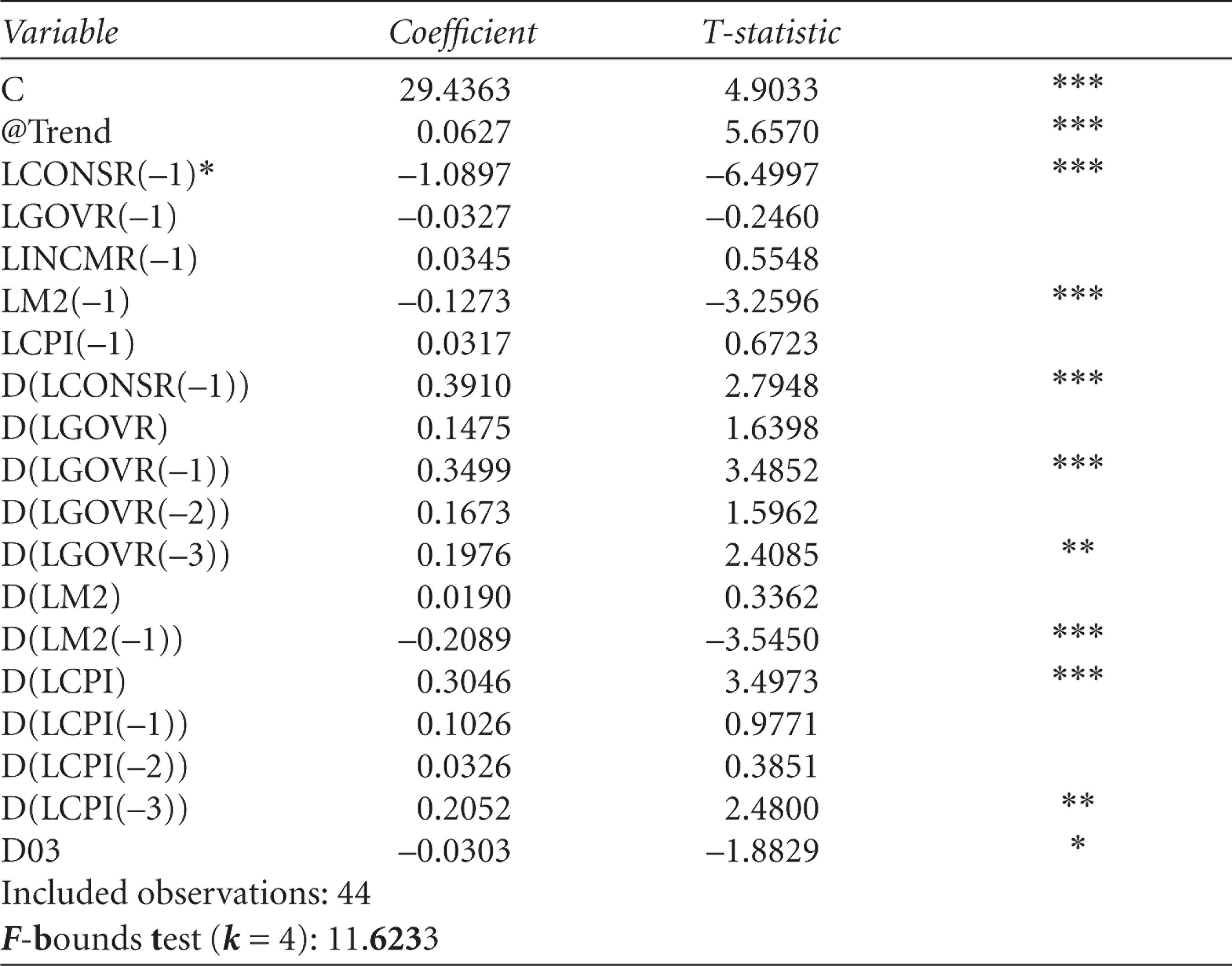
4.2 Empirical Results of The ARDL for the Bound Testing Model

Table 4 shows the results of estimating the study model using the ARDL approach, where Equation (4) was estimated. When taking into consideration the results of the Zivot and Andrews (1992) test, which shows that there is a structural breakpoint in the dependent variable in 2003, a dummy variable (D₀₃) was included the estimation equation where the variable is zero for the period 1970–2003 and one for the period 2004–2017.

The presented results show that the ECT is –1.0897, and it is significant at 1 per cent by using the critical value of the t-bound test from Pesaran et al. (2001; see Table A1). This result means that the model corrects the short-term errors towards the long term within approximately one year and that there is a cointegration critical value of the t-bound test from Pesaran et al. (2001).

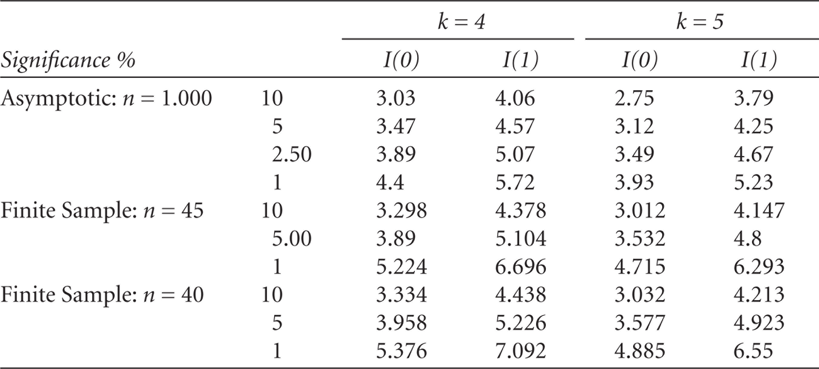
The results also show that the F-bound test is greater than the value of upper bound I(1) at 1 per cent significance level suggested by Narayan and Popp (2010) for 45 observations that equal 6.696 and 7.092 for 40 observations. This result means that the model reflects a cointegration relationship from the explaining variables to the dependent variable and enhances the result, which we concluded by using the t-bound test.

Table 4
Results of Estimating the Study Model

Variable Coefficient T-statistic

C 29.4363 4.9033 *

@Trend 0.0627 5.6570 *

LCONSR(–1)* –1.0897 –6.4997 *

LGOVR(–1) –0.0327 –0.2460

LINCMR(–1) 0.0345 0.5548

LM2(–1) –0.1273 –3.2596 *

LCPI(–1) 0.0317 0.6723

D(LCONSR(–1)) 0.3910 2.7948 *

D(LGOVR) 0.1475 1.6398

D(LGOVR(–1)) 0.3499 3.4852 *

D(LGOVR(–2)) 0.1673 1.5962

D(LGOVR(–3)) 0.1976 2.4085

D(LM2) 0.0190 0.3362

D(LM2(–1)) –0.2089 –3.5450 *

D(LCPI) 0.3046 3.4973 *

D(LCPI(–1)) 0.1026 0.9771

D(LCPI(–2)) 0.0326 0.3851

D(LCPI(–3)) 0.2052 2.4800

D03 –0.0303 –1.8829 *

Included observations: 44
F -bounds test ( k = 4): 11.6233

Variable	Coefficient	T-statistic
C	29.4363	4.9033	***
@Trend	0.0627	5.6570	***
LCONSR(–1)*	–1.0897	–6.4997	***
LGOVR(–1)	–0.0327	–0.2460
LINCMR(–1)	0.0345	0.5548
LM2(–1)	–0.1273	–3.2596	***
LCPI(–1)	0.0317	0.6723
D(LCONSR(–1))	0.3910	2.7948	***
D(LGOVR)	0.1475	1.6398
D(LGOVR(–1))	0.3499	3.4852	***
D(LGOVR(–2))	0.1673	1.5962
D(LGOVR(–3))	0.1976	2.4085	**
D(LM2)	0.0190	0.3362
D(LM2(–1))	–0.2089	–3.5450	***
D(LCPI)	0.3046	3.4973	***
D(LCPI(–1))	0.1026	0.9771
D(LCPI(–2))	0.0326	0.3851
D(LCPI(–3))	0.2052	2.4800	**
D03	–0.0303	–1.8829	*
Included observations: 44 F -bounds test ( k = 4): 11.6233

Source: The author.

Notes: ***, ** and * refer to significance levels of 1%, 5% and 10%, respectively.

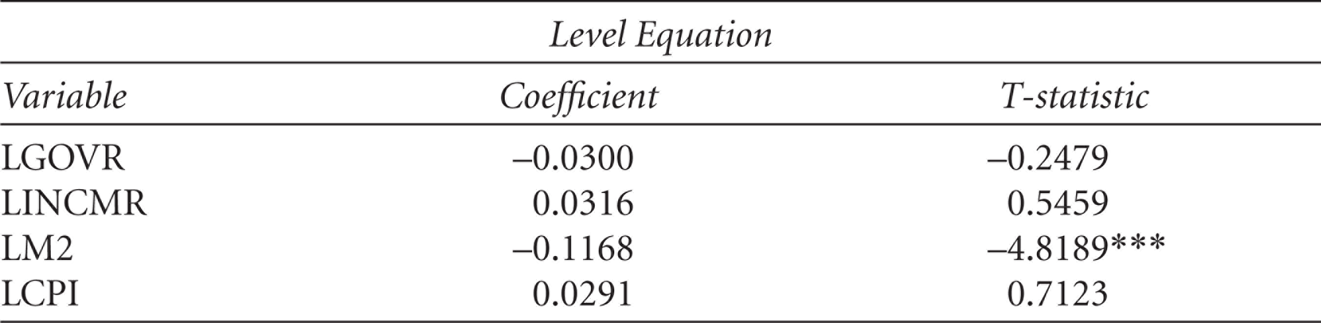
Table 5 shows the results of estimating the long-term parameters calculated in accordance with the equation $β_{n} = - \frac{λ_{n}}{λ_{0}}$ . Results of the significance of these parameters show that no parameters are significant except the parameter of the variable LM3 at 1 per cent. On the other hand, this parameter is negative. This result means that an increase in wealth identified by M3 leads to a decrease in consumption, which can be explained by that M3 increase, including different forms of savings, that was at the expense of consumption spending in Egypt, whereas an increase of M3 by 1 per cent will reduce consumption spending by 0.11 per cent. The results also show that government spending does not significantly affect consumption spending in Egypt.

Table 5

Long-term Estimators for the ARDL Model

Level Equation
Variable	Coefficient	T-statistic
LGOVR	–0.0300	–0.2479
LINCMR	0.0316	0.5459
LM2	–0.1168	–4.8189***
LCPI	0.0291	0.7123

Source: The author.

Notes: *** refers to the significance level of 1%.

Table 6

Results of the Diagnostic Tests for the ARDL Model

	Jarque–Bera (JB)	LM Test (F)	Heteroskedasticity (F)	Ramsey RESET Test (F)
Statistics	2.077	1.4567	0.8803	0.671
Prob.	0.354	0.2392	0.6038	0.421

Source: The author.

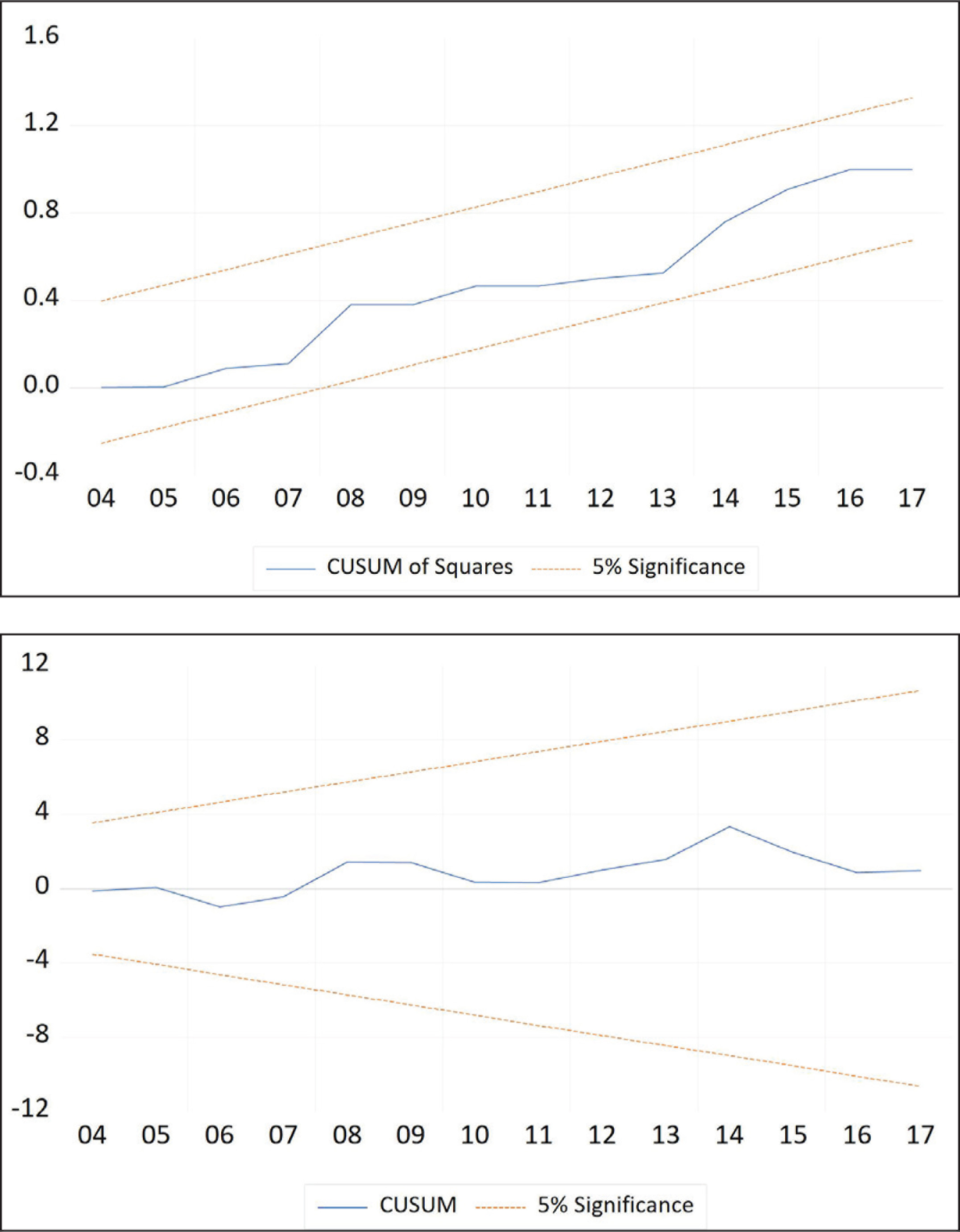
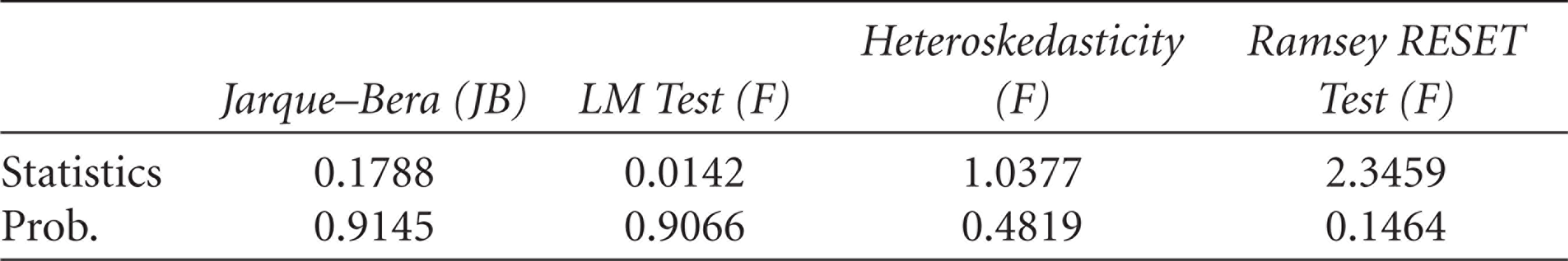
From the diagnostic aspect, Table 6 presents the results of the diagnostic tests for the estimated model. As the results show, the model does not have econometric problems. The residuals are normally distributed (by using the Jarque–Bera test), and they do not suffer from the serial autocorrelation problem (based on the LM test) or the problem of Heteroskedasticity (based on the Breusch-Pagan-Godfrey test). The results show that the model is proper concerning the functional form (based on the Ramsey RESET Test). Figure 2 presents the structural stability of the model, either at the level of the constant, depending on the CUSUM test, or at the level of the other parameters, depending on the CUSUMQ test. However, the critical bounds imply that the regressions are stable at 5 per cent significance level.

4.3 Empirical Results of the NARDL Model

Table 7 presents the results of estimating the NARDL model. The most important point revealed by these results is that the ECT is significant at less than 1 per cent by using the t test and by using the t-bound test. The critical value of the t-bound test, based on Pesaran et al. (2001), is –5.13, which is at a significance level of less than 1 per cent for five explanatory variables (k = 5; see Table A2). On the other hand, the result means that where λ = –1.47, that any shock will be overcome after less than one year, specifically within 8.16 months (approximately 8 months and 5 days). The results of this table show that the dummy variable (D₀₃) parameter was significant at 1 per cent, proving again that the year 2003 had a structural breakpoint in consumption spending in Egypt. The time parameter (Trend) was also significantly positive. This result shows that there is an increasing time trend in Egyptian consumption spending.

Figure 2

Source: The author.

One of the most important results is that of the bound test of cointegration (using the F-bound test). The results indicate a rejection of the null hypothesis and acceptance of the alternative hypothesis that there is a cointegration relationship and that the long-term parameters differ from zero.

Table 7

Results of Estimating the Study Model NARDL

Variable	Coefficient	T-statistic
C	33.0605	6.6601 ***
@Trend	0.0953	7.1983 ***
LCONSR(–1)	–1.4699	–7.1863 ***
LGOVR_POS(–1)	–1.2787	–5.3288 ***
LGOVR_NEG(–1)	–0.1864	–0.4184
LINCMR(–1)	0.2752	3.5166 ***
LM2(–1)	0.0355	0.8513
LCPI(–1)	0.0785	2.3211 **
D(LCONSR(–1))	0.2921	2.7425 **
D(LCONSR(–2))	0.3772	3.6142 ***
D(LCONSR(–3))	0.2789	3.5908 ***
D(LGOVR_POS)	–0.1989	–1.6257
D(LGOVR_POS(–1))	0.8285	3.8101 ***
D(LGOVR_POS(–2))	0.8231	9.8166 ***
D(LGOVR_POS(–3))	0.4795	3.0298 ***
D(LGOVR_NEG)	1.3330	2.0642 *
D(LGOVR_NEG(–1))	1.4144	3.6114 ***
D(LGOVR_NEG(–2))	–1.6244	–4.9605 ***
D(LGOVR_NEG(–3))	–1.4661	–2.3457 **
D(LINCMR)	0.1674	3.0688 ***
D(LINCMR(–1))	–0.1341	–2.7858 **
D(LM2)	0.1047	2.6821 **
D(LCPI)	–0.0680	–1.1588
D(LCPI(–1))	–0.1337	–1.9977 *
D(LCPI(–2))	–0.1004	–1.8859 *
D(LCPI(–3))	–0.1306	–2.2114 **
D ₀₃	–0.0306	–3.4375 ***
Included observations: 43 F-bounds test (k = 4): 11.4342

Source: The author.

Notes: ***, ** and * refer to significance levels of 1%, 5% and 10%, respectively.

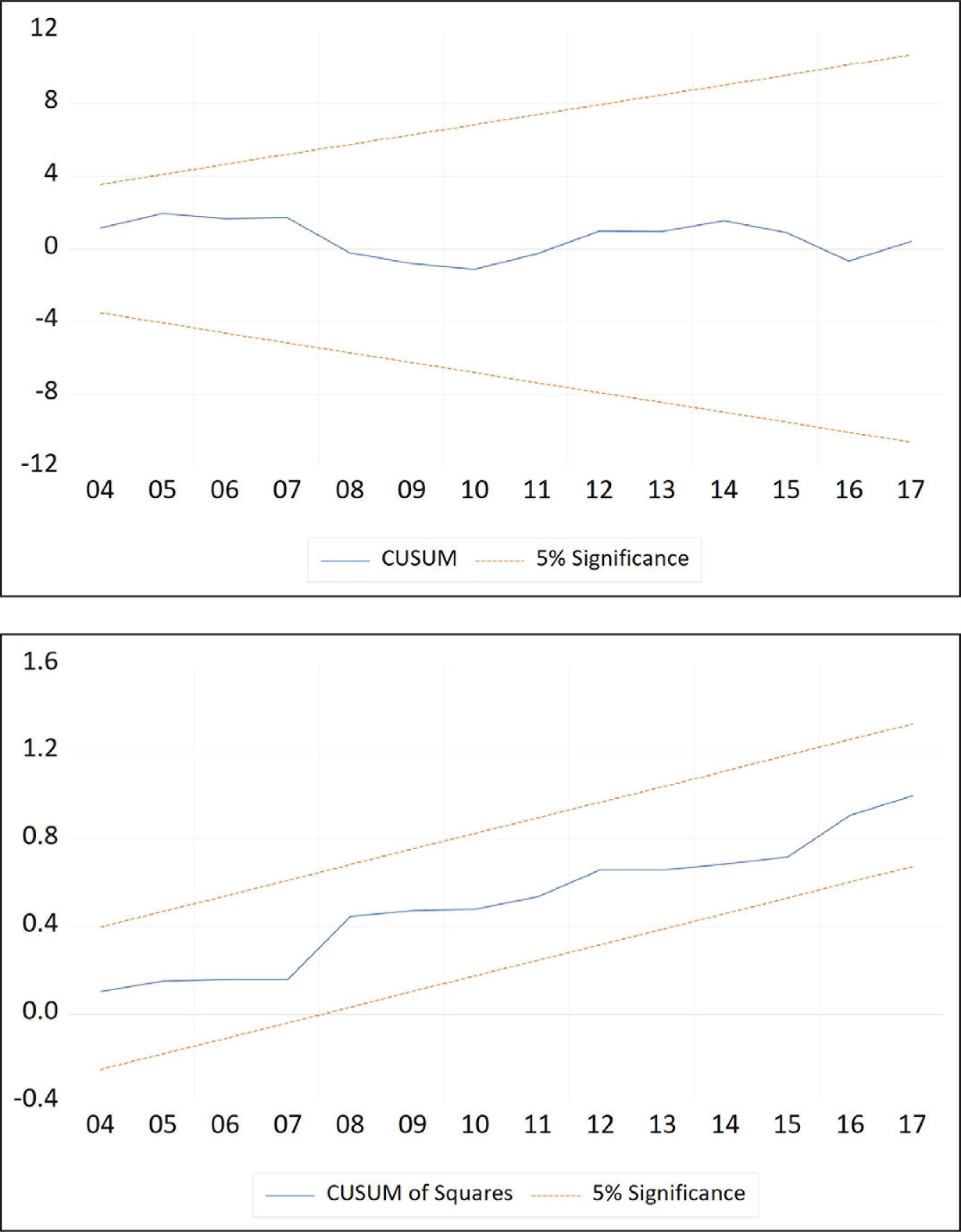
Table 8 shows that the model is free of residual problems. Based on the Jarque–Bera (JB) test, the results show that the residuals are normally distributed. Based on the LM test, the model does not suffer from an autocorrelation problem. The results also show that we accept the null hypothesis, which says that the variance of the error term is homoscedasticity (H₀: Homoscedasticity) based on the Breusch–Pagan–Godfrey test. The model is also correctly specified in general accordance with the Ramsey RESET test. Probability values show that the null hypotheses are accepted (H₀: Model is correctly specified). Figure 3 shows that the model is structurally stable either for the constant, using the CUSUM test, or for constancy of the coefficients in a model reflected by the CUSUM of squares test, whereas the plot which represents the two tests falls within the critical bound of 5 per cent.

Table 8

Results of the Diagnostic Test for the NARDL Model

	Jarque–Bera (JB)	LM Test (F)	Heteroskedasticity (F)	Ramsey RESET Test (F)
Statistics	0.1788	0.0142	1.0377	2.3459
Prob.	0.9145	0.9066	0.4819	0.1464

Source: The author.

Table 9

Results of Symmetry Tests in the Long Term and Short Term

(A)symmetric Test
	Long Term	Short Term
F-statistic	6.4610	3.1421
Prob.	0.0218	0.0953

Source: The author.

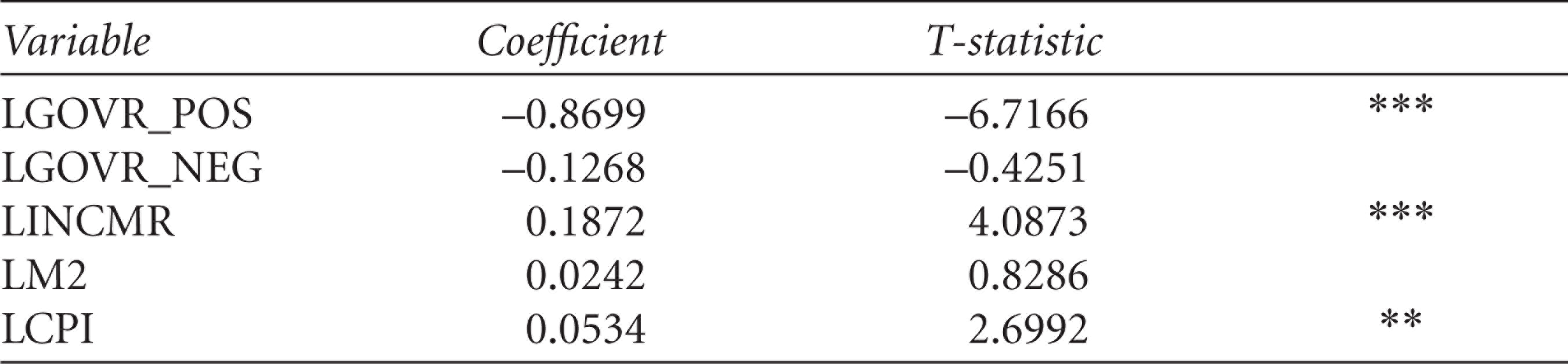
The results in Table 9 related to the symmetry test reveal that the calculated test statistics based on Equation (11) concerning the long term are greater than the critical value and that the probability value is less than 5 per cent. In other words, we reject the null hypothesis and accept the alternative hypothesis, which says that the long-term parameters are not equal. Thus, the relationship from governmental spending to consumption spending is asymmetric. The presence of the asymmetric relationship means that the effect of the positive values of governmental expenditure differs from the effect of negative value; the effect of an increase in government expenditure on consumer spending differs from the impact of a decrease in government spending on consumer spending. Returning to Table 10, the results indicate that the positive value parameter is significant at less than 1 per cent, while the negative value parameter is not significant.

The results in Table 10 show that a 1 per cent increase in government spending will result in a reduction in consumer spending by 0.8699 per cent. This result reveals that the relationship between the two types of spending is crowded out. Increased government spending requires more taxes at the cost of reducing consumer spending, which accounts for the bulk of national income. Whereas the average propensity to consume (APC) of a majority of the Egyptian population is almost equal to (1), based on the study database, tax deductions will be at the expense of consumption spending. The results of Table 10 indicate that the effect of national income is direct on consumption spending and significant at an elasticity coefficient 0.18. There is also a direct relationship from the CPI to consumption spending at 5 per cent significance level with an elasticity coefficient of 0.0534 per cent.

Table 10

Long-term Coefficients for the NARDL Model

Variable	Coefficient	T-statistic
LGOVR_POS	–0.8699	–6.7166	***
LGOVR_NEG	–0.1268	–0.4251
LINCMR	0.1872	4.0873	***
LM2	0.0242	0.8286
LCPI	0.0534	2.6992	**

Source: The author.

Note: ***, and ** refer to significance levels of 1, and 5%, respectively.

Figure 3

Source: The author.

5. Summary and Conclusion

The aim of this article is to test for the presence of a symmetric relationship directing from governmental spending to consumption spending in Egypt. The study used data covering the period from 1970 to 2017; these data were obtained from the World Bank data set published on the internet. Concerning the applied aspect, the study runs two tests. The first is a cointegration test on consumption function by using the ARDL approach, which involves many explanatory variables including the governmental spending. The results revealed that t-bound and F-bound tests refer to the presence of a long-term or cointegration relationship. However, exploring the effect of governmental spending on growth revealed that there is no long-term effect on consumption from governmental spending. The second test was run to complete the research on the nature of the relationship after dividing the effect of governmental spending into positive and negative values. This test was run by using the NARDL approach. The results revealed that the relationship is asymmetric between governmental spending and consumption. Consequently, there are different effects of the positive and negative governmental shocks. This result provides applied evidence of the research hypothesis, which says that the relationship between the two variables is not linear. The research results provide empirical evidence that the relationship between governmental and consumption spending is a crowd-out relationship, at least for developing countries represented well by the Egyptian economy. This result is in agreement with Bailey (1971), Ho (2001), Bouakez and Rebei (2007) and (Kwan, 2006). The substitutability coefficient was –0.8699 in the case of the positive shocks from governmental spending.

Footnotes

Declaration of Conflicting Interests

The author declared no potential conflicts of interest with respect to the research, authorship and/or publication of this article.

Funding

The author received no financial support for the research, authorship and/or publication of this article.

Appendix Tables

Table A2

Table Values of the F-bound Test for Explaining Variables 4 and 5 and in the Case of the Model Bound by the Time and Constant (Case No. 5)

Significance %		k = 4		k = 5
Significance %		I(0)	I(1)	I(0)	I(1)
Asymptotic: n = 1.000	10	3.03	4.06	2.75	3.79
	5	3.47	4.57	3.12	4.25
	2.50	3.89	5.07	3.49	4.67
	1	4.4	5.72	3.93	5.23
Finite Sample: n = 45	10	3.298	4.378	3.012	4.147
	5.00	3.89	5.104	3.532	4.8
	1	5.224	6.696	4.715	6.293
Finite Sample: n = 40	10	3.334	4.438	3.032	4.213
	5	3.958	5.226	3.577	4.923
	1	5.376	7.092	4.885	6.55

Source: Concerning the table values approximate to the sample from 1,000 observations from Pesaran et al. (2001). Concerning the table values for 40 and 45 observations from Narayan and Popp (2010).

References

Bailey

M. J.

(1971). National income and the price level: A study in macroeconomic theory. University of Michigan, McGraw-Hill.

Barro

R. J.

(1981). Output effects of government purchases. Journal of political Economy, 89(6), 1086–1121.

Baxter

, & King

R. G.

(1993). Fiscal policy in general equilibrium. The American Economic Review, 83(3), 315–334.

Bernardini

, & Peersman

(2018). Private debt overhang and the government spending multiplier: Evidence for the United States. Journal of applied econometrics, 33(4), 485–508.

Bouakez

, & Rebei

(2007). Why does private consumption rise after a government spending shock? Canadian Journal of Economics/Revue canadienne d’économique, 40(3), 954–979.

Coenen

, & Straub

(2005). Does government spending crowd in private consumption? Theory and empirical evidence for the euro area. International Finance, 8(3), 435–470.

D’Alessandro

(2010). How can government spending affect private consumption? A panel cointegration approach. European Journal Of Economics, Finance and Administrative Sciences, 18(18), 40–57.

Durkaya

(2012). The Relationship Between Public Expenditure and Private Consumption in Turkey(In Turkish). Maliye Dergisi, 163, 118–129.

Ercolani

, & Pavoni

(2012). The precautionary effect of government expenditures on private consumption. https://www.bancaditalia.it/pubblicazioni/altri-atti-seminari/2012/paper-Pavoni.pdf

10.

Evans

, & Karras

(1996). Private and government consumption with liquidity constraints. Journal of International Money and Finance, 15(2), 255–266. https://doi.org/10.1016/0261-5606(96)00006-X

11.

Graham

F. C.

(1993). Fiscal policy and aggregate demand: Comment. The American Economic Review, 83(3), 659–666.

12.

Granger

C. W.

, & Yoon

(2002). Hidden cointegration (Economics Working Paper [2002–02]). University of California.

13.

Hafedh

, & Nooman

(2007). Why does private consumption rise after a government spending shock? (Pourquoi est-ce que la consommation privée augmente après un choc de dépenses gouvernementales?). The Canadian Journal of Economics/Revue canadienne d’Economique, 40(3), 954–979.

14.

Helmy

, Zaki

, & Abdallah

(2017). Do workers’ remittances promote consumption stability in Egypt? The Egyptian Center for Economic Studies (ECES). http://www.eces.org.eg/PublicationsDetails?Lang=EN&C=12&T=1&ID=970&Do-Workers%E2%80%99-Remittances-promote-Consumption-Stability-in-Egypt?

15.

T-W.

(2001). The government spending and private consumption: A panel cointegration analysis. International Review of Economics & Finance, 10(1), 95–108.

16.

Khan

, Chen

, & Ashraf

(2015). Impact of government spending on private consumption using ARDL approach. Asian Economic and Financial Review, 5(2), 239–248.

17.

Kwan

Y. K.

(2006). The direct substitution between government and private consumption in East Asia. https://ideas.repec.org/p/nbr/nberwo/12431.html

18.

Narayan

P. K.

, & Popp

(2010). A new unit root test with two structural breaks in level and slope at unknown time. Journal of Applied Statistics, 37(9), 1425–1438.

19.

Pesaran

M. H.

, Shin

, & Smith

R. J.

(2001). Bounds testing approaches to the analysis of level relationships. Journal of Applied Econometrics, 16(3), 289–326.

20.

Samadi

A. H.

, & Sayedi

S. M.

(2012). Modeling the relationship between government expenditures and private consumption regarding the compensatory effects of government expenditures in Iran (1959–2007). Journal of Research in Economic Modeling, 2(8), 57–86.

21.

Shaikh

S. A.

(2018). An analysis of consumption function: A case study of upper middle income economies.

22.

Shin

, Yu

, & Greenwood-Nimmo

(2014). Modelling asymmetric cointegration and dynamic multipliers in a nonlinear ARDL framework. In Festschrift in honor of Peter Schmidt (pp. 281–314): Springer.

23.

Zivot

, & Andrews

D. W. K.

(1992). Further evidence on the great crash, the oil-price shock, and the unit-root hypothesis. Journal of business & economic statistics, 10(1), 251–270.

Is the Relationship Between Government Spending and Private Consumption in Egypt Symmetric?

Abstract

Keywords

1. Introduction

2. Theoretical Framework and Previous Studies

3. Study Model, Estimation Method, Study Data

3.1 Study Model

Table 1 Statistical Characteristics of the Data Mean Std Dev. Observations CONSR 96,586.450 54,358.800 48.00 GOVR 14,983.690 8,266.847 48.00 CPI 45.969 53.025 48.00 INCMR 105,785.800 65,168.400 48.00 M2 440,262.000 699,826.600 48.00

4.1 Unit Root Test Results

Footnotes

Declaration of Conflicting Interests

Funding

Appendix Tables

References

Table 1
Statistical Characteristics of the Data

Mean Std Dev. Observations

CONSR 96,586.450 54,358.800 48.00

GOVR 14,983.690 8,266.847 48.00

CPI 45.969 53.025 48.00

INCMR 105,785.800 65,168.400 48.00

M2 440,262.000 699,826.600 48.00