An Investigation into the Intertemporal Spending Path of Local Government in Mauritius

Abstract

This article examines whether local government expenditure in Mauritius is characterised by an intertemporal decision-making path. In other words, to what extent does local government expenditure respond to contemporaneous changes in revenues. In this respect, the article contributes to the existing body of literature by exploring the context of an upper-middle-income country like Mauritius while factoring intertemporal choice in the supply of local public goods. Moreover, the article determines the short-run and long-run responsiveness of local public expenditure to Gross Domestic Product (GDP) through an error correction model based on time series data for Mauritius over the period 1987–2017. Our findings indicate that local government spending becomes less sensitive to its previous values when GDP and its past values are introduced as control variables in the model. Local government expenditure and real output are also found to be co-integrated or to share a long-term relationship.

JEL Classification: B22, C1, D9, H4, H11

Keywords

Local government expenditure Intertemporal spending Mauritius Cointegration GDP growth Error correction model Time series

1. Introduction

Intertemporal choices are fundamental to any decision-making in the world of economics, since they relate to the present and future as in intertemporal savings–investment choices whereby the individual chooses how much to consume today and how much to save for future consumption. These theoretical explanations date back to the pioneering works of Ramsey (1928) and Fisher’s (1930) two-period general intertemporal optimisation in his Theory of Interest and form the cornerstone of growth models as the Solow growth model (Solow, 1956) and the Ramsey-Cass-Koopman neoclassical economic growth models (Cass 1965). As such, government spending and investment decision by analogy is an intertemporal choice as to how much to spend today, tax and how much to spend tomorrow or intertemporally in infinite period settings. Such local expenditure for local government pertains to investment that brings a return in the future in the form of higher economic growth, through improved infrastructure as emphasised by the endogenous growth models of Barro (1990) and King and Rebelo (1990), which predict long-run growth rates based on productive expenditures. Although intertemporal decisions involve trade-offs across periods so that costs and benefits are spread over time, a recurring argument in economic theory is that social welfare is optimised when a benevolent government can commit intertemporally. Irrespective of jurisdictions or political systems, governments face a common need to govern for the future, but a range of policy issues from climate change to ageing population and debt sustainability confront them with an intertemporal dilemma: maximising present social welfare or caring for the future. As put forward by Jacobs (2016), for democratic governments, this choice becomes an even more thorny political predicament when the benefits of costly policies only show up after the next election (Jacobs, 2016).

During the last decade, a number of studies have examined intertemporal models based on rational forward-looking behaviour (Borge & Tovmo, 2018; Borge et al., 2001; Holtz-Eakin, 1993; Holtz-Eakin et al., 1989; Jacobs, 2016; Legrenzi & Milas, 2011). While intertemporal decision-making models have been employed with some success to analyse the fiscal behaviours of federal governments, they have also yielded mixed results. Some studies indicate that government behaviour is characterised by a longer-term decision-making horizon (Dahlberg & Lindström, 1998; Holtz-Eakin & Rosen, 1993; Rattsø, 1999), and, in many countries, this tendency for forward decision-making was prompted by the consecutive deregulation of financial markets and other economic transformations that mitigated the importance of current revenues for local spending (Dahlberg & Lindström, 1998).

The primary purpose of this article is therefore to offer a simple framework for verifying if local government expenditure¹ is generated by the maximisation under uncertainty of an intertemporal utility function, using times-series data for Mauritius for the period 1987–2017. In other words, it examines the extent to which local spending can be rationalised by an error correction model (ECM) in which decisions are based on permanent rather than current levels of resources available to the local sector. The article is organised as follows: Section 2 presents the intertemporal model of government expenditure to be estimated. Section 3 explains the data and local context, followed by Section 4 that sets the econometric methodology, namely, the three alternative approaches used for testing for co-integration between real local government expenditure and real GDP. Section 5 presents the empirical findings of the Engle and Granger procedure (Engle & Granger, 1987), the Johansen approach (Johansen, 1988) and the Gregory–Hansen (Gregory & Hansen, 1996) test for co-integration in the presence of a structural break under the autoregressive distributed lag (ARDL) framework (Pesaran & Shin, 1996). Section 6 concludes with a discussion of the results and some suggestions for future research.

2. An Intertemporal Model of Local Government Spending

Almost any choice can be rationalised through utility functions. Where decisions involve streams of receipts and payments as in the case of any government with taxes and other incomes on the one hand and expenditures on the other, some testable solutions can be identified for more meaningful conclusions. The central planner is assumed to be a forward-looking agent who derives utility through local government spending² and maximises an intertemporal utility function in the presence of a budget constraint. We assume that the central government derives satisfaction in devolution that is by promoting decentralisation. The function is specified as follows where the central planner maximises expected discounted sum of utility as in Equation 1,

E_{t} \sum_{ƒ = 0}^{T - 1} {(1 + δ)}^{- τ} U (L G_{t + τ})

(1)

which is subject to its budget constraint,

\sum_{τ = 0}^{T - 1} {(1 + r)}^{- τ} (L G_{t + τ} + C G_{t + τ}) = R_{t}

(2)

Where, E_t is the expectation conditional on available information at time t; δ is a social rate of discount (different from the market rate of interest); r is real rate of interest (r ≥ δ), assumed constant over time; T is time horizon; U is a concave instantaneous or one period utility function; LG_t is local government expenditure; CG_t is central government expenditure; and R_t is revenue of the central government.

The revenue of the central government of Mauritius as defined by Statistics Mauritius comprises mainly of taxes (income tax paid by individuals and companies; VAT; and excise duties on a number of products including alcoholic beverages, motor vehicles, petroleum products and others); social contributions by employers and employees for pensions and other social security schemes; grants representing transfers from other levels of government, foreign governments and international organisations; and property income including interest, dividends and fines among others.

We solve this problem by using Lagrange multipliers. The Lagrange multiplier is λ and the Lagrangean expression (Equation 3) is considered.

L = E_{t} \sum_{τ = 0}^{T - 1} {(1 + δ)}^{- τ} U (L G_{t + τ}) + ª \sum_{τ = 0}^{T - 1} {(1 + r)}^{- 1} (L G_{t + τ} + C G_{t + τ}) - R_{t}

(3)

Analysing the intertemporal choice exercise over two periods, the central planner faces the following first-order condition in Period 1:

U^{'} (L G_{t}) + ª = 0

such that,

λ = - U^{'} (L G_{t})

(4)

In Period 2, we have the following first-order condition:

[U^{'} (L G_{t + 1}) {(1 + δ)}^{- 1}] + λ {(1 + r)}^{- 1} = 0

such that,

λ = - [U^{'} (L G_{t + 1}) {(1 + δ)}^{- 1}] (1 + r)

(5)

Equating (4) and (5), we have

U^{'} (L G_{t}) = [{(1 + δ)}^{- 1} (1 + r)] (U^{'} [(L G_{t + 1}) = 0

Implying that

U^{'} [L G_{t}] (1 + δ) {(1 + r)}^{- 1} = U^{'} (L G_{t + 1})

(6)

Equation 6 is the usual intertemporal margin which balances present and future local government expenditure and indicates that the government is indifferent about small changes in local government expenditure across any two time periods.

A quadratic concave (additive over time) function is considered as follows:

U (L G_{t}) = - \frac{1}{2} [{(W - L G_{t})}^{2}

(7)

with W representing an ensured minimum utility level.

Therefore, the intertemporal choice of local government expenditure can be shown to work as follows over the two periods:

W - L G_{t} = {(1 + δ)}^{- 1} (1 + r) {W - (L G_{t + 1})}

(8)

Solving for LG_t+1, we have

L G_{t + 1} = α_{0} + α_{1} (L G_{t})

(9)

Where the constant term

α_{0} = W [1 - (1 + δ) {(1 + r)}^{- 1}]; α_{1} = [(1 + δ) {(1 + r)}^{- 1}]

Equation 9 is lagged by one period:

L G_{t} = α_{0} + α_{1} L G_{t - 1}

(10)

Equation 10 constitutes a random walk with drift. One can establish whether local government spending is carried out on a systematic basis (where the coefficient of α₁ is significantly different from zero and less than unity) or random basis (where the coefficient of α₁ is insignificant).

In Equation 11, we introduce real GDP (GDP_t) as an exogenous variable in the model as well as its lagged value in order to test the intertemporal decision-making of the government. Since by inspecting both local government expenditure and output are non-stationary variables, we proceed to establish both a long-run and short-run relationship/s among the variables.

L G_{t} = ψ + ψ_{1} G D P_{t} + ψ_{2} L G_{t - 1} + ψ_{3} G D P_{t - 1} + u_{t}

(11)

Taking the log of Equation 11 and treating small letter cases as log, we have

\lg_{t} = ψ + ψ_{1} G D P_{t} + ψ_{2} \lg_{t - 1} + ψ_{3} G D P_{t - 1} + u_{t}

(12)

Subtracting lg_t–1 on both sides and adding ψ₁ GDP_t and subtracting ψ₁ GDP_t on the RHS yields:

Δ \lg_{t} = ψ + (ψ_{2} - 1) (\lg_{t - 1} - \frac{ψ}{1 - ψ_{2}} - (\frac{ψ_{1} + ψ_{3}}{1 - ψ_{2}}) G D P_{t - 1}) + ψ_{1} Δ G D P_{t} + u_{t}

(13)

Having defined the theoretical underpinning of the above equation and its coefficients, the next step is to empirically test Equation 13 to verify whether central government in Mauritius has a systematic or random approach for allocating the local government budget.

Suppose lg_t and GDP_t are non-stationary (I(1)) variables and u_t is a stationary process (I(0)), then we see that only if $\lg_{t - 1} - \frac{ψ}{1 - ψ_{2}} - (\frac{ψ_{1} + ψ_{3}}{1 - ψ_{2}}) G D P_{t - 1}$ is I(0), can we have a valid relationship. This requires that lg_t and GDP_t be co-integrated.

Equation 13 is an ECM of the form below with (ψ₂ – 1) being replaced as λ

Δ y_{t} = \emptyset_{0} + \sum_{j = 1} \emptyset_{j} Δ y_{t - j} + \sum_{h = 0} \emptyset_{i} Δ x_{t - h} + λ E C T_{t - 1} + μ_{t}

(14)

3. Data and Local Context

The case of Mauritius is well suited for an analysis of intertemporal spending behaviour since it differs in some respect from many Scandinavian countries and aligns in some others with sub-Saharan African states in the way central government regulations of budgeting and borrowing influence local authorities’ intertemporal budget constraint. The general government sector in Mauritius is made up of the central government, the local government and, as from 2002, the regional government (which includes the administration of Rodrigues). The central government includes ministries, departments as well as agencies responsible for the effective delivery of specialised government functions in specific areas including health, education and social welfare among others. The Local Government Act, 2011 provides the legislative framework for a system of local government that enables local communities to manage their affairs through elected local authorities, which comprise municipalities and district councils. The Ministry of Local Government and Outer Islands is responsible for local government matters in Mauritius, and it oversees the local authorities and the legislative framework to ensure that they operate smoothly.

Our research focuses on the local government sector only and analyses the behaviour of local spending as measured by local government expenditure. The time series data for the period 1987–2017 are drawn from the Digest of Public Finance Statistics, which is an annual publication of the Statistics Mauritius, an official body responsible for the collection, analysis and dissemination of economic and social data for the island. Local government expenditure relates to the spending of the Ministry of Local Government and Outer Islands in various areas, including general public services, transport, environmental protection, housing and community amenities, recreation and culture and social protection among others. An estimate of this expenditure stood at Rs³ 4.3 billion in 2017 and has more than doubled over the last 10 years. This represents around 3.7 per cent of the consolidated general government expenditure⁴ for that year. A major share of this represents a grant-in-aid earmarked for the 12 municipalities and district councils of the island. As it is, in every financial year, the central government allocates a grant from the Consolidation Fund to the Ministry of Local Government, designated for the local authorities. The latter contributes around 65 per cent of the revenues of councils, which adds to their ‘own’ generated revenues in the form of trade fees from economic operators, rentals, fees from markets and fairs and from the issue of Building and Land Use Permits and general rates (raised by municipalities only). The grant-in-aid to local authorities has more than doubled since 2008 when it stood at around Rs1.8 billion and increased to about Rs2.8 billion in 2014 to reach approximately Rs4 billion in financial year 2017–2018.⁵ This is shared among municipalities and district councils on the basis of a pre-determined grant-in-aid formula that takes into consideration the financial and development needs of each local authority.

Institutional setting has a strong impact on the intertemporal spending behaviour of the government in Mauritius. The fact that local authorities are authorised to borrow, subject to the approval of the central government, for capital expenditures by way of debentures or bonds suggests that they can be forward-looking in their spending. The more so as they are also allowed, subject to central government’s approval and to some pre-defined extent, to incur expenditures during the year that were not included in their expenditure estimates (Local Government Act, 2011). However, there are budgetary restrictions as spelt out in the Local Government Act, 2011 to contain expenditures and borrowing within strict rules as the latter are subject to the approval of the minister for local government affairs. Moreover, fiscal policy formulation is set within a medium-term expenditure framework (MTEF) which takes into account the macroeconomic objectives and challenges of the government. Specific provisions on public finance are also made in the Constitution, which also allows for a Contingency Fund that authorises the minister responsible for finance to meet unforeseen and urgent expenditures for which provisions have not been made. Thus, although there is room for a forward-looking approach to government spending, there is always the basic requirement for prudential budgeting with adherence to the Finance and Audit Act, 2008 and the Public Debt Management Act, 2008, which defines the statutory debt ceiling for a particular fiscal year. There has been on several counts the need for bailouts from the central government in a few instances. In times of crisis or output shocks, it was justified to place some fiscal rules in line with providing countercyclical stimulus beyond the constraints for normal times. The local government has also on several occasions been confronted with the need for additional fiscal packages to local authorities to cater for emergencies where torrential rains, for instance, called for major capital investments in road and drains repairs and other capital projects.

Figure 1 is based on data pertaining to real GDP and real local government expenditure trends for Mauritius for the period 1987–2017, and these have been adjusted using the GDP deflator.⁶ The values have been compiled from the Digest of Public Finance Statistics which is an annual publication of Statistics Mauritius. All data comply with the Government Finance Statistics Manual 2001 (GFS)⁷ of the IMF (David & Petri, 2013). As seen in the time series plots, both variables are trending upwards with some more visible fluctuations in local government expenditure in specific years as compared to the smoother evolution of real GDP. Real GDP experienced a considerable and steady growth over the last 30 years from about Rs70 billion in 1987 to over Rs300 billion in 2017 (Statistics Mauritius, 2019a; Statistics Mauritius, 2019b).

Figure 1.

Source: Adapted from the Digest of Public Finance Statistics, Mauritius.

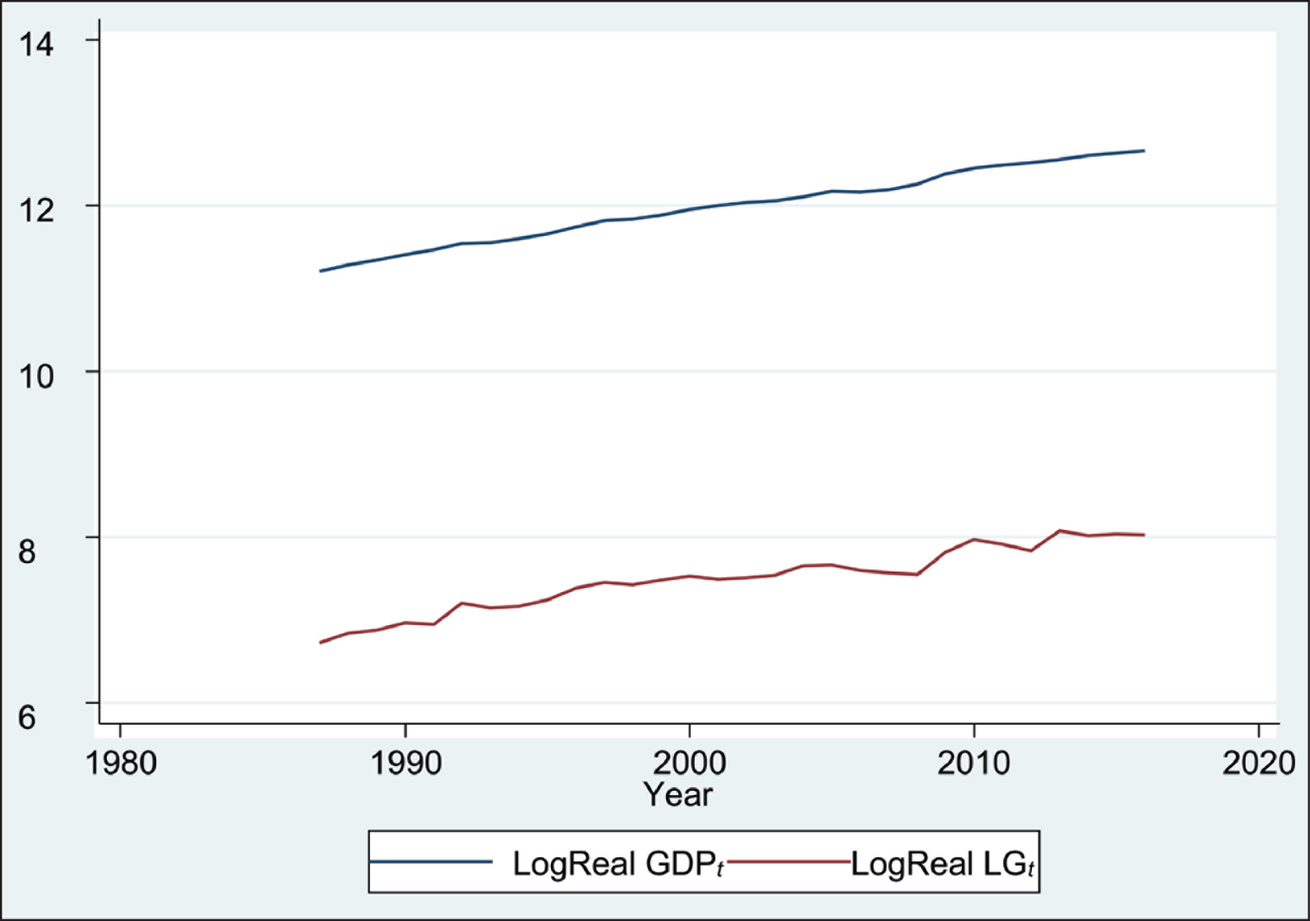
The past 30 years have been mostly characterised by political stability as well as a sound macroeconomic environment which has been sustained through a host of economic reforms.⁸ This has enabled the country to move successfully from a monocrop economy to a diversified services-based middle-income economy. The share of total government expenditure of GDP over this period has stagnated at around 25 per cent to reach 27 per cent in 2017, with exceptions in some years like 2007–2008 when it fell to 22 per cent of GDP. As a share of GDP, local government spending has remained relatively low, stagnating around 1 per cent of GDP and falling below that level from 2006 to 2008, and reached 0.97 per cent of GDP in 2017. Although both series show an increasing trend overtime, Figure 2 demonstrates that the fluctuations in real local government spending have been more acute compared with changes in real GDP with sharp increases in some years and drops in others.

Figure 2.

Source: Adapted from the Digest of Public Finance Statistics, Statistics Mauritius.

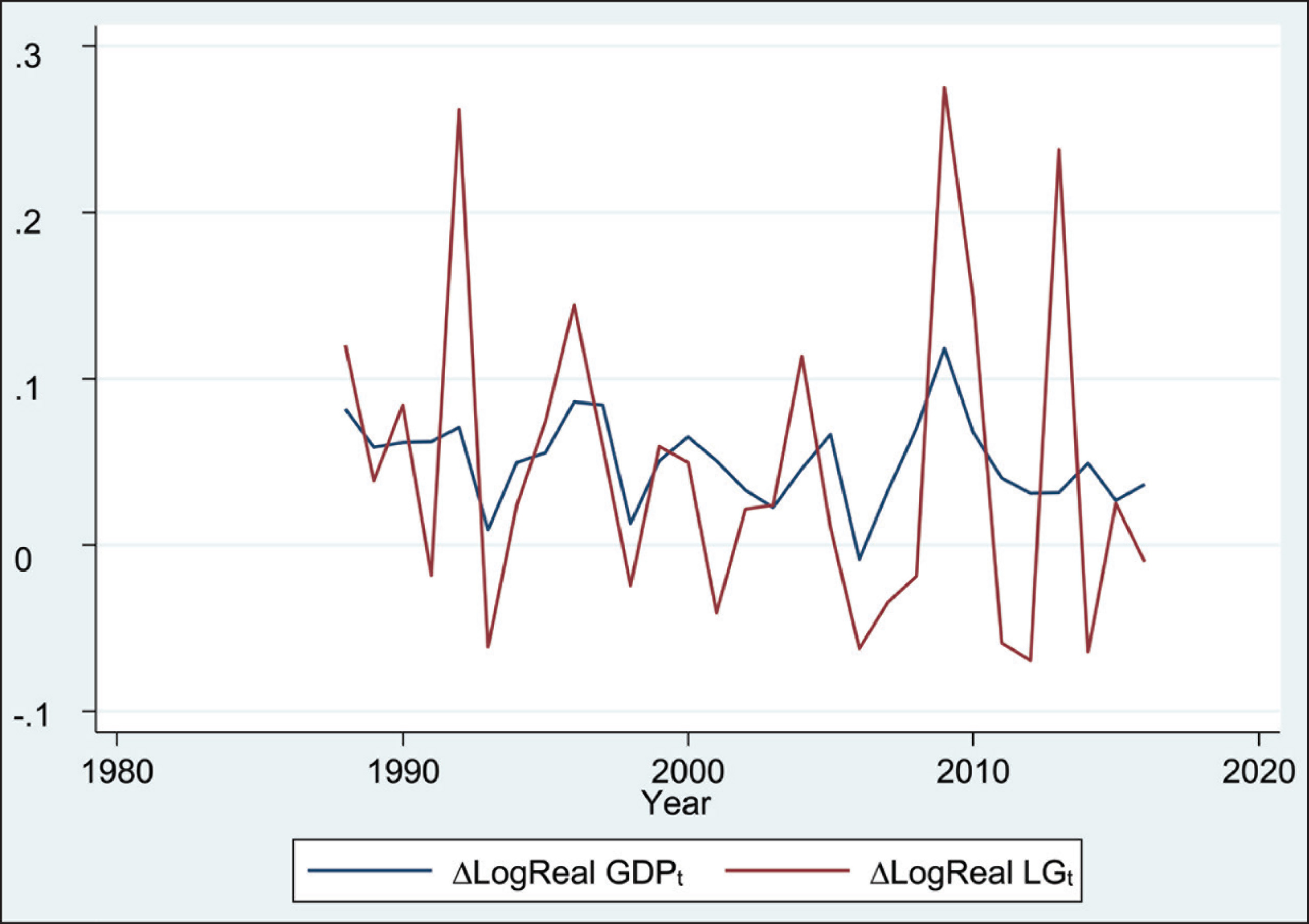
The years post 2000 marked a period of structural transformations following the phasing-out of textile trade preferences and the loss of sugar preferences (David & Petri, 2013). A decomposition of public expenditures over the past years also indicate that the share of current expenditures on total expenditure has increased more specifically from 2008–2009 due to counter-cyclical policies to mitigate the adverse effects of the global financial crisis. In fact, the share of expenditure on physical capital dropped both in relative terms and as a share of GDP. For some years, public expenditure has been quite volatile and current expenditures including transfers to local government dropped (David & Petri, 2013). It can be seen from Figure 3 that central government tax revenue by far exceeds local government revenue.

Figure 3.

Source: Adapted from the Digest of Public Finance Statistics, Statistics Mauritius.

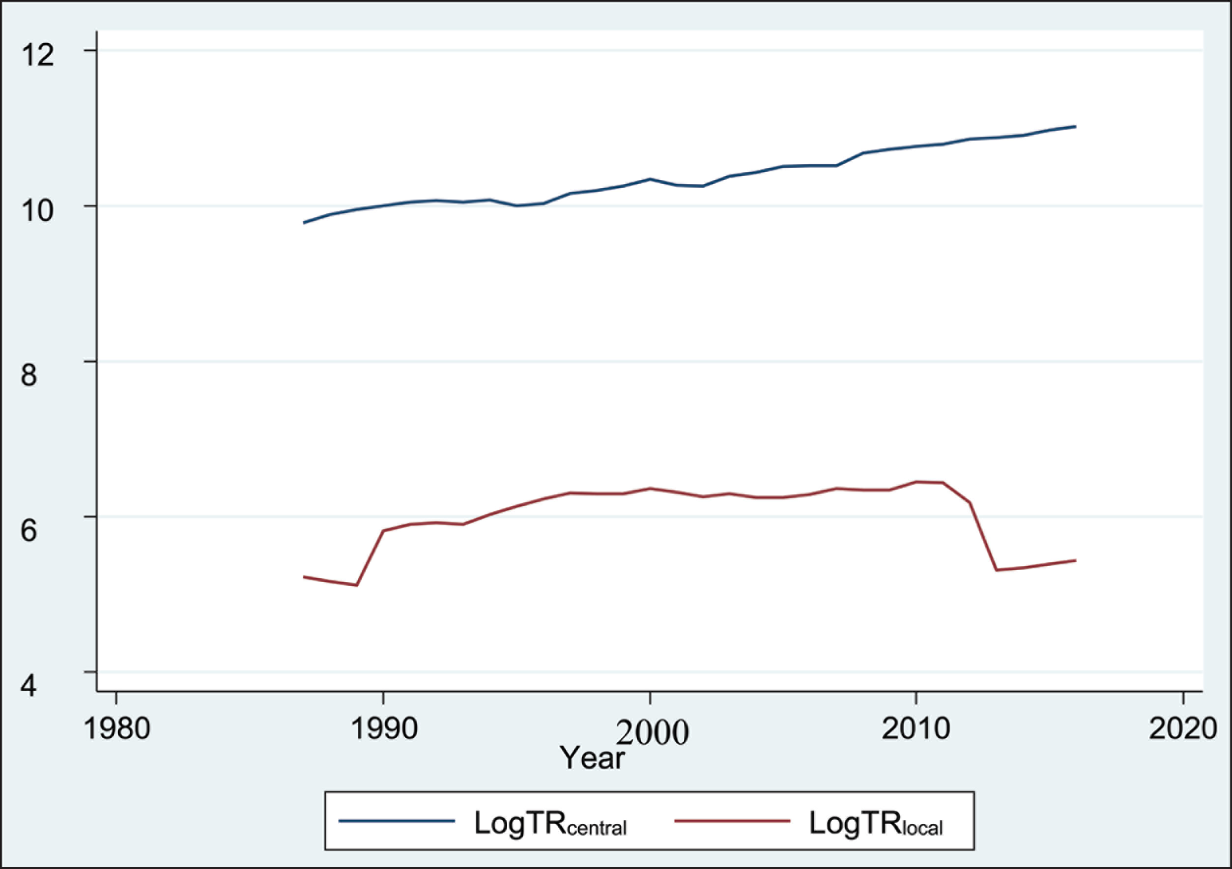
Local government taxes as a percentage of central government taxes averaged 1–2 per cent and fell to 0.4 per cent following the institution of the Mauritius Revenue Authority (MRA) when the administration of revenue collection was entrusted to semi-autonomous or parastatal bodies for enhanced revenue collection and trade facilitation.

4. Econometric Methodology

The empirical procedure adopted in this essay employs three approaches to study the presence of a long-term relationship between local expenditure and income in Mauritius. But prior to that, it was deemed relevant to investigate whether local government spending follows a random walk or is subject to excess smoothing. Accordingly, Equation 10 in the econometric model has been estimated in the first place to find out whether the coefficient of LG_t–1, that is α₁ is significantly different from zero and less than unity, which would indicate that the allocation of local government budgets are carried out on a systematic basis as opposed to an alternative scenario where it is exclusively random. This has been further evidenced by estimating Equation 12 to also assess the influence of real income on local government spending in the local context.

In order to test for cointegration between local government expenditure and real income, the Engle and Granger approach (Engle & Granger, 1987) has been used. Also, through the Johansen cointegration procedure (Johansen, 1988), which extends the single-equation ECM to a multivariate system, the ECM has been defined to determine the relationship between the variables. The specific merits of the ARDL approach (Pesaran & Shin, 1996), namely its appropriateness for small samples and potential for providing unbiased estimates of the long-run model even if one of the regressors is endogenous, have in addition been tapped by conducting the Gregory–Hansen (Gregory & Hansen, 1996; 2009) cointegration test in the presence of a structural break.

The notion of having recourse to co-integrating vectors in the study of non-stationary time series stems from the works of Granger (1981) and Engle and Granger (1987), and their linkages with ECMs, have been examined by a number of researchers (Johansen, 1988). Prior to estimating Equation 14, the Augmented Dickey Fuller (ADF) unit root test is performed to verify if the variables used in the model are stationary using Equation 11 for any time series Z_t where

Δ Z_{t} = \partial_{0} + \partial_{1} T + \geq γ_{1} Δ Z_{t - 1} + \geq γ_{2} Δ Z_{t - 2} + \dots + \geq γ_{k} Δ Z_{t - k} + u_{t}

(15)

∆Z_t-1 represents the lagged first-difference included in the equation to accommodate serial correlation in the errors. Equation 15 tests the null hypothesis of a unit root against a mean-stationary alternative in Z_t. Since a visual inspection of the times-series plots depicts upward trends over time for both Log Real GDP_t and Log Real LG_t and in order to control for serial correlation, the ADF test reports results with both a constant and a time trend included, respectively. In order to ensure that the residuals have normality properties, the tests of skewness and kurtosis have been carried out along with a test of no autocorrelation of the stochastic term using the Lagrange Multiplier statistics.

5. Econometric Results

This section analyses whether local government spending follows a random walk and is split into two.

5.1 Does Local Spending Follow a Random Walk?

Equation 10 introduced earlier is estimated as follows:

\begin{array}{l} L o g L_{t} = 0.58 + 0.93 L o g L_{t - 1} \\ \begin{matrix} \begin{matrix} \begin{matrix} \begin{matrix} \begin{matrix} \begin{matrix}  \end{matrix} \end{matrix} \end{matrix} \end{matrix} \end{matrix} & 19.51 (.000) \end{matrix} \end{array}

(10)

The results from the ARDL model of the form of Equation 12 are

\begin{array}{l} L o g L_{t} = - 1.58 + 1.57 L o g G D P_{t} + 0.41 L o g L_{t - 1} - 1.7 L o g G D P_{t - 1} \\ \begin{matrix} \begin{matrix} \begin{matrix} \begin{matrix} \begin{matrix} \begin{matrix} \begin{matrix} \begin{matrix} \begin{matrix} \begin{matrix}  \end{matrix} \end{matrix} \end{matrix} \end{matrix} \end{matrix} \end{matrix} \end{matrix} \end{matrix} \end{matrix} & 2.52 (.018) 2.81 (.009) 2.18 (.039) - 1.71 (0.099) \end{matrix} \end{array}

(12)

The above findings reveal that even when the model is extended to include real GDP and its lagged values, local government spending is still affected by its previous value, although the latter now exerts a weaker influence on current spending while real GDP produces a much stronger influence on it at the 1 per cent level of significance. This is explained by the fact that the budgetary allocation in the form of the grant-in-aid, which largely makes up LG_t in the model, is to a large extent determined by the amount of ‘own revenues’ that local authorities raise. A larger proportion of ‘own revenues’ in the form of fees, rates and rentals generated by councils should necessitate a lower central budgetary allocation for meeting local expenditures. The fact that these ‘own revenues’ are quite sensitive to the level of economic activity, including consumption and investment in the economy, makes the budgetary allocation for meeting local government expenditure dependent on real income. This can also be evidenced by the negative relationship between local spending in the current year and real GDP in the previous year, if this constitutes a lower revenue base for local councils thereby requiring a larger grant-in-aid in the following fiscal year to meet local expenditure.

5.2 Unit Root Test

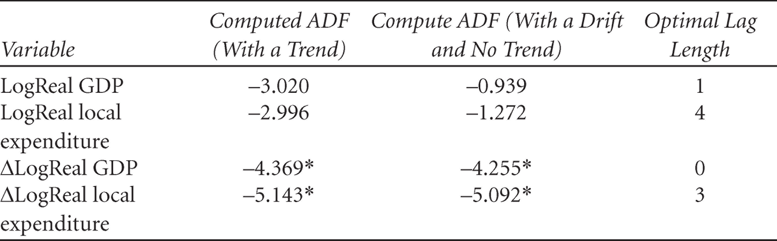
To test whether there is a long-term relationship between local government spending and GDP, we carry out the unit roots tests. The results of the ADF test with a trend, and with a drift and no trend, are reported in Table 1.

Table 1.
Unit Root Test of Variables

Variable Computed ADF (With a Trend) Compute ADF (With a Drift and No Trend) Optimal Lag Length

LogReal GDP –3.020 –0.939 1

LogReal local expenditure –2.996 –1.272 4

∆LogReal GDP –4.369* –4.255* 0

∆LogReal local expenditure –5.143* –5.092* 3

Variable	Computed ADF (With a Trend)	Compute ADF (With a Drift and No Trend)	Optimal Lag Length
LogReal GDP	–3.020	–0.939	1
LogReal local expenditure	–2.996	–1.272	4
∆LogReal GDP	–4.369*	–4.255*	0
∆LogReal local expenditure	–5.143*	–5.092*	3

Source: The authors.

Note: * indicates significance at 1 per cent level.

Table 1 shows that both the levels of Log Real GDP and Log Real Local Government Expenditure contain a unit root when the test is specified with a trend, and their first differences are stationary with the hypothesis of non-stationary being rejected at the 1 per cent level of significance. The variables are integrated of the same order, that is, they are both I(1), and the optimal lag length is determined by the relevant value of the Akaike Information Criterion (AIC).

5.3 The Engle and Granger Approach

Engle and Granger (1987) recommend a two-step approach for cointegration analysis. A long-run equilibrium equation is

\lg_{t} = ψ + ψ_{1} G D P_{t} + ψ_{2} \lg_{t - 1} + ψ_{3} G D P_{t - 1} + u_{t}

(16)

Where the OLS residuals from Equation 16 represent a measure of disequilibrium and a test of cointegration is a test of whether u_t is stationary. This is carried out by performing the ADF test on the residuals, with the Engle and Yoo (1987) critical values. If there is cointegration, the OLS estimator of Equation 16 is said to be super consistent, meaning that as T tends towards infinity, the need for I(0) variables in the co-integrating equation disappears.

A simple manipulation gives us the second step of the Engle and Granger ECM, which is as follows:

Δ \lg_{t} = ψ + (ψ_{2} - 1) (\lg_{t - 1} - \frac{ψ}{1 - ψ_{2}} - (\frac{ψ_{1} + ψ_{3}}{1 - ψ_{2}}) G D P_{t - 1}) + ψ_{1} Δ G D P_{t} + u_{t}

Δ \lg_{t} = \emptyset_{0} + λ (\lg_{t - 1} - \frac{ψ}{1 - ψ_{2}} - (\frac{ψ_{1} + ψ_{3}}{1 - ψ_{2}}) G D P_{t - 1}) + \emptyset_{i} Δ G D P_{t} + u_{t}

Adding few more dynamics and short-run relationships yield the following:

Δ y_{t} = \emptyset_{0} + \sum_{j = 1} \emptyset_{j} Δ y_{t - j} + \sum_{h = 0} \emptyset_{i} Δ x_{t - h} + λ E C T_{t - 1} + μ_{t}

(17)

Where $E C T_{t - 1} = \lg_{t - 1} - \frac{ψ}{1 - ψ_{2}} - (\frac{ψ_{1} + ψ_{3}}{1 - ψ_{2}}) G D P_{t - 1}$

OLS is used here as Equation 17 has only I = (0) variables, so that any standard hypothesis testing using t-statistics, including a diagnostic testing of the error term, is appropriate. The adjustment coefficient λ is expected to be negative. In short, the ECM describes how the variables under study behave in the short run, consistent with a long-run co-integrating relationship (Engle & Granger, 1987).

The relationship between local expenditure and real GDP is thus estimated using OLS, and the empirical results are summarised in Table 2.

L o g L G_{t} = - 2.78 + 0.86 \log {(G D P)}_{t} + u_{t}

It is noted that real GDP has a positive and significant relationship (p = .00) on real local expenditure.

Since the estimated u is based on the estimated co-integrating parameter δ₁, the Engle and Granger critical values are appropriate to use. In Table 2, the Engle and Granger (1987) computed ADF statistic of the residuals from a linear regression equation of LogL_t and LogGDP_t is –3.892 and significant at the 5 per cent level.

Table 2.

OLS Results

LogL_t	Coefficient	Std Error	t	p > \|t\|
LogGDP_t	0.86	0.032	26.97	0.00
_cons	–2.78	0.38	–7.31	0.00

Source: The authors.

Notes: F(1,28) = 727 (0.00); r-squared = 0.96; DW d-stat (2, 30) = 1.29

The conclusion from Table 3 is that the estimated u_t is stationary, meaning that it does not have a unit root, and real local expenditure and real GDP, despite being individually non-stationary, are co-integrated.

Table 3.

The Engle–Granger Test for Cointegration

Test Statistic	*1%	*5%	*10%
–3.892	–4.301	–3.555	–3.194

Source: The authors.

Note: *Critical values from Engle and Yoo (1987).

Figure 4 shows the time series plot of the residuals and Figure 5 is a plot of the residuals against their lagged values.

Figure 4.

Source: Adapted from the Digest of Public Finance Statistics, Statistics Mauritius.

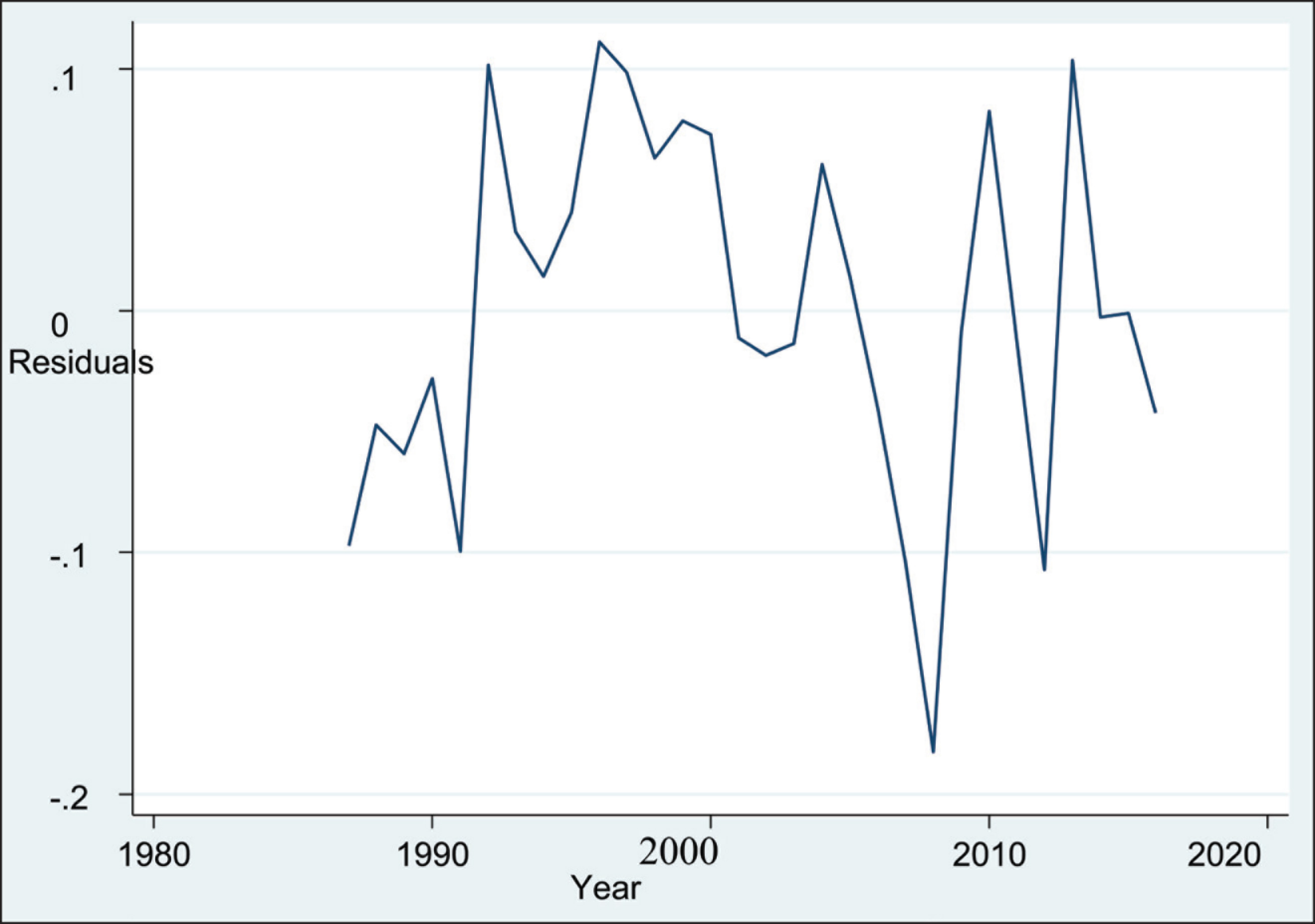
Since cointegration is not rejected, a dynamic ECM as specified in Equation 14 is estimated. The ECM provides a means for reconciling the short-run behaviour of the variables with their long-run behaviour (Engle & Granger, 1987).

As defined earlier, in a generalised version, the ECM can be stated as:

Δ y_{t} = \emptyset_{0} + \sum_{j = 1} \emptyset_{j} Δ y_{t - j} + \sum_{h = 0} \emptyset_{i} Δ x_{t - h} + λ E C T_{t - 1} + μ_{t}

(18)

Equation 18 relates the change in real local expenditure to the change in real GDP and the ‘equilibrating’ error in the previous period.

Even when the equation is specified with one lag only, the lagged differences of real local spending and real GDP do not produce any significant impacts on local spending as shown below.

Figure 5.

Source: Adapted from the Digest of Public Finance Statistics, Statistics Mauritius.

\begin{array}{l} Δ L o g L G_{t} = 0.81 {\hat{u}}_{t - 1} - 0.0087 Δ L o g L G_{t - 1} + 0.83 Δ L o g G D P_{t - 1} + 0.0049 \\ - 3.18 (0.004) - 0.04 (0.971) + 1.11 (0.279) + 0.14 (0.833) \end{array}

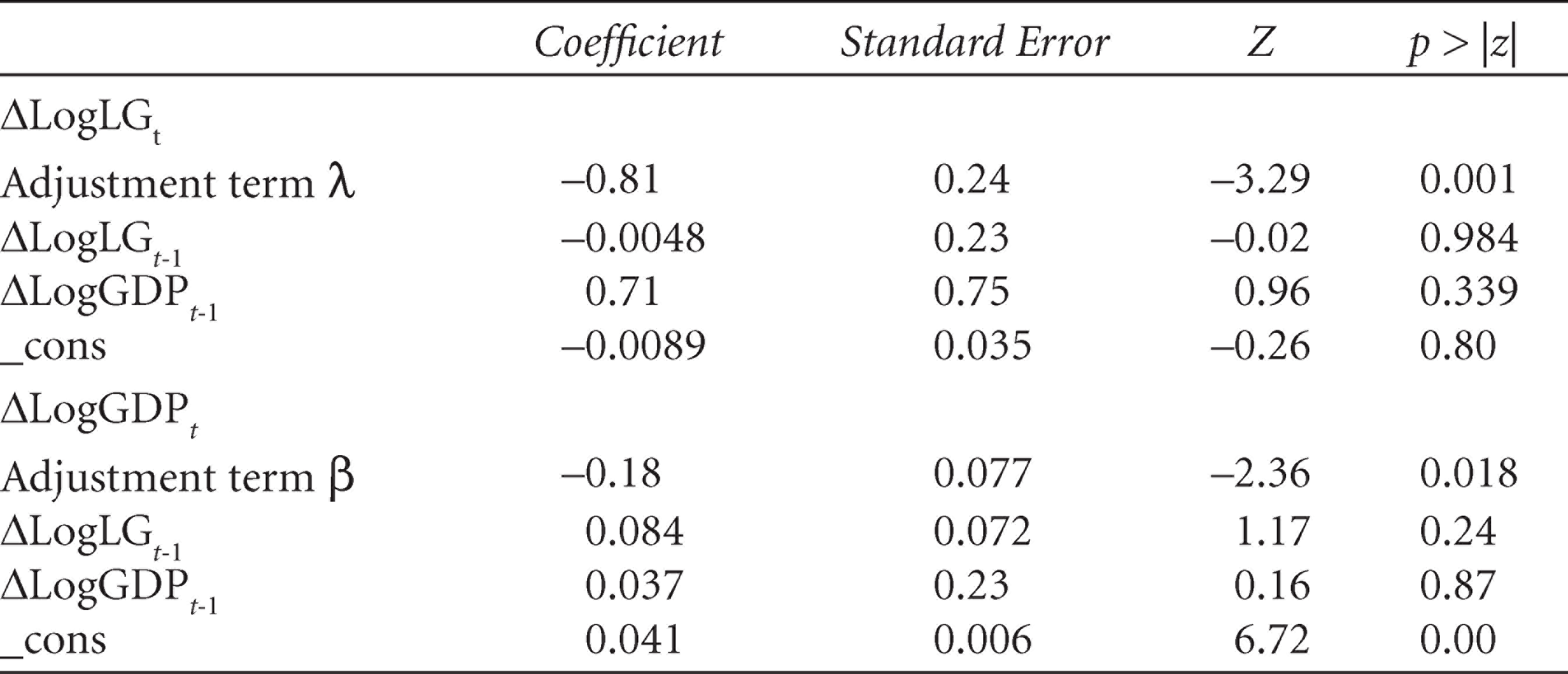
It is deduced that short-run changes in real GDP do not have significant effects on real local expenditure, but the latter adjusts to its long-run growth path fairly quickly following a disturbance, as depicted by the ECM parameter (–0.81) which is negative and significant at the 5 per cent level. The results convey that local government expenditure in Mauritius is in line with intertemporal decision-making, meaning that it is co-integrated with real output and that both variables share a long-term relationship. This is expected in the sense that if central government spends too much in one year, it has to contain its expenditure commitments in the next year in line with fiscal prudence and budget sustainability to contain the budget deficit to some 3 per cent and the public sector debt to around 60 per cent.

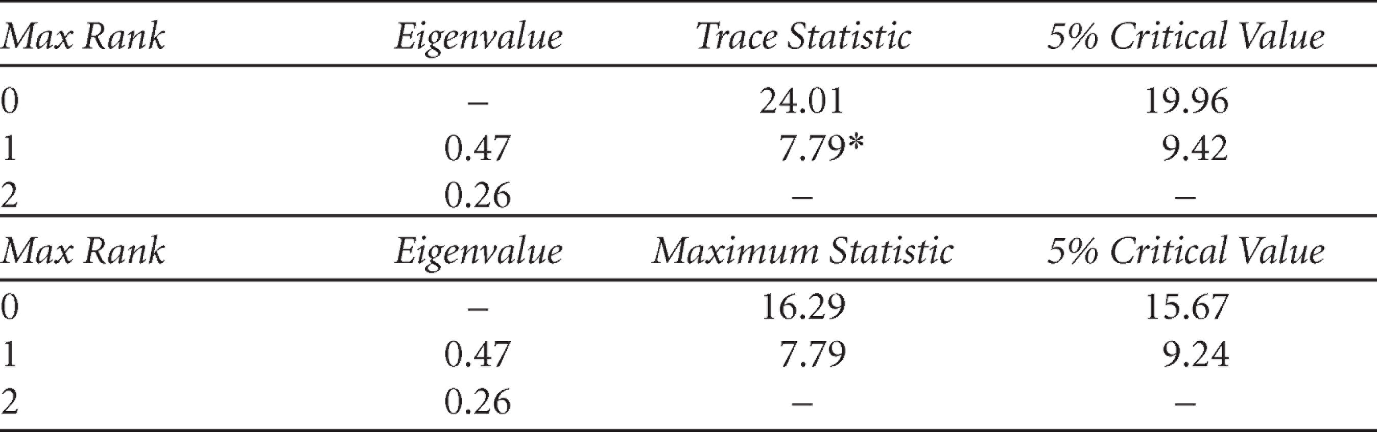
5.4 The Johansen Cointegration Test

As an alternative approach for testing for cointegration between the variables and stating their long-run relationship, the Johansen technique has also been employed (Johansen, 1988). When a restricted constant is specified, at maximum rank zero, the trace statistic (24.01) exceeds the 5 per cent critical value (19.96). The null hypothesis that there is no cointegration is thus rejected, suggesting that the time series variables LogLG_t and LogGDP_t are co-integrated with a maximum of one co-integrating vector. The maximum statistics conveys similar conclusions as reported in Table 4.

Table 4.
Johansen’s Test for Cointegration

Max Rank Eigenvalue Trace Statistic 5% Critical Value

0 – 24.01 19.96

1 0.47 7.79* 9.42

2 0.26 – –

Max Rank Eigenvalue Maximum Statistic 5% Critical Value

0 – 16.29 15.67

1 0.47 7.79 9.24

2 0.26 – –

Max Rank Eigenvalue Trace Statistic 5% Critical Value

0 – 24.01 19.96

1 0.47 7.79* 9.42

2 0.26 – –

Max Rank Eigenvalue Maximum Statistic 5% Critical Value

0 – 16.29 15.67

1 0.47 7.79 9.24

2 0.26 – –

Max Rank	Eigenvalue	Trace Statistic	5% Critical Value
0	–	24.01	19.96
1	0.47	7.79*	9.42
2	0.26	–	–
Max Rank	Eigenvalue	Maximum Statistic	5% Critical Value
0	–	16.29	15.67
1	0.47	7.79	9.24
2	0.26	–	–

Max Rank	Eigenvalue	Trace Statistic	5% Critical Value
0	–	24.01	19.96
1	0.47	7.79*	9.42
2	0.26	–	–
Max Rank	Eigenvalue	Maximum Statistic	5% Critical Value
0	–	16.29	15.67
1	0.47	7.79	9.24
2	0.26	–	–

Source: The authors.

Note: ** indicates significance at 1% level.

In a generalised version, the ECM can be stated as

E C T_{t - 1} = y_{t - 1} - \partial_{j} x_{t - 1}

where

E C T_{t - 1} = 1.000 L o g L G_{t - 1} - 0.81 L o g G D P_{t - 1} + 2.16

and

Δ L o g L G_{t} = - 0.0048 Δ L o g L G_{t - 1} + 0.71 Δ L o g G D P_{t - 1}^{}_{+}^{} - 0.81 E C T_{t - 1} - 0.0089

The estimation equation is

\begin{matrix} Δ L o g L G_{t} = - 0.0048 Δ L o g L G_{t - 1} + 0.71 Δ L o g G D P_{t - 1} - 0.81 E C T_{t - 1} + \\ 0.66 L o g G D P_{t - 1} - 1.76 \end{matrix}

(19)

As seen in Table 5, neither the lagged first differences of local government expenditure nor those of GDP produce any significant influence on the change in local spending in the short run. This is also true when the model is estimated with four lags. In the long run, real GDP has a positive impact on real local expenditure (the sign is reversed) and the coefficient of adjustment (–0.81) is significant at the 1 per cent level. This suggests that the previous years’ errors or deviations from long-run equilibrium are corrected for within the current year at a convergence speed of 81 per cent. Although this observation is beyond the scope of the research, it is useful to note that the lagged differences of real local expenditure and GDP do not produce any significant impact on the change in real GDP in the short run while the adjustment term β is also statistically significant at the 5 per cent level. However, real GDP takes longer to adjust to shocks in local spending given the very low share of local expenditure of GDP and the low multiplier effects of local government spending which is mostly limited to small infrastructural municipal projects.

Table 5.

Short-Run Coefficients

	Coefficient	Standard Error	Z	p > \|z\|
∆LogLG_t
Adjustment term λ	–0.81	0.24	–3.29	0.001
∆LogLG_t-1	–0.0048	0.23	–0.02	0.984
∆LogGDP_t-1	0.71	0.75	0.96	0.339
_cons	–0.0089	0.035	–0.26	0.80
∆LogGDP_t
Adjustment term β	–0.18	0.077	–2.36	0.018
∆LogLG_t-1	0.084	0.072	1.17	0.24
∆LogGDP_t-1	0.037	0.23	0.16	0.87
_cons	0.041	0.006	6.72	0.00

Source: The authors.

The Eigenvalue stability condition of the vector error correction model (VECM) has also been examined. The VECM has two endogenous variables and one co-integrating vector. There is a one-unit moduli in the comparison matrix, and no other remaining moduli computed is too close to one, which confirms the stationarity of the co-integrating equation.

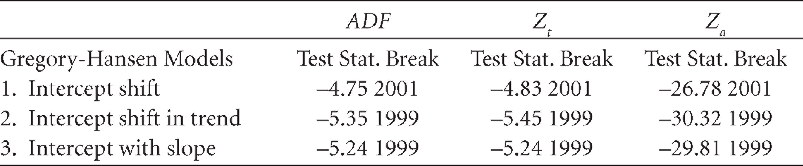
5.5 The Gregory Hansen Cointegration Test (with a Structural Break)

If the series are co-integrated but this linear combination has shifted at one point in time in the sample implying the possibility of a structural break, the standard tests for cointegration might not be appropriate, as highlighted by Gregory and Hansen (1996). This is because they only presume that the co-integrating vector is time invariant under the alternative hypothesis. Gregory and Hansen (1996) proposed extensions of the ADF, Z_α and Z_a tests for cointegration for a shift in either the intercept or the whole coefficient vector. Also the tests are non-informative of the timing of the structural break and therefore less likely to be contaminated by a break suggested merely by the visual examination of the time series (Gregory & Hansen, 1996). The Gregory–Hansen cointegration test confirms that there is no cointegration in the presence of the structural break as depicted by the test statistics in Table 6 computed for three models and confirms the presence of a structural break in 2001.

Table 6.
Gregory–Hansen Cointegration Test Using Three Models

ADF Z_t Z_a

Gregory-Hansen Models1. Intercept shift2. Intercept shift in trend3. Intercept with slope Test Stat. Break–4.75 2001–5.35 1999–5.24 1999 Test Stat. Break–4.83 2001–5.45 1999–5.24 1999 Test Stat. Break–26.78 2001–30.32 1999–29.81 1999

	ADF	Z_t	Z_a
Gregory-Hansen Models1. Intercept shift2. Intercept shift in trend3. Intercept with slope	Test Stat. Break–4.75 2001–5.35 1999–5.24 1999	Test Stat. Break–4.83 2001–5.45 1999–5.24 1999	Test Stat. Break–26.78 2001–30.32 1999–29.81 1999

Source: The authors.

Notes: Stata routine ghansen is used with optimal lag structure chosen by the Bayesian Information Criterion; Model 1—5 per cent critical values: ADF: –4.61; Z_t: –4.61; Z_a: –40.48; Model 2—5 per cent critical values: ADF: –4.99; Z_t: –4.99; Z_a: –47.96; Model 3—5 per cent critical values: ADF: –4.95; Z_t: –4.95; Z_a: –47.04.

Estimation of the ARDL model indicates that the structural break, as denoted by dummy z in Table 6, has a significant impact on the model. In the short run, a 1 per cent change in real GDP produces a greater proportionate change in real local expenditure at the 1 per cent significance level. The results of the ARDL model as shown in Table 7 convey that, in the presence of a structural break, local government expenditure is not influenced by its past values but by real GDP.

Table 7.

Results of the ARDL Model Based on a Structural Break in 2001

LogLG_t	Coefficient	t-statistic	p > \|t\|
LogLG_t-1	–0.05	–0.41	0.69
LogLG_t-2	–0.007	–0.07	0.95
LogLG_t-3	–0.06	–0.62	0.54
LogLG_t-4	0.08	0.76	0.46
LogGDP_t	1.07	3.01	0.008
LogGDP_t-1	0.05	0.10	0.918
Zz_LogLG_tz_LogGDP_t	5.180.97–1.05	3.606.77–6.27	0.0020.0000.000
Cons	–5.51	–3.42	0.004

Source: The authors.

Notes: F(6,19) = 63.83 (0.00); r-squared = 0.95; d-stat (7, 26) = 2.02; Breusch-Godfrey LM test for autocorrelation: chi²(4) = 3.003(0.56); White’s test for homoscedasticity: chi²(25) = 26 (0.41); Cameron & Trivedi’s decomposition of IM test: chi²(32) = 33.7(0.38); Jarques Bera normality test: JB(4) = 2.9(0.57)

The diagnostic tests performed above suggest that there is no autocorrelation, the residuals are normally distributed and the model is stable. By including the effect of the structural break, the model stability is also improved with the cumulative sum of recursive residuals being within the critical bounds at the 5 per cent significant levels and hence the null hypothesis of structural stability is not rejected.

6. Summary and Conclusions

The results of the study indicate that local government spending responds essentially to changes in real GDP. A long-run relationship is found between local government spending and real GDP. Furthermore, the findings of the cointegration analysis also suggest that previous years’ errors or deviations from long-run equilibrium are corrected for within the current year at a convergence speed of 81 per cent. This is in line with intertemporal decision-making behaviour, implying that local government spending also relies on real output and that too much spending in one year requires adjustment in the following year to comply with budget and debt sustainability commitments. However, such relationships may not always hold in the presence of structural breaks.

While the purpose of the study is not to highlight the motives for the intertemporal decisions of central government with respect to local expenditure in Mauritius, a host of factors explain government’s intertemporal spending dilemmas in the local socio-economic and political context. On one side, the absence of a balanced budget rule for the central government, coupled with borrowing opportunities for the central government and local authorities, propels the state as a benevolent social planner to optimise social welfare by spending intertemporally. However, financial constraints imposed on local authorities for raising revenues on account of their political costs and implications, compel the central government to resort to bailouts and soft budget constraints as a regular feature of local budgeting in line with a forward-looking perspective. At the same time, debt sustainability and pressures to contain the budget deficit to around 3–4 per cent and the public debt to about 60 per cent of GDP induces government to adopt a sensible approach to investment planning. Added to this is the political setting and five-year mandate of the central government which dictate to a large extent government’s spending behaviour.

To conclude, this article fills a gap in the literature as there is little intertemporal choice analysis done in the context of local public spending in the sub-Saharan African setting. As pointed out by Dahlberg and Lindström (1998) and Jacobs (2016), the intertemporal behaviour of local governments has been relatively neglected so far, and, more so, it has not been carried out in the context of Mauritius. Given that the intertemporal behaviour of the government can be tied into a vicious circle where the quality of local services dictates public trust and the extent of myopia in financing expenditure needs, a sound understanding of local government spending behaviour is the first step to contemplating any transformation of its fiscal setup. Future research might explore how a fiscally decentralised local government might be more conducive to a more forward-looking local decision-maker.

Footnotes

Acknowledgements

We thank Professor Ruthira Naraidoo from the Department of Economics, University of Pretoria, South Africa for his valuable comments in the drafting of this article.

Declaration of Conflicting Interests

The authors declared no potential conflicts of interest with respect to the research, authorship and/or publication of this article.

Funding

The authors received no financial support for the research, authorship and/or publication of this article.

Notes

References

Barro

(1990). Government spending in a simple model of endogeneous growth. Journal of Political Economy, 98(5, Part 2), S103–S125.

Borge

, & Tovmo

(2018). Myopic or constrained by balanced-budget rules? The intertemporal spending behavior of Norwegian local governments. FinanzArchiv, 65(2), 200.

Borge

, Dahlberg

, & Tovmo

(2000). The intertemporal spending behavior of local governments: A comparative analysis of the Scandinavian countries [Working paper no. 2001:10]. Uppsala University, Department of Economics Uppsala, http://nbnresolving.de/urn:nbn:se:uu:diva-2518

Cass

(1965). Optimum growth in an aggregative model of capital accumulation. The Review of Economic Studies, 32(3), 233.

Dahlberg

, & Lindström

(1998). Are local governments governed by forward looking decision makers? Journal of Urban Economics, 44(2), 254–271.

David

, & Petri

(2013). Inclusive growth and the incidence of fiscal policy in Mauritius: Much progress, but more could be done [Working paper no. 13/116]. International Monetary Fund.

Engle

, & Granger

(1987). Co-integration and error correction: Representation, estimation, and testing. Econometrica, 55(2), 251.

Engle

, & Yoo

(1987). Forecasting and testing in co-integrated systems. Journal of Econometrics, 16(1), 121–130.

Fisher

(1930). Theory of interest: As determined by impatience to spend income and opportunity to invest it. MacMillan.

10.

Granger

(1981). Some properties of time series data and their use in econometric model specification. Journal of Econometrics, 16(1), 121–130.

11.

Gregory

, & Hansen

(1996). Residual-based tests for cointegration in models with regime shifts. Journal of Econometrics, 70(1), 99–126.

12.

Gregory

, & Hansen

2009. Practitioners corner: Tests for cointegration in models with regime and trend shifts. Oxford Bulletin of Economics and Statistics, 58(3), 555–560.

13.

Holtz-Eakin

(1992). Elections and aggregation: Interpreting econometric analyses of local governments. Public Choice, 74(1), 17–42.

14.

Holtz-Eakin

(1993). State-specific estimates of state and local government capital. Regional Science and Urban Economics, 23(2), 185–209.

15.

Holtz-Eakin

, Newey

, & Rosen

(1989). The revenues-expenditures nexus: Evidence from local government data. International Economic Review, 30(2), 415.

16.

Jacobs

(2016). Policy making for the long term in advanced democracies. Annual Review of Political Science, 19(1), 433–454.

17.

Johansen

(1988). Statistical analysis of cointegration vectors. Journal of Economic Dynamics and Control, 12(2–3), 231–254.

18.

King

, & Rebelo

(1990). Public policy and economic growth: Developing neoclassical implications. Journal of Political Economy, 98(5, Part 2), S126–S150.

19.

Legrenzi

, & Milas

(2011). Non-linearities and the sustainability of the government’s intertemporal budget constraint. Economic Inquiry, 50(4), 988–999.

20.

Pesaran

, & Shin

(1996). Cointegration and speed of convergence to equilibrium. Journal of Econometrics, 71(1–2), 117–143.

21.

Ramsey

(1928). A mathematical theory of saving. The Economic Journal, 38(152), 543.

22.

Rattsø

(1999). Aggregate local public sector investment and shocks: Norway 1946–1990. Applied Economics, 31(5), 577–584.

23.

Sobhee

S. K.

(2009). The economic success of Mauritius: Lessons and policy options for Africa. Journal of Economic Policy Reform, 12(1), 29–42.

24.

Solow

(1956). A contribution to the theory of economic growth. The Quarterly Journal of Economics, 70(1), 65.

25.

Statistics Mauritius (2019a). Digest – National accounts of Mauritius. http://statsmauritius.govmu.org

26.

Statistics Mauritius (2019b). Digest of Public Finance Statistics. http://statsmauritius.govmu.org

An Investigation into the Intertemporal Spending Path of Local Government in Mauritius

Abstract

Keywords

1. Introduction

2. An Intertemporal Model of Local Government Spending

5.1 Does Local Spending Follow a Random Walk?

Table 1. Unit Root Test of Variables Variable Computed ADF (With a Trend) Compute ADF (With a Drift and No Trend) Optimal Lag Length LogReal GDP –3.020 –0.939 1 LogReal local expenditure –2.996 –1.272 4 ∆LogReal GDP –4.369* –4.255* 0 ∆LogReal local expenditure –5.143* –5.092* 3

Footnotes

Acknowledgements

Declaration of Conflicting Interests

Funding

Notes

References