Turkish Housing Market Dynamics: An Estimated DSGE Model

Abstract

In this article, we investigate the underlying driving dynamics behind house price variations in Turkey by estimating a dynamic stochastic general equilibrium (DSGE) model in which the housing market and collateral constraints are included. The model also analyses the interaction between macroeconomic variables and the housing market by making policy simulations under different loan-to-value (LTV) ratios, which are used as a housing market-specific economic policy tool. The model is extended by including the traditional Taylor rule with house prices for representing monetary policy. Our findings show that house prices in Turkey are largely explained by housing preference shocks. Besides, we find that monetary policy shock plays a small role in determining the variables of the housing market in the short-term period. However, the magnitude of the impact of housing market shocks on the rest of the economy depends on the LTV ratios. The higher the LTV ratio, the higher are the effects of the government’s housing policy instrument for stabilising the housing market on real macroeconomic variables such as consumption and output in Turkey. Finally, our findings show that the fluctuations in house prices have not played a substantial role in the monetary policy reaction function of Turkey.

JEL Codes: E32, E52, E44, E51, R31

Keywords

Housing market Monetary policy DSGE model Bayesian estimation Turkey

1. Introduction

The housing market in Turkey has become a key economic issue in recent years since a significant share of the housing sector determines the economic growth pattern of the Turkish economy. There are both internal and external conditions behind this increasing role that support macroeconomic performance. Internal conditions such as credit demand on mortgages, government-led housing construction, legislative innovations and banking regulations are driving factors for boom and bust cycles of housing prices. Intensive capital inflows caused by the expansionary monetary and fiscal policies implemented after the 2009 crisis can be given as an example to external conditions (Erol, 2019; Tunç, 2020). As a result, Turkey’s mortgage loan interest rates are at very low levels leading to an increase in the amount of mortgage loans¹ and a strong domestic demand for housing (Coşkun et al., 2020). Furthermore, the presence of more than 3 million Syrian refugees since March 2011 has contributed to a significant rise in house prices in Turkey (Korkmaz, 2020). In addition, it is suggested that housing has been considered an investment tool in recent years (Alp & Seven, 2019).

The house price index in Turkey has been published since 2010, so as to evaluate developments in the housing market within the scope of financial stability and macroprudential policies. Figure 1 plots the inflation, house price growth rate (annually) and mortgage interest rate over the period 2010Q1–2019Q4 in Turkey. House price growth rates have markedly increased between 2011 and 2017. The demand for housing, which mainly increased as a result of the relatively low rates of interest, led to the highest average increase of 16 per cent in house prices in 2015. However, as a result of the contraction in credit conditions, especially since 2017, it is observed that the increase in house prices has been replaced by a decrease in real growth rates. As a result of the rapid increase in interest rates in the last quarter of 2018, since global financial conditions have deteriorated and the cost of credit has increased, the demand for housing has slowed down and the increase in house prices has plummeted to below 2 per cent. With the latest decrease in interest rates, housing prices are rapidly rising again. Fluctuations in housing prices show that these prices are highly dependent on changes in the interest rate, which is one of the most important determinants of housing demand. Furthermore, Turkey is ranked first among 56 countries with an annual house price growth rate of 15 per cent according to the Knight Frank Global House Price Index for Q1 2020 (Knight, 2020). Consequently, Turkey has become an attractive case study for analysing the relationship between the housing sector and the rest of the macroeconomy, given the large swings in house prices in recent years.

Figure 1.

Source: Central Bank of Republic of Turkey (CBRT).

One of the main goals of this article is to evaluate the implications of housing-related shocks for business cycles (i.e., fluctuations in the gross domestic product [GDP]), as well as their interaction with monetary policy shocks. Thereby, we will shed more light on the relationship between the housing market and the real economy in Turkey. The article also aims at observing the effects of recent interest rate changes announced by the Central Bank of Turkey on the housing market. We try to incorporate house price inflation to a standard Taylor rule to allow for substantial fluctuations in house prices, in order to analyse short-term monetary policy decisions. Finally, we analyse the effects of three different loan-to-value (LTV) ratios—considered as macroprudential policy simulation instruments—on the main macroeconomic variables using our estimated dynamic stochastic general equilibrium (DSGE) model parameters. In order to meet these objectives and examine connections between the housing market and leading macroeconomic variables, we use impulse response functions, variance and historical shock decompositions based on our DSGE model.

The main finding of the study is that housing supply and housing demand shocks play a crucial role in explaining fluctuation in house prices; non-housing factors have only modest effects on house prices. Variance decompositions and historical shock decompositions reveal that monetary policy shocks have played an influential role in the spillover effects of house prices on the rest of the economy in the short term. However, we see that there is no meaningful relationship between housing market shocks (housing preference and housing sector technology) and macroeconomic variables such as variations in the GDP and consumption. Nonetheless, the higher the LTV ratio, the stronger is the impact of housing market shocks on real variables such as consumption and output. Finally, it seems that the Central Bank of the Republic of Turkey (CBRT) does not have a policy reaction function that pays sufficient attention to the substantial rise in house prices in recent times in Turkey.

The global financial crisis has produced an extensive literature examining the causes of fluctuations in housing market prices and the macroeconomic effects of these on the rest of the economy,² by both policymakers and academicians (Engsted & Pedersen, 2014; Funke et al., 2018; Iacoviello & Neri, 2010). Our article relates to the literature that considers the collateral constraints and financial and real frictions in the framework of DSGE models, which is similar to Iacoviello (2005) and Iacoviello and Neri (2010). Iacoviello (2005) is the first model that introduces the collateral mechanism to the housing market to examine the dynamic link between monetary policy and house price fluctuations by considering two types of households: patient households and impatient households³. Iacoviello and Neri (2010) build a DSGE model with a set of several shocks that capture housing-specific factors to find the reasons for fluctuations in house prices in the USA. They find that fluctuations in house prices and housing investment over the last 40 years have significantly accounted for by housing demand and housing technology shocks. Walentin (2014) analyses the function of the housing market in the macroeconomy by examining the relationship between the LTV ratio and the monetary policy channel in Sweden. He finds an amplification of the monetary transmission mechanism when considering the effects of housing-specific collateral constraints that result from housing demand shocks. Hloušek (2016) shows similar results, as fluctuations in house prices in Czechia are substantially related to housing demand shocks. His findings also indicate that higher LTV ratios enhance the effectiveness of the monetary transmission mechanism on consumption and output under collateral constraints of impatient households. Sun and Tsang (2017) build a DSGE model with the rental market and try to investigate the nexus between house prices and rents over the business cycle. Their findings show that housing preference shocks do not significantly affect the dynamics of house prices, while around half of house price fluctuations are accounted for by intertemporal preference shocks.

There exist several studies on developing countries examining the role of housing market dynamics in macroeconomic fluctuations. He et al. (2017) examine business cycle fluctuations in the Chinese housing market via an estimated DSGE model. Their findings show that housing market shocks such as the LTV ratio and housing demand drive the business cycle in China. Similarly, Wen and He (2015) and Ng (2015) show that housing demand substantially explains fluctuation in house prices in China. Ng (2015) also reveals that monetary policy shocks drive movements in residential investments by 32 per cent. Lee and Song (2015) investigate the importance of the housing sector on business cycles in Korea and finds that housing demand shocks explain a majority of fluctuations, mainly of aggregate consumption, through the collateral constraint mechanism.

Some recent studies develop small open economy (SOE) DSGE models to explain housing market fluctuations (Chu, 2018; Funke & Paetz, 2013; Funke et al., 2018; Gupta & Sun 2020; Ng & Feng, 2016). Funke and Paetz (2013) build an SOE DSGE model that includes both housing and borrowing constraints. Their results show that a domestic housing demand shock is more effective than other shocks in explaining house prices in Hong Kong. Using a similar framework, Ng and Feng (2016) find that the spillover effect on house prices is explained by external shocks and news shocks. Chu (2018) modifies the Iacoviello and Neri (2010) model by introducing a housing transfer (property) tax to analyse housing market dynamics in Taiwan. Her simulation findings show that the imposition of property tax and raising the interest rate as a pre-emptive measure against rapidly rising house prices due to speculative demand lead to a decrease in speculative housing transactions. For New Zealand, Funke et al. (2018) estimate a DSGE model and find that house prices are accounted for largely by housing sector-related shocks. They also show that a small fraction of house prices movement is explained by monetary policy shock. Recently, Gupta and Sun (2020) analysed the effects of housing sector shocks on the rest of the economy by developing a small open economy model for South Africa. Their results indicate that a substantial proportion of house price movements is accounted for by housing preference and consumption technology shocks. They also point out that housing market shocks play an important role in the rest of the economy.

The rest of this article is organised as follows. Section 2 builds a DSGE model with the housing sector and nominal frictions. Section 3 estimates the model via the Bayesian approach and performs policy simulations. Section 4 presents a summary of the results and Section 5 concludes the article.

2. Model Economy

The article draws largely on the housing DSGE model established by Iacoviello and Neri (2010), which has real, nominal and financial frictions with several shocks. This model includes the collateral constraint mechanism as a financial friction that is developed by Iacoviello (2005), which housing is used as a collateral for households rather than its land role. Changes in house prices may lead to a revaluation of the amount of collateral, which in turn may influence output by increasing the household’s purchasing power for consumption spending.

The demand side of the model is composed of two types of households that differ from each other in terms of their subjective discount rates: (β) for the patient and (β') for the impatient. Patient households work to accumulate housing and to consume. They have productive capital in the economy and supply funds to impatient households and firms. Impatient households also work, consume and own housing. They are obliged to accumulate only the finance necessary for a down payment on their housing since they are impatient and are under financial collateral on their housing. Their attitude towards the subjective discount factor constitutes the main difference between patient and impatient household behaviour. When the economy is in balance, impatient households are constantly constrained by financial guarantees in all cases and have only their own homes.

On the production side of the model, two sectors show technological progress at different rates. The first is the non-residential sector that uses labour and capital to produce operating capital and consumer goods for both sectors. The other is the housing sector, which builds new housing units by combining labour, capital and land with operating capital. Both sectors have nominal wage rigidities. Calvo-type price rigidity exists in the non-residential sector. These rigidities allow for the presence of retailers and trade unions, which can affect wages and prices and have some market power. The model assumes that housing prices are completely flexible. The nominal interest rate is set by CBRT in a Taylor rule specification.

2.1 Households

Both patient and impatient households maximise

E_{o} \sum_{t = 0}^{\infty} {(β G_{c})}^{t} z_{t} (Γ_{c} \ln (c_{t} - ε c_{t - 1}) + j_{t} \ln h_{t} - \frac{τ_{t}}{1 + η} {({(n_{c, t})}^{1 + ξ} + {(n_{h, t})}^{1 + ξ})}^{\frac{1 + η}{1 + ξ}})

(1)

Both decide consumption (c_t), housing (h_t) and hours worked in the consumption goods sector (n_ct) and hours worked in the housing sector (n_ht) to maximise their utility. The subjective discount factor is β; ε measures the consumption habit parameter; η stands for the inverse Frisch elasticity of labour supply; and ξ shows the degree of labour substitution between the sectors. The scaling factor $Γ_{c} = \frac{(1 - ε)}{(1 - β ε)}$ guarantees the steady-state value of 1/c for the marginal utilities of consumption. The variables z_t, j_t and τ_t capture intertemporal preferences, the housing preference and labour supply shocks, respectively, and they are as follows:

\ln z_{t} = ρ_{z} \ln z_{t - 1} + u_{z, t}

(2)

\ln j_{t} = (1 - ρ_{j}) \ln j + ρ_{j} \ln j_{t - 1} + u_{j, t}

(3)

\ln τ_{t} = ρ_{τ} \ln τ_{t - 1} + u_{τ, t}

(4)

where ρ_i (i = τ or j) denotes the AR parameter; j denotes the housing preference (demand) shock; and u_i,t (i = τ or j) denotes an i.i.d. innovation with mean 0 and variance $σ_{i}^{2}$ . Lifetime utility for patient households can be expressed as follows:

\begin{array}{l} \begin{matrix} c_{t} + \frac{k_{c, t}}{A_{k, t}} + k_{h, t} + k_{b, t} + q_{t} h_{t} + p_{l, t} l_{t} - b_{t} \\ = \frac{w_{c, t}}{X_{w c, t}} n_{c, t} + \frac{w_{h, t}}{X_{w h, t}} n_{h, t} + (R_{c, t} z_{c, t} + \frac{1 - δ_{k c}}{A_{k, t}}) k_{c, t - 1} \end{matrix} \\ \begin{matrix} + (R_{h, t} z_{h, t} + 1 - δ_{k h}) k_{h, t - 1} + p_{b, t} k_{b, t} - \frac{R_{t - 1} b_{t - 1}}{π π_{t}} + (p_{l, t} + R_{l, t}) l_{t - 1} \\ + q_{t} (1 - δ_{h}) h_{t - 1} + D i v_{t} - φ_{t} - \frac{a (z_{c, t}) k_{c, t - 1}}{A_{k, t}} - a (z_{h, t}) k_{h, t - 1} \end{matrix} \end{array}

(5)

where k_c,t, k_h,t and k_b,t denote capital in the consumption and housing sectors and intermediate inputs in the housing sector. Also l_t, b_t, z_c,t and z_h,t represent land, borrowing and capital utilisation rates in the consumption and housing sector. Depreciation rates for capital in both sectors and housing are presented by δ_kc, δ_kh and δ_h, respectively. q_t denotes the house price and p_b,t the price of intermediate inputs. Real rental rates for capital are denoted by R_c,t, for the consumption sector and R_h,t for the housing sectors; R_t shows a riskless nominal return of interest rate; p_l,t and R_l,t denote land prices and the land rental rate; X_wc,t and X_wh,t denote wage markups charged by labour unions; Div_t indicates dividends gained from retailers and labour unions; ϕ_t denotes the adjustment cost parameter; and a(.) denotes utilisation cost of capital.

The impatient households maximise subject to the budget constraint:

c_{t}^{'} + q_{t} h_{t}^{'} - b_{t}^{'} = \frac{w_{c, t}^{'}}{X_{w c, t}^{'}} n_{c, t}^{'} + \frac{w_{h, t}^{'}}{X_{w h, t}^{'}} n_{h, t}^{'} + q_{t} (1 - δ h) h_{t - 1}^{'} - \frac{R_{t - 1}}{π π_{t}} b_{t - 1}^{'} + D i v_{t}^{'}

(6)

And in addition to the collateral (borrowing) constraint:

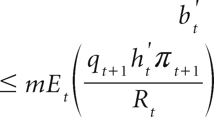
\begin{matrix} b_{t}^{'} \\ \leq m E_{t} (\frac{q_{t + 1} h_{t}^{'} π_{t + 1}}{R_{t}}) \end{matrix}

(7)

Where m denotes the LTV ratio.

Equation (7) indicates that impatient households can only borrow the maximum loan $({b^{'}}_{t})$ , which is up to the LTV ratio (m) times the expected present value of their homes.

2.2 Firms

On the production side, wholesale firms produce consumption goods, Y_t, in the consumption goods sector by using labour and capital and hiring intermediate goods from households. Also, new houses, IH_t, are produced by hiring intermediate inputs and land as well as production factor such as labor and capital in the housing sector. They try to solve the following:

\max \frac{Y_{t}}{X_{t}} + q_{t} I H_{t} - (\sum_{i = c, h} w_{i, t} n_{i, t} + \sum_{i = c, h} {w^{'}}_{i, t} {n^{'}}_{i, t} + \sum_{i = c, h} R_{i, t} z_{i, t} k_{i, t - 1} + R_{I, t} l_{t - 1} + p_{b, t} k_{b, t})

(8)

The production technologies for goods and new houses are given by:

Y_{t} = {(A_{c, t} {(n_{c, t})}^{α} {(n_{c, t}^{'})}^{1 - α})}^{1 - μ_{c}} {(z_{c, t} k_{c, t - 1})}^{μ_{c}}

(9)

I H_{t} = {(A_{h, t} {(n_{h, t})}^{α} {(n_{h, t}^{'})}^{1 - α})}^{1 - μ_{h} - μ_{b} - μ_{t}} {(z_{h, t} k_{h, t - 1})}^{μ_{h}} k_{b, t}^{μ_{b}} l_{t - 1}^{μ_{l}}

(10)

Here, A_ct and A_ht indicate productivity in the consumer goods (non-housing) sector and housing sectors, respectively; α shows patient households’ labour income share; and µ_c, µ_h, µ_b, and µ_l denote production function parameters.

2.3 Nominal Frictions

In the model, the consumption sector exhibits price rigidity, while nominal wage rigidities are allowed for both in the consumption and housing sectors. Rigidities stem from labour unions and retailers, which affect the determination of wages and prices depending on market power. Employing the Calvo (1983) pricing mechanism, retailers sell differentiated goods to households by charging a markup, X_t. The Calvo (1983) pricing style enables 1 – θ_π retailers to set prices, while the remaining θ_π retailers cannot set prices in each period; hence, they have to index prices with an elasticity of ι_π, based on the past period inflation rate.

\ln π_{t} - ι_{π} \ln π_{t - 1} = β G_{C} (E_{t} \ln π_{t + 1} - ι_{π} \ln π_{t}) - \frac{(1 - θ_{π}) (1 - β G_{C} θ_{π})}{θ_{π} \prod_{π}} \ln (\frac{X_{t}}{X}) + u_{p, t}

(11)

X denotes the steady-state price markup; the cost shock with 0 mean and variance $σ_{p}^{2}$ is presented by u_p,t. Wage-setting processes are also announced by labour unions similar to the above equation.

2.4 Monetary Policy

It is presumed that monetary policy follows the Taylor rule, which takes into account inflation and GDP growth, with interest rate smoothing to determine the nominal interest rate.

R_{t} = r_{R} R_{t - 1} + (1 - r_{R}) [r_{π} π_{t} + r_{Y} (G D P_{t} - G D P_{t - 1}) + \overset{─}{r r}] + u_{R, t} - s_{t}

(12)

where $G D P_{t} = C_{t} + I K_{t} + \bar{q} I H_{t}$ ; IK_t and IH_t show business and housing investment; and $\bar{q}$ and $\overset{─}{r r}$ denote the steady-state house price and the steady-state real interest rate, respectively. u_R,t denotes an i.i.d. monetary policy shock; and s_t denotes a shock to the inflation target and is represented by the following equation:

\ln s_{t} = ρ_{s} \ln s_{t - 1} + u_{s, t}, Ô ø Ω Ô ø Ω u_{s, t} N (0, σ_{s})

(13)

where ρ_s > 0.

2.5 Equilibrium

The cleaning conditions for consumption, housing and loan markets are as follows:

C_{t} + \frac{I K_{c, t}}{A_{k, t}} + I K_{h, t} + k_{b, t} = Y_{t} - φ_{t}

(14)

H_{t} - (1 - δ_{h}) H_{t - 1} = I H_{t}

(15)

b_{t} + b_{t}^{'} = 0

(16)

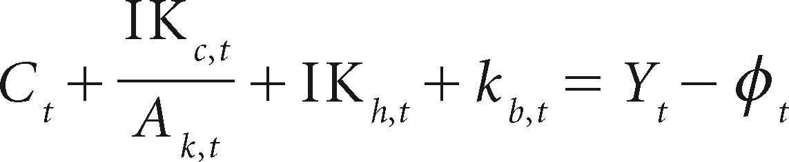
where $C_{t} = c_{t} + {c^{'}}_{t}$ shows aggregate consumption, $H_{t} = h_{t} + {h^{'}}_{t}$ shows the aggregate stock of housing and IK_c,t = k_c,t – (1 – δ_kc)k_c,t_–1 and IK_h,t = k_h,t – (1 – δ_kh)k_h,t–₁ are two components of business investment.

3. Parameter Estimation

3.1 Data

The model parameters are defined by calibration and Bayesian estimation techniques (see An & Schorfheide, 2007; Smets & Wouters, 2007; and for details of the estimation process). The model is estimated by employing Turkish quarterly data for 10 macroeconomic variables⁴ from 2010Q1 to 2019Q4. The variables are per capita real consumption, per capita real residential investment, per capita real business fixed investment, real house prices, the nominal interest rate, inflation, real wages and hours in the non-housing sector and in the housing sector. We have to begin our sample period in 2010Q1 since this is the first official house price index from CBRT. Our data are drawn from the TURKSTAT, CBRT and TRLIBOR database. We use the Census X12 procedure to de-seasonalise all the variables. Data are detrended by using the Hodrick–Prescott (HP) filter.⁵

3.2 Calibration

Table 1 lists the calibrated parameters. Some of these rely mainly on Iacoviello and Neri (2010) and Hloušek (2016) and other studies on the Turkish economy (Alp & Elekdağ, 2011; Bari & Şıklar, 2016; Çebi, 2012; Doğruel & Polat, 2015; Sekmen & Şıklar, 2016; Yüksel, 2013). The subjective discount rate for patient households (β) is set to 0.9950, which shows that the average annual real interest rate over the sample is at a steady state. We set (β'), at 0.97, which is the standard value in the DSGE literature (see Iacoviello & Neri 2010; Lee & Song 2015). The discount factor for impatient households, β', is set considerably below β, as the collateral constraint is constantly binding. In line with many studies on Turkey (Alp & Elekdağ, 2011; Doğruel & Polat, 2015; Yüksel, 2013), the markup on price and wages are set at X = X_wc = X_wh = 1.15, which implies a 15 per cent markup in the steady state. The weight on housing in the utility function is set at j = 0.12. The housing stock depreciation rate, δ_h, is chosen to be 0.0125, which reveals a 5 per cent annual depreciation of capital in the housing sector.

We also set the depreciation rates of capital δ_kc = 0.025 and δ_kh = 0.03 for the production and housing sector, respectively. We set µ_c = 0.40 for the capital share in the consumption goods production function parameter. Following Iacoviello and Neri (2010), we set µ_h = µ_b = µ_l = 0.1. One of the calibrated parameters which is important in terms of investigating the impact of monetary policy shocks on the housing market is the LTV ratio (m). We set m = 0.775, which is its average value in Turkey during the period examined. Finally, the correlation persistence of the inflation objective shock, p_s, is set at 0.975.

Table 1.
Calibrated Parameters

Parameters Definition Values

β Discount factor (for patient HHs) 0.9950

β' Discount factor (for impatient HHs) 0.97

j Housing’s weight in utility 0.12

µ_c Capital share: consumption sector 0.40

µ_h Capital share: housing sector 0.10

µ_l Land share: housing sector 0.10

µ_b Intermediate goods share: the housing sector 0.10

δ_h Depreciation rate of housing 0.0125

δ_kc Depreciation rate of capital (consumption sector) 0.025

δ_kh Depreciation rate of capital (housing sector) 0.03

X, X_wc, X_wh Mark-up prices 1.15

m Loan-to-value ratio 0.775

ρ_s Persistence of inflation objective shock 0.975

Parameters	Definition	Values
β	Discount factor (for patient HHs)	0.9950
β'	Discount factor (for impatient HHs)	0.97
j	Housing’s weight in utility	0.12
µ_c	Capital share: consumption sector	0.40
µ_h	Capital share: housing sector	0.10
µ_l	Land share: housing sector	0.10
µ_b	Intermediate goods share: the housing sector	0.10
δ_h	Depreciation rate of housing	0.0125
δ_kc	Depreciation rate of capital (consumption sector)	0.025
δ_kh	Depreciation rate of capital (housing sector)	0.03
X, X_wc, X_wh	Mark-up prices	1.15
m	Loan-to-value ratio	0.775
ρ_s	Persistence of inflation objective shock	0.975

Source: The authors.

3.3 Priors

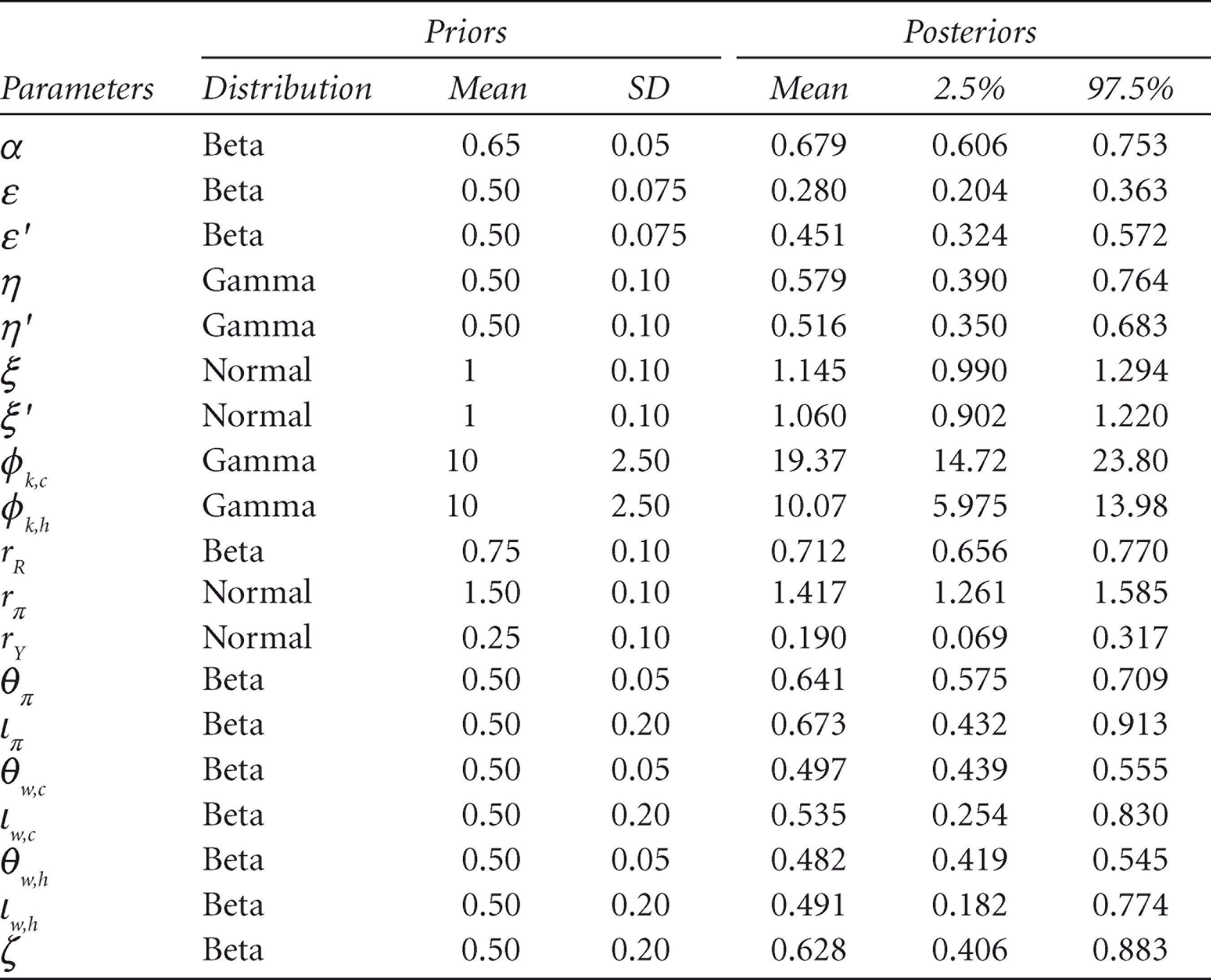
Table 2 reports the mean and distribution of the prior and posterior for all estimated parameters. For most priors, we follow similar studies (Doğruel & Polat, 2015; Hloušek, 2016; Iacoviello & Neri, 2010; Ng, 2015). The prior distribution of patient households’ income share parameter α is set at 0.65 with a standard deviation of 0.05, following a beta distribution. The prior mean for the habit parameters in consumption ε and ε' is set at 0.50, which is the same as Iacoviello and Neri (2010), Hloušek (2016) and Doğruel and Polat (2015). We impose the prior to the disutility of working η, which is set to 0.5 with a standard deviation of 0.1, in line with Iacoviello and Neri (2010). We assume an inverse elasticity of substitution across hours in the two sectors, following a normal distribution with a mean of 1 and a standard deviation of 0.1. We choose a gamma prior on the capital adjustment cost ϕ with a mean of 10 and standard deviation of 2.5. For the prior mean of the Taylor rule parameters, we impose restrictions on r_R, r_π, r_y of 0.75, 1.5 and 0.25 with a standard deviation of 0.1, respectively. The prior distribution of the Calvo price and wage parameters θ_π, θ_w,c, θ_w,h is beta with a mean of 0.5 and a standard deviation of 0.05. We assume a beta prior to the indexation parameters ι_π, ι_w,c, ι_w,h with a mean of 0.5 and a standard deviation of 0.2.

3.4 Posterior

The estimated posterior distributions of the structural parameters are shown in the right part of Table 2. It indicates that the priors are compatible with the data when considering the posterior means. Moreover, the posteriors indicate that most of the estimated parameters are similar to those in previous studies (e.g., Doğruel & Polat 2015; Hloušek, 2016; Walentin, 2014). The share of labour income for a patient household (α) is estimated to be 67.9 per cent, which also implies that the labour income for an impatient household is around 32 per cent. The values for habit formation in consumption, ε, show moderate degrees (0.28 and 0.45) in both patient and impatient households, respectively. Labour supply elasticity (η) is estimated to be 0.57 for patients and 0.51 for impatient households. The parameters ξ and ξ' are found to be 1.14 and 1.06, respectively, which implies that imperfect substitution occurs among hours in the two sectors. The adjustment cost parameters (ϕ_k,c, ϕ_k,h ) are estimated to be 19.3 and 10.1, respectively. The Taylor rule parameters are estimated as r_R = 0.71, r_π = 1.41 and r_Y = 0.19 and are slightly different from previous studies on Turkey. The estimated values of the Calvo price and wage parameter indicate that prices in Turkey are reoptimised around twice a year on average (θ_π = 0.64) and that the housing sector stickiness (θ_w,h = 0.48) is larger than that in the consumption sector (θ_w,c = 0.49).

Table 2.
Estimated Parameters

Parameters Priors
Posteriors

Distribution Mean SD Mean 2.5% 97.5%

α Beta 0.65 0.05 0.679 0.606 0.753

ε Beta 0.50 0.075 0.280 0.204 0.363

ε' Beta 0.50 0.075 0.451 0.324 0.572

η Gamma 0.50 0.10 0.579 0.390 0.764

η' Gamma 0.50 0.10 0.516 0.350 0.683

ξ Normal 1 0.10 1.145 0.990 1.294

ξ' Normal 1 0.10 1.060 0.902 1.220

ϕ_k,c Gamma 10 2.50 19.37 14.72 23.80

ϕ_k,h Gamma 10 2.50 10.07 5.975 13.98

r_R Beta 0.75 0.10 0.712 0.656 0.770

r_π Normal 1.50 0.10 1.417 1.261 1.585

r_Y Normal 0.25 0.10 0.190 0.069 0.317

θ_π Beta 0.50 0.05 0.641 0.575 0.709

ι_π Beta 0.50 0.20 0.673 0.432 0.913

θ_w,c Beta 0.50 0.05 0.497 0.439 0.555

ι_w,c Beta 0.50 0.20 0.535 0.254 0.830

θ_w,h Beta 0.50 0.05 0.482 0.419 0.545

ι_w,h Beta 0.50 0.20 0.491 0.182 0.774

ζ Beta 0.50 0.20 0.628 0.406 0.883

Parameters	Priors	Posteriors
α	Beta	0.65	0.05	0.679	0.606	0.753
ε	Beta	0.50	0.075	0.280	0.204	0.363
ε'	Beta	0.50	0.075	0.451	0.324	0.572
η	Gamma	0.50	0.10	0.579	0.390	0.764
η'	Gamma	0.50	0.10	0.516	0.350	0.683
ξ	Normal	1	0.10	1.145	0.990	1.294
ξ'	Normal	1	0.10	1.060	0.902	1.220
ϕ_k,c	Gamma	10	2.50	19.37	14.72	23.80
ϕ_k,h	Gamma	10	2.50	10.07	5.975	13.98
r_R	Beta	0.75	0.10	0.712	0.656	0.770
r_π	Normal	1.50	0.10	1.417	1.261	1.585
r_Y	Normal	0.25	0.10	0.190	0.069	0.317
θ_π	Beta	0.50	0.05	0.641	0.575	0.709
ι_π	Beta	0.50	0.20	0.673	0.432	0.913
θ_w,c	Beta	0.50	0.05	0.497	0.439	0.555
ι_w,c	Beta	0.50	0.20	0.535	0.254	0.830
θ_w,h	Beta	0.50	0.05	0.482	0.419	0.545
ι_w,h	Beta	0.50	0.20	0.491	0.182	0.774
ζ	Beta	0.50	0.20	0.628	0.406	0.883

Source: The authors.

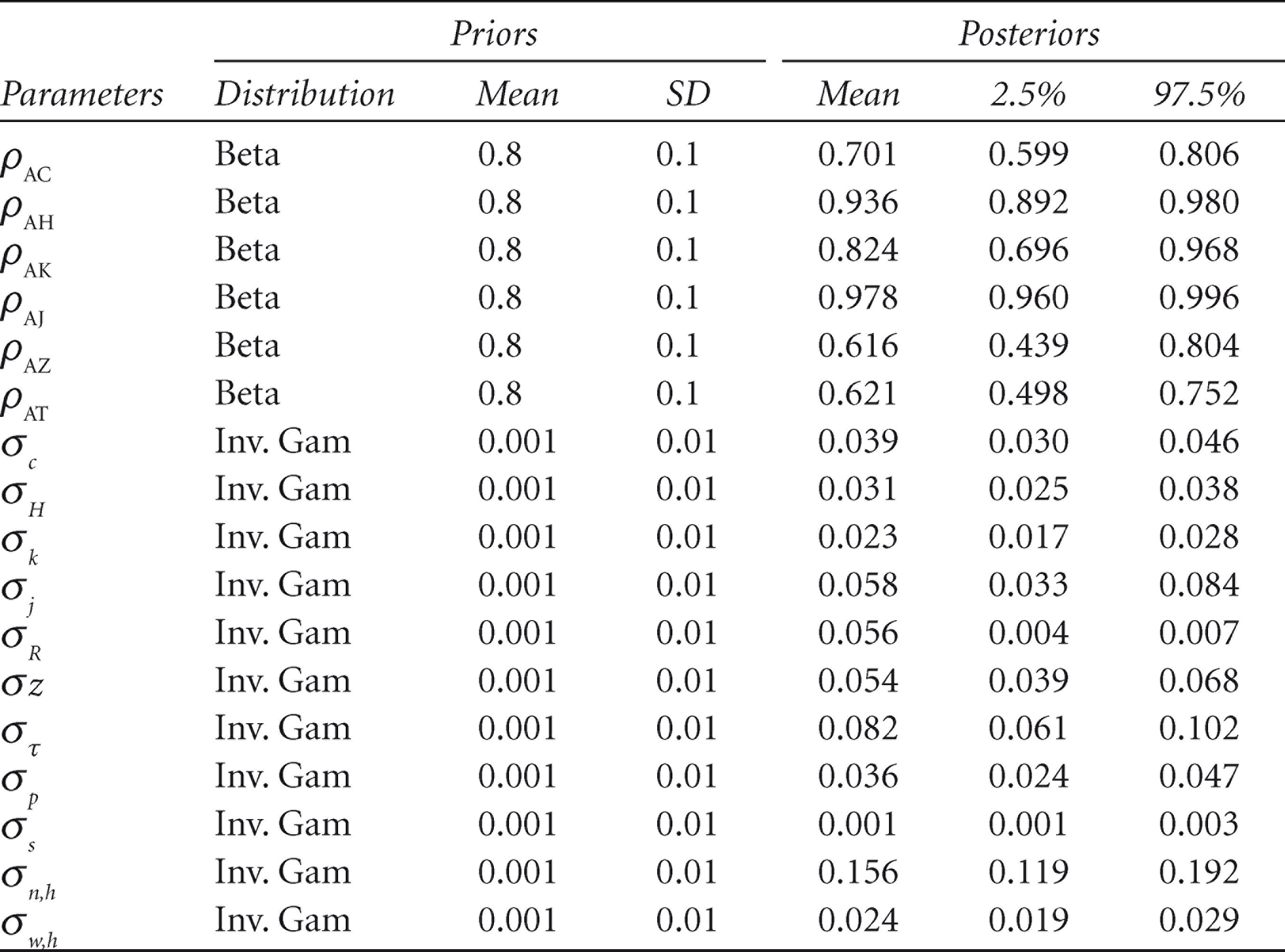
The priors and posteriors for the shock process are presented in Table 3. We impose an inverse gamma prior to the standard deviation of each shock, with a mean of 0.001 and a standard deviation of 0.1. We set a beta distribution with a prior mean of 0.8 and a standard deviation of 0.1 for the AR (autoregressive) coefficients. It shows that the stochastic process for exogenous innovation is quite persistent. The shock coefficients vary between 0.61 and 0.97. The housing preference (ρ_AJ) and housing technology (ρ_AH) shocks are estimated to be highly persistent, at 0.97 and 0.93, respectively. These findings are similar to those in Iacoviello and Neri (2010), Walentin (2014) and Hloušek (2016). Monetary policy (ρ_AC) and business investment (ρ_AK) shocks are moderately persistent, with AR (1) coefficients of 0.70 and 0.82, respectively.

Table 3.

Shock Parameter Estimations

Parameters	Priors			Posteriors
Parameters	Distribution	Mean	SD	Mean	2.5%	97.5%
ρ _AC	Beta	0.8	0.1	0.701	0.599	0.806
ρ _AH	Beta	0.8	0.1	0.936	0.892	0.980
ρ _AK	Beta	0.8	0.1	0.824	0.696	0.968
ρ _AJ	Beta	0.8	0.1	0.978	0.960	0.996
ρ _AZ	Beta	0.8	0.1	0.616	0.439	0.804
ρ _AT	Beta	0.8	0.1	0.621	0.498	0.752
σ_c	Inv. Gam	0.001	0.01	0.039	0.030	0.046
σ_H	Inv. Gam	0.001	0.01	0.031	0.025	0.038
σ_k	Inv. Gam	0.001	0.01	0.023	0.017	0.028
σ_j	Inv. Gam	0.001	0.01	0.058	0.033	0.084
σ_R	Inv. Gam	0.001	0.01	0.056	0.004	0.007
σz	Inv. Gam	0.001	0.01	0.054	0.039	0.068
σ_τ	Inv. Gam	0.001	0.01	0.082	0.061	0.102
σ_p	Inv. Gam	0.001	0.01	0.036	0.024	0.047
σ_s	Inv. Gam	0.001	0.01	0.001	0.001	0.003
σ_n,h	Inv. Gam	0.001	0.01	0.156	0.119	0.192
σ_w,h	Inv. Gam	0.001	0.01	0.024	0.019	0.029

Source: The authors.

4. Quantitative Results

In this part of the article, the quantitative results obtained from the model are considered to evaluate housing market dynamics in Turkey. First, the effects of monetary policy and housing market-related shocks on the variables in the model are explained by using impulse response analysis. Secondly, variance decompositions reveal the contribution of each shock in our model to the variance of the consumption, residential investment, business investment, house prices, inflation, interest rate and GDP. Finally, the historical decomposition of variables such as real house prices, residential investment and GDP indicate the relative importance of each shock for fluctuations in the variables over all periods examined.

4.1 Impulse Response Analysis

The behaviour of the model in response to shocks is investigated under different LTV values. There are three different specifications to observe the effect of macroprudential policies on the housing market. In the first, the LTV ratio is set to 0.775, which is called the benchmark specification. Secondly, the LTV ratio is set to 0.95, the high collateral specification, which allows impatient households more borrowing opportunities. Finally, to observe the implications on impatient households which are not allowed to access the financial market, LTV is set to 0 in the no collateral specification. In the analysis of macroprudential policies, a high LTV value of the housing market is generally considered procyclical and a tool that increases consumption and thus enhances output (Bouda & Formanek, 2014).

We conduct the impulse responses analysis under three different shocks, which are housing preference, housing technology and monetary policy shocks, to observe the behaviour of real consumption, residential investment, business investment, house prices, inflation, interest rate and output. All the values are expressed as the percentage deviation from the steady-state value. Note that a period in the impulse response graphs represents a quarterly period.

Housing Preference Shock

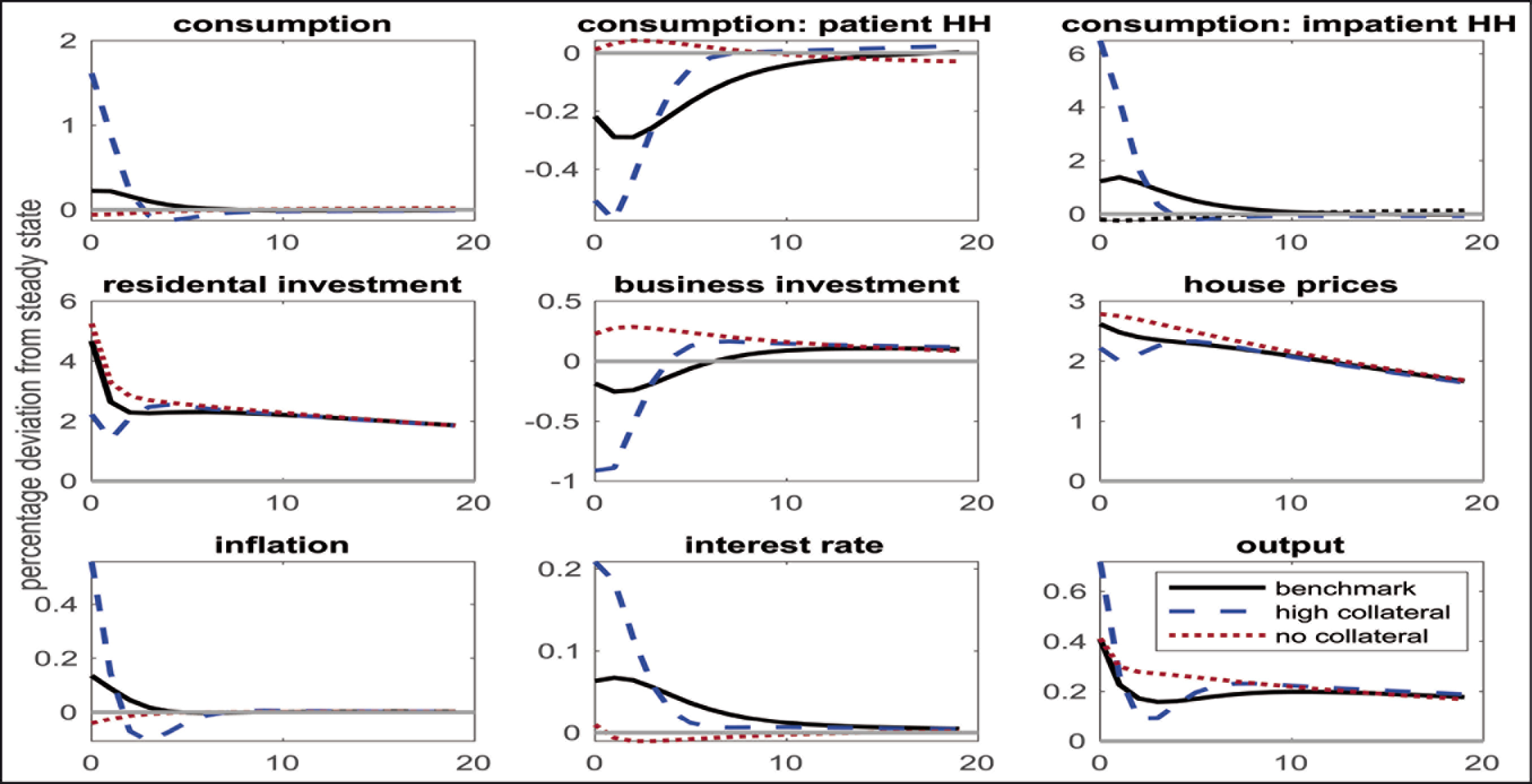
Figure 2 shows the impacts of a housing preference⁶ (housing demand) shock on macroeconomic variables. As a result of the increase in housing demand, house prices go up. In all three specifications, housing demand shocks have a positive effect on house prices. This shock enhances the possibility of borrowing by households who want to use their houses as collateral, thus facilitating their borrowing and consumption under the high collateral scenario. Since consumption by impatient households is higher, this has a positive effect on total consumption, even if patient consumption contracts (Lee & Song, 2015). Also, while residential investment increases after a housing preference shock, business investment declines in the no collateral and high collateral specifications, since resources in the economy shift from business investment to housing investment in the short term. The increase in consumption and housing investment leads to an increase in economic output.

An increase in the value of the collateral as a result of the surge in housing prices triggers the consumption of impatient households (as in Doğruel & Polat, 2015; Iacoviello & Neri, 2010; Walentin, 2014) and creates an inflationary pressure in the economy,⁷ causing the monetary authority to increase the interest rate. However, Figure 2 shows that the increase in the interest rate in the high collateral scenario is higher than in the other scenarios. As a result, the negative effect of the high interest rate on output is greater in the high collateral scenario. Consequently, housing demand shocks in the model create a procyclicality movement among the examined variables, owing to the collateral effect that strengthens the relationship between housing prices and consumption.

Figure 2.

Source: The authors.

Monetary Policy Shock

Figure 3 shows the responses to positive monetary policy shocks, which increase the nominal interest rate under the three scenarios. It indicates that the patterns of the impulse responses are very similar and a decline in all items of output (i.e., consumption and residential and business investment) and in house prices. The decrease in house prices following a contractionary monetary policy shock is in line with most of the empirical housing literature (Assenmacher-Wesche & Gerlach, 2008; Bjørnland & Jacobsen, 2010; Elbourne, 2008). Under the high collateral and benchmark scenarios, the consumption of patient households rises temporarily, but the consumption of impatient households decreases for all three scenarios, since the drop in house prices brings down their borrowing capacity. Another outcome of the monetary policy shock is that an increase in the interest rate causes the inflation rate to decrease by 0.5 per cent. This finding can be interpreted as indicative of the efficiency of monetary policy in controlling inflation.

Figure 3.

Source: The authors.

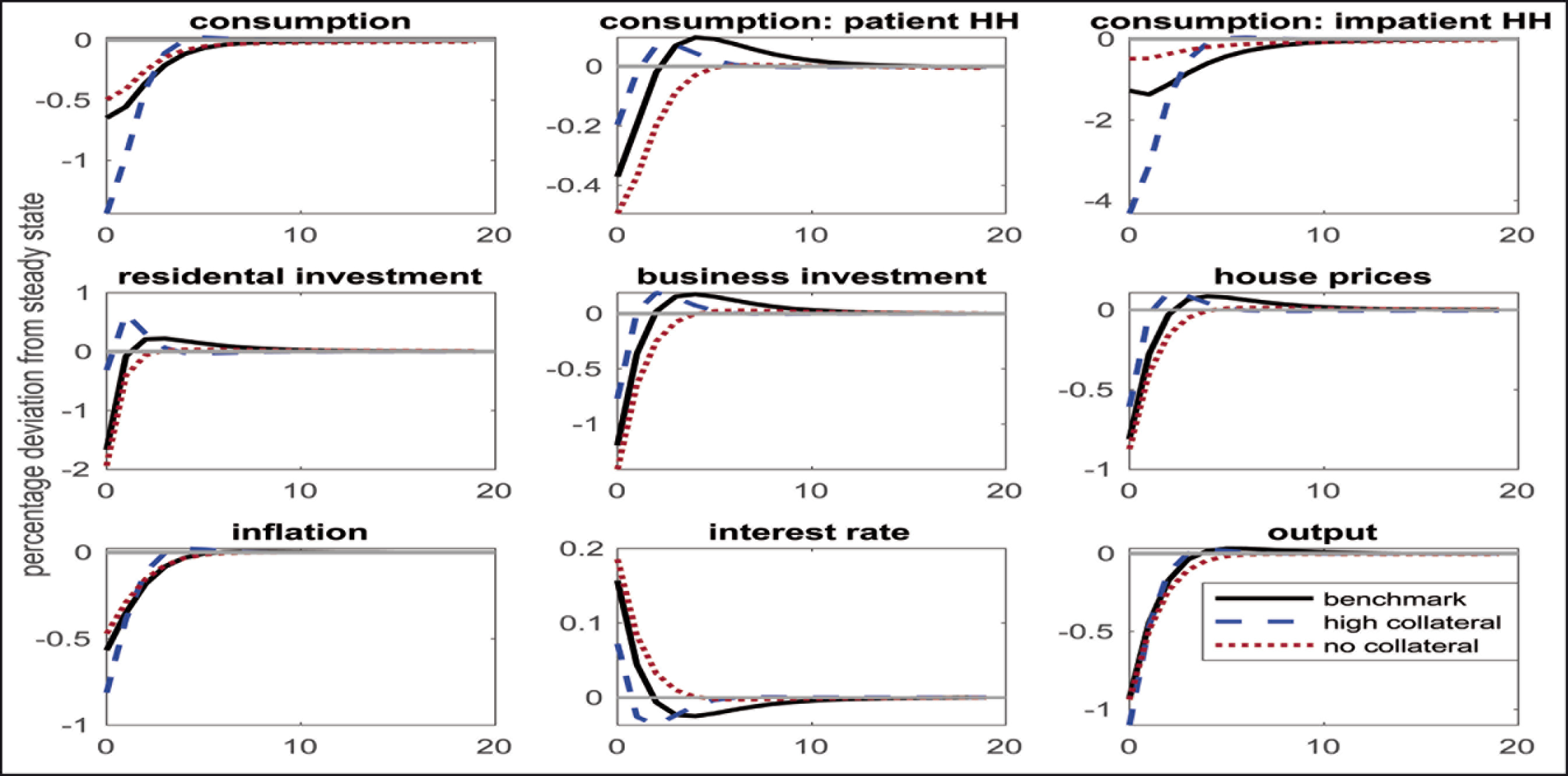
Moreover, an increase in the interest rate in Turkey leads to a reduction in consumption and investment, and therefore in economic output, which is consistent with the conventional monetary transmission mechanism in economics. The effect of monetary policy shocks in the three scenarios reveals striking results. After an increase in m from 0.775 to 0.95, the relative decline in inflation is less than the decrease in consumption and economic output. This reveals two outcomes. First, that monetary policy shocks work through the collateral channel when the effect of high LTVs is considered, and the effects of the shocks are further strengthened. Second, the response of real variables, such as consumption and output, is higher than the response of inflation. Based on these findings, it can be said that a contractionary (tight) monetary policy aimed at lowering inflation may lead to relatively larger decreases in real variables such as consumption and investment compared to inflation when the LTV ratio is high. The response of residential investment to monetary policy is negative. Wage rigidities in the housing sector play an important role in explaining this, as it makes housing investment very responsive to monetary policy shocks. As a result of higher interest rates (contractionary monetary policy), housing demand and house prices go down while wages in the housing sector remain constant. This leads to a fall in housing investment because of decreasing profitability.

Housing Technology Shock

Figure 4 shows the responses of nine variables to a housing technology shock. Since this shock relates to the marginal efficiency of producing housing, it is called as a housing-specific technology shock. Note that a positive shock to housing-specific technology will reduce the price of building houses. This shock in the housing sector leads to a considerable rise in residential investment. Since it represents housing supply, house prices fall due to technological progress over a long-term horizon. The consumption of impatient households, which enable the possibility of borrowing through the value of their housing, decreases as a result of a decrease in house prices. However, the decline in the consumption of impatient households has been the main driver of the decline in consumption even though consumption of patient households has slightly increased in the high collateral scenario. As expected, the nominal interest rate goes down and the inflation rate also falls in response to housing technology shocks. These findings are in line with those of Iacoviello and Neri (2010), Walentin (2014), Hloušek (2016) and Doğruel and Polat (2015).

Figure 4.

Source: The authors.

The impact of the technology shock in the housing sector on consumption shows that the collateral channel works effectively. While the technology shock decreases house prices and borrowing opportunities for impatient households, at the same time, it decreases inflation. For this, the response of the collateral effect on inflation and house prices is in the same direction; monetary policy, housing preference and housing technology shock are significant. Since the permanence parameter of the housing technology shock has a very high AR (1) autoregressive process, 0.93, it is observed that the effect of the shock is long.

4.2 Variance Decomposition

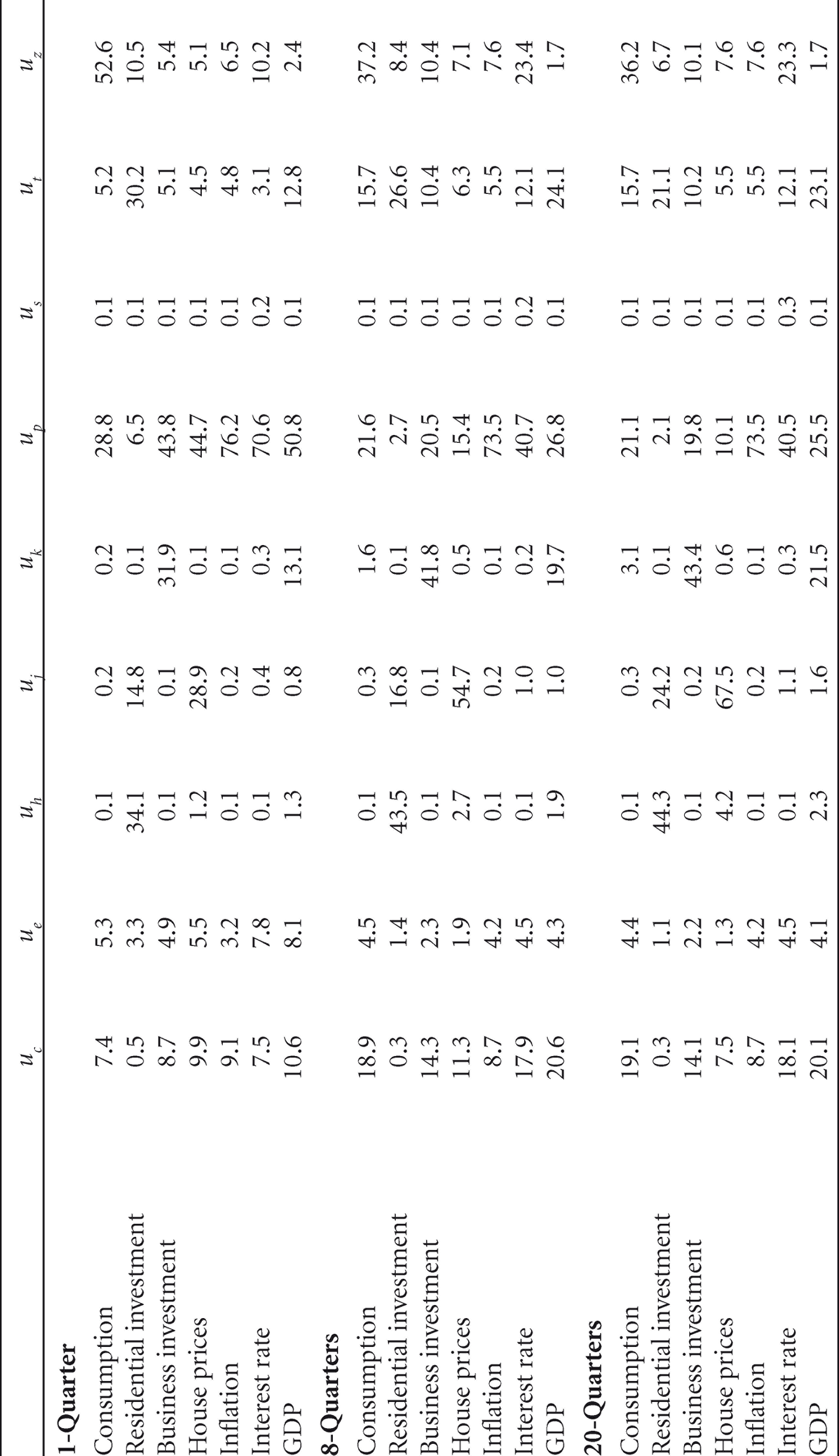
The findings from variance decompositions are shown in Table 4, which indicates how much of the forecast error variance of each variable can be explained by exogenous shocks to other variables. There are nine exogenous shocks to the model economy: u_c —consumption goods shocks; u_e —monetary policy shocks; u_h —housing technology shocks; u_j —housing preference shocks; u_k —business investment shocks; u_z — intertemporal preference shocks; u_π—labour supply shocks; u_p—cost-push shocks; and u_s—inflation-targeting shocks.

Table 4.
Conditional Variance Decomposition

u_c u_e u_h u_j u_k u_p u_s u_t u_z

1-Quarter

Consumption 7.4 5.3 0.1 0.2 0.2 28.8 0.1 5.2 52.6

Residential investment 0.5 3.3 34.1 14.8 0.1 6.5 0.1 30.2 10.5

Business investment 8.7 4.9 0.1 0.1 31.9 43.8 0.1 5.1 5.4

House prices 9.9 5.5 1.2 28.9 0.1 44.7 0.1 4.5 5.1

Inflation 9.1 3.2 0.1 0.2 0.1 76.2 0.1 4.8 6.5

Interest rate 7.5 7.8 0.1 0.4 0.3 70.6 0.2 3.1 10.2

GDP 10.6 8.1 1.3 0.8 13.1 50.8 0.1 12.8 2.4

8-Quarters

Consumption 18.9 4.5 0.1 0.3 1.6 21.6 0.1 15.7 37.2

Residential investment 0.3 1.4 43.5 16.8 0.1 2.7 0.1 26.6 8.4

Business investment 14.3 2.3 0.1 0.1 41.8 20.5 0.1 10.4 10.4

House prices 11.3 1.9 2.7 54.7 0.5 15.4 0.1 6.3 7.1

Inflation 8.7 4.2 0.1 0.2 0.1 73.5 0.1 5.5 7.6

Interest rate 17.9 4.5 0.1 1.0 0.2 40.7 0.2 12.1 23.4

GDP 20.6 4.3 1.9 1.0 19.7 26.8 0.1 24.1 1.7

20-Quarters

Consumption 19.1 4.4 0.1 0.3 3.1 21.1 0.1 15.7 36.2

Residential investment 0.3 1.1 44.3 24.2 0.1 2.1 0.1 21.1 6.7

Business investment 14.1 2.2 0.1 0.2 43.4 19.8 0.1 10.2 10.1

House prices 7.5 1.3 4.2 67.5 0.6 10.1 0.1 5.5 7.6

Inflation 8.7 4.2 0.1 0.2 0.1 73.5 0.1 5.5 7.6

Interest rate 18.1 4.5 0.1 1.1 0.3 40.5 0.3 12.1 23.3

GDP 20.1 4.1 2.3 1.6 21.5 25.5 0.1 23.1 1.7

	u_c	u_e	u_h	u_j	u_k	u_p	u_s	u_t	u_z
1-Quarter
Consumption	7.4	5.3	0.1	0.2	0.2	28.8	0.1	5.2	52.6
Residential investment	0.5	3.3	34.1	14.8	0.1	6.5	0.1	30.2	10.5
Business investment	8.7	4.9	0.1	0.1	31.9	43.8	0.1	5.1	5.4
House prices	9.9	5.5	1.2	28.9	0.1	44.7	0.1	4.5	5.1
Inflation	9.1	3.2	0.1	0.2	0.1	76.2	0.1	4.8	6.5
Interest rate	7.5	7.8	0.1	0.4	0.3	70.6	0.2	3.1	10.2
GDP	10.6	8.1	1.3	0.8	13.1	50.8	0.1	12.8	2.4
8-Quarters
Consumption	18.9	4.5	0.1	0.3	1.6	21.6	0.1	15.7	37.2
Residential investment	0.3	1.4	43.5	16.8	0.1	2.7	0.1	26.6	8.4
Business investment	14.3	2.3	0.1	0.1	41.8	20.5	0.1	10.4	10.4
House prices	11.3	1.9	2.7	54.7	0.5	15.4	0.1	6.3	7.1
Inflation	8.7	4.2	0.1	0.2	0.1	73.5	0.1	5.5	7.6
Interest rate	17.9	4.5	0.1	1.0	0.2	40.7	0.2	12.1	23.4
GDP	20.6	4.3	1.9	1.0	19.7	26.8	0.1	24.1	1.7
20-Quarters
Consumption	19.1	4.4	0.1	0.3	3.1	21.1	0.1	15.7	36.2
Residential investment	0.3	1.1	44.3	24.2	0.1	2.1	0.1	21.1	6.7
Business investment	14.1	2.2	0.1	0.2	43.4	19.8	0.1	10.2	10.1
House prices	7.5	1.3	4.2	67.5	0.6	10.1	0.1	5.5	7.6
Inflation	8.7	4.2	0.1	0.2	0.1	73.5	0.1	5.5	7.6
Interest rate	18.1	4.5	0.1	1.1	0.3	40.5	0.3	12.1	23.3
GDP	20.1	4.1	2.3	1.6	21.5	25.5	0.1	23.1	1.7

Source: The authors.

In all periods, housing technology, housing preferences and labour supply shocks largely account for residential investment fluctuations. In the long term (20-quarter horizon), housing-related shocks explain 68.5 per cent of the variation in residential investment. In the very short term (1-quarter horizon), movements in house prices are largely explained by housing preference shocks (28.9%) and cost-push shocks (44.7%). The shock on consumption goods does not have any effect on the movement in house prices: in the very short term, it explains 9.9 per cent of the movement in house prices, while in the long term, it accounts for 7.5 per cent of variations in house prices. In the medium term (8-quarter horizon) and long term, the main contributors to house price fluctuations stem from house preference shocks, which accounts for 54.7 per cent of house price fluctuations for 8-quarters and 67.5 per cent for 20-quarters. These results indicate that the demand for housing is the predominant driving force of fluctuations in house prices in Turkey.⁸ It is seen that consumption good shocks and cost shocks affect not only nominal variables, but also real variables (i.e., the GDP) in the very short term. However, the impact of the cost shock on GDP decreases in the medium term and long term, while the impact of the consumption goods shocks increases, especially on GDP.

Another result is that the effect of a monetary policy shock on movements in house prices is limited, compared to a housing demand shock. This shows that the variation on consumption is determined by intertemporal preference shocks (36.2%), cost-push shocks (21.1%) and consumption goods shocks (19.1%) over the long-term period. Fluctuations in the GDP are not well explained by housing preference shocks, but approximately 90 per cent of GDP is explained by the shocks in the consumption goods sector (20.1%), business investment (21.5%), cost-push (25.5%) and labour supply (23.1%). At the end of 20-quarters, both housing technology (2.3%) and housing preference (1.6%) shocks account for less than 4 per cent of the variance in GDP and less than 1 per cent of consumption and inflation variations, respectively. The variance decomposition results reveal that the shock from labour supply is one of the most important shocks accounting for variations in consumption, investment and GDP. This shows that Turkey’s economy, with its abundant labour force, and despite the drawbacks of technology, has for many years depended on developments in the highly labour-intensive industry structure. Therefore, a change in the supply of labour has a significant impact on the entire economy. Also, it is observed that cost-push shocks are an important driver of business cycle fluctuations in Turkey, whereas the central bank’s inflation-targeting shocks do not play any significant role.

The variance decomposition analysis (Table 5) reveals the amplification mechanism of the LTV ratio under three different collateral constraints (i.e., high, benchmark and no-collateral) on consumption, output and inflation, by considering the monetary policy shock. We can easily compare these variance decomposition results to those under the no-collateral, benchmark and high collateral scenarios. In the case of the high collateral scenario, the effect of monetary policy shocks, mainly on consumption (more than 2 times), is higher than on inflation and output. In the case where impatient households are excluded from the loan market (m = 0), fluctuations in the variables are moderately explained by monetary policy shocks. However, there is little difference in the benchmark situation. This indicates that the high collateral scenario considerably amplifies the effect of the monetary policy shock. This amplification is strongest in consumption, followed by inflation and then output, which is in line with findings for other countries (Hloušek, 2016; Walentin, 2014). Therefore, using the LTV ratio as an efficient macro prudential tool to reduce the number of adverse effects that arise from housing policy may stabilise the fluctuation of business cycles (Bruneau et al., 2018).

Table 5.

The Importance of Collateral Constraint: The Monetary Policy Shock for Variance Decomposition (%)

Scenario	Consumption	Output (GDP)	Inflation
High collateral (m = 0.95)	10.4	5.32	7.46
Benchmark (m = 0.775)	4.28	3.97	4.26
No collateral (m = 0)	2.75	4.14	2.75

Source: The authors.

Similarly, housing demand shocks have the same effect on the variables (Table 6). The analysis shows that the spillover effect from the housing sector to the other side of the economy is not insignificant, and that the determination of the LTV ratio is important for the rest of the economy. The impact of the housing preference shock is very high, particularly in terms of consumption and inflation, in the case of the high collateral scenario. With a higher positive preference shock, real house prices rise, and this leads to an increase in the collateral capacity of impatient households which in turn boosts borrowing and consumption.

Table 6.

Importance of Collateral Constraint: The Housing Preference Shock for Variance Decomposition (%)

Scenario	Consumption	Output (GDP)	Inflation
High collateral (m = 0.95)	5.91	4.85	1.85
Benchmark (m = 0.775)	0.30	2.67	0.21
No collateral (m = 0)	0.06	2.72	0.02

Source: The authors.

4.3 Historical Shock Decompositions

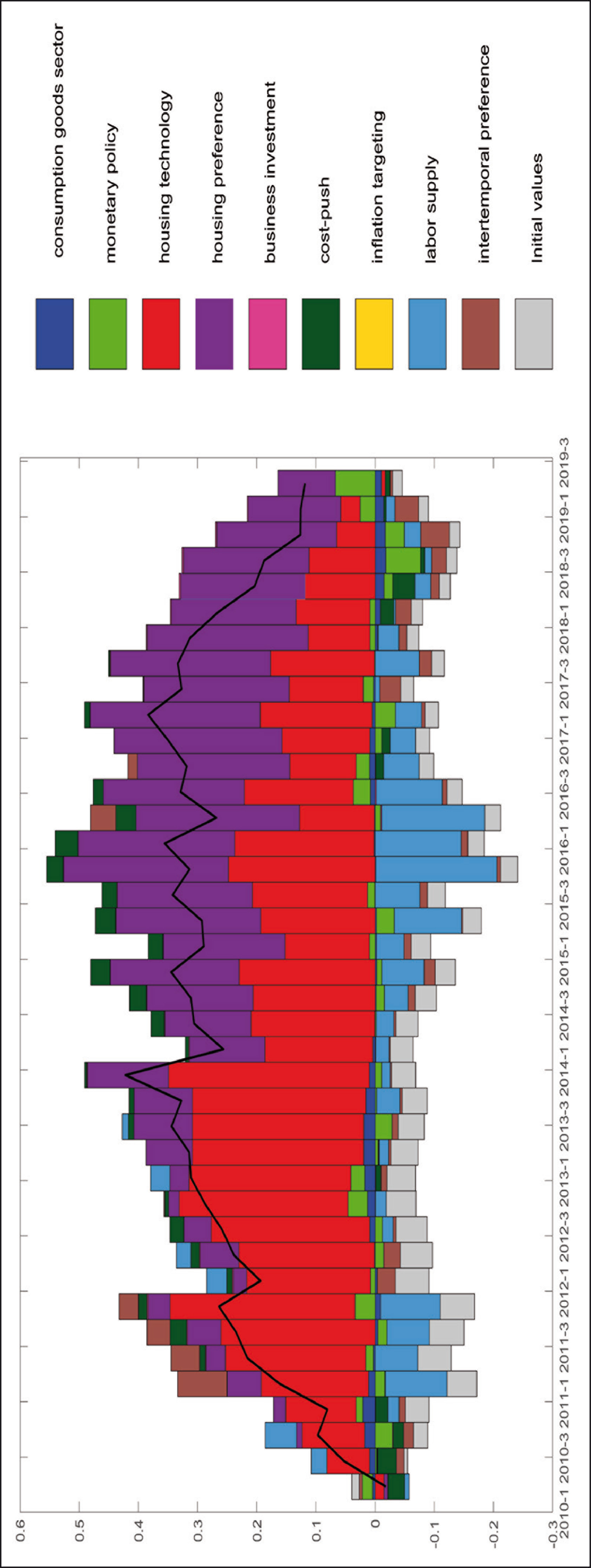
Figures 5 and 6 depict the historical shock decomposition of real house prices, residential investment and GDP according to the structural shocks in the model over the period 2010Q1 to 2019Q4. In line with the variance decomposition results, the historical shock decomposition indicates that housing preference shocks are the main drivers of real house prices in Turkey. Since 2013, housing preference shocks have contributed most to changes in house prices, followed by consumption goods sector shocks. The historical shock decomposition further suggests that the contribution of monetary policy has become more important in recent years. The results of the historical shock decomposition of housing prices are similar to those noted by Iacoviello and Neri (2010), contrary to Walentin (2014) which shows that that real housing price fluctuations are negatively affected by monetary policy shocks for Sweden. Further, Ng (2015) and Lee and Song (2015) find that housing preference shocks play a key role in house prices for China and Korea, respectively.

Figure 5.

Source: The authors.

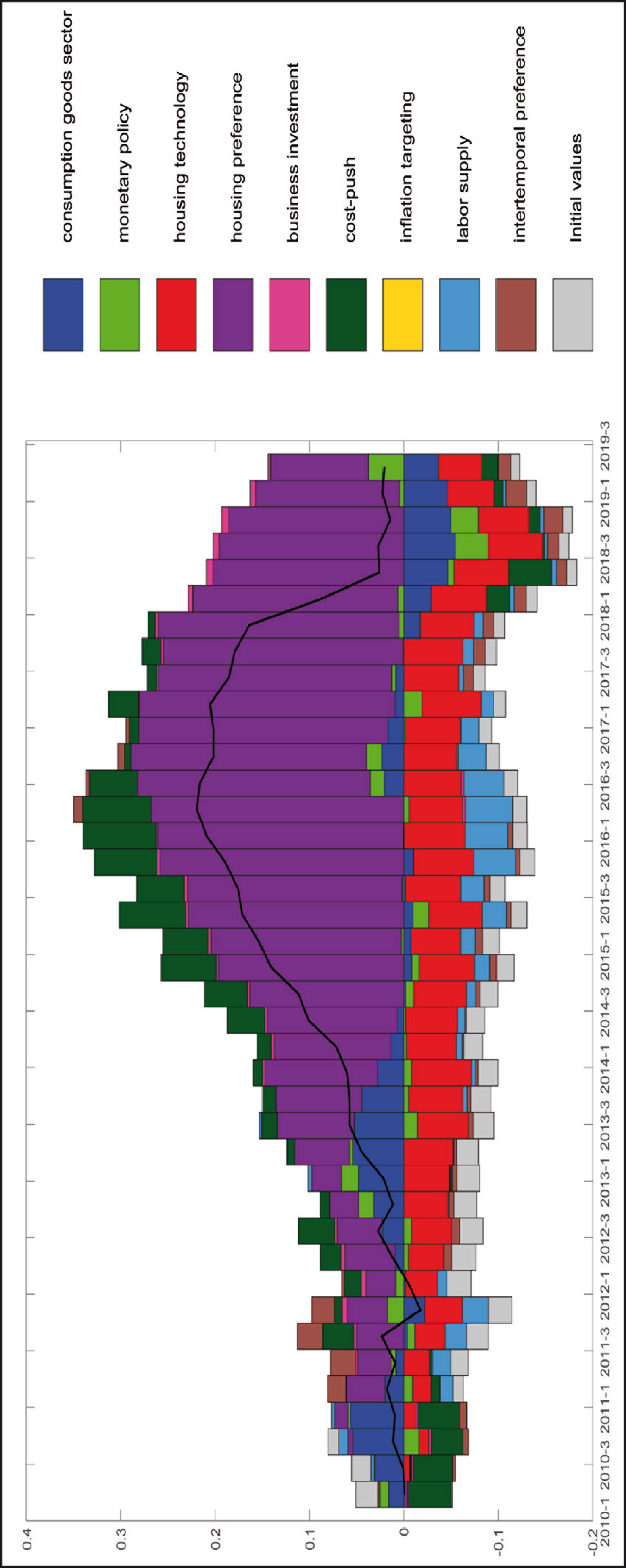
Although housing investments have generally followed an increasing trend in the period 2010–2019, there has been a rapid contraction after 2018 (Figure 6). Shocks from housing technology and housing preferences almost equally account for the fluctuations in residential investment after 2014, as indicated by the results of the variance decomposition. Housing technology shocks were almost the only determinant factor until 2013, except for weak impacts from shocks in the consumer goods sector and monetary policy. After 2013, housing preference shocks play an increasing role in explaining the variance in housing investments. Similar to our findings, Ng (2015) finds that housing preference and housing technology shocks are equally important for residential investments, as do Doğruel and Polat (2015) who suggest that housing technology shocks have a dominant effect on residential investments for the period 2010 to 2014 in Turkey.

Figure 6.

Source: The authors.

4.4 Counterfactual Analysis

In this section, we evaluate the effect of traditional monetary policy on helping to stabilise house prices. For this, we extend the Taylor rule to the case in which CBRT responds to fluctuations in house prices. In literature, there is no consensus on whether central banks should respond to housing prices or not. However, in recent years, there have been several studies that analyse the extended Taylor rule by incorporating asset and house prices in the central bank’s response function (Aspachs-Bracons & Rabanal, 2011; Finocchiaro & Heideken, 2013; Fuhrer & Tootell, 2008; Gupta & Sun, 2020; Kannan et al., 2012; Notarpietro & Siviero, 2015; Sun & Tsang, 2014). However, so far, there has been no study which takes into account house prices in Turkey.

Equation (17) is an extension of Equation (12) with house prices, which represents the standard monetary policy according to the Taylor rule; nq_t and r_q denote nominal house prices and the responsiveness of changes in house prices in the reaction function of the central bank, respectively.

R_{t} = r_{R} R_{t - 1} + (1 - r_{R}) [r_{π} π_{t} + r_{Y} (G D P_{t} - G D P_{t - 1}) + \overset{─}{r r} + r_{q} (n q_{t} - n q_{t - 1})] + u_{R, t} - s_{t}

(17)

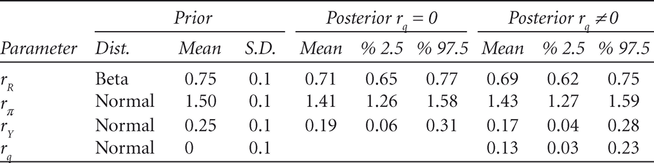
Table 7 shows the estimation results of the parameters in the extended Taylor rule, in which only the parameters of the Taylor equation are altered by keeping all other parameters in the model constant. We set 0 prior means with 0.1 standard deviations for r_q. Such an assignment is consistent to estimate the model to understand the importance of the coefficient.

Table 7 shows the mean and standard deviation of the prior and posterior distributions, both for the benchmark Taylor rule model [in which the central bank does not pay attention to house prices (r_q = 0) and the extended Taylor rule model (r_q 0) in Turkey. In the extended model where the interest rate reacts to house price inflation, the posterior mean of r_q is 0.13. It can be inferred from our main result that house price fluctuations do not play a substantial role in CBRT’s reaction function over the sample period as expected. CBRT has reacted less aggressively to increases in house prices than to inflation (1.43) and output fluctuations (0.17). The posterior means of the other Taylor rule parameters (r_R, r_π, r_Y) are similar to the benchmark Taylor rule models, which show the robustness of the two models estimated.

Table 7.

Priors and Posteriors of the Extended Taylor Rule

Parameter	Prior			Posterior r_q = 0			Posterior r_q ¹ 0
Parameter	Dist.	Mean	S.D.	Mean	% 2.5	% 97.5	Mean	% 2.5	% 97.5
r_R	Beta	0.75	0.1	0.71	0.65	0.77	0.69	0.62	0.75
r_π	Normal	1.50	0.1	1.41	1.26	1.58	1.43	1.27	1.59
r_Y	Normal	0.25	0.1	0.19	0.06	0.31	0.17	0.04	0.28
r_q	Normal	0	0.1				0.13	0.03	0.23

Source: The authors.

Unfortunately, we cannot compare our results with the other studies that consider Taylor rules with house prices in Turkey. However, the parameters for the US Fed, the Bank of England (BoE) and Bank of Japan (BoJ) are found to be 0.36, 0.16 and 0.26, respectively, in Finocchiaro and Heideken (2013). Recently, Gupta and Sun (2020) found that the house price responsiveness parameter for South Africa was 0.58. When we compare that parameter to the other important central bank’s reaction functions, we see that the CBRT’s response parameter (r_q) to house price growth is lower than that for the FED, BoJ and South African Reserve Bank. Our findings make a significant contribution to the empirical literature on estimating DSGE models for all developing countries, including Turkey. Moreover, they enable us to examine the shocks behind housing market dynamics in those countries.

Table 8 presents the unconditional variance decomposition results of the model estimated by the extended Taylor rule. When we consider the variance decomposition findings, which are very similar to the results obtained in the previous part of the study, 62.2 per cent of the fluctuations in house prices are explained by housing demand shocks. The housing preference (30.7%) and housing technology shocks (41.4%) account for about 72.1 per cent of the variations in residential investment. The variation in GDP is mostly explained by consumption goods (19.1%), labour supply (20.8%), cost-push (25.8) and business investment (23.2%) shocks.

Table 8.

Variance Decomposition of the Extended Taylor Rule

	u_c	u_e	u_h	u_j	u_k	u_p	u_s	u_t	u_z
Consumption	20.7	3.3	0.1	0.1	8.1	26.7	0.1	17.1	23.8
Residential investment	0.3	1.4	41.4	30.7	0.1	1.8	0.1	18.3	5.9
Business investment	13.8	2.5	0.1	0.5	42.1	19.2	0.1	10.4	11.4
House prices	6.7	1.3	9.8	62.2	1.9	9.1	0.1	3.9	5.1
Interest rate	17.3	6.4	0.1	2.1	0.7	38.4	0.1	12.8	22.1
GDP	19.1	3.6	2.1	2.2	23.2	25.8	0.1	20.8	3.1

Source: The authors.

5. Conclusion

House prices in Turkey have experienced a substantial increase since the early-2010s. However, after 2016, this rapid boom in house prices has slowed down with lower GDP growth in Turkey. Following the CBRT’s gradual lowering of its policy rate after 2018Q3, house prices have once more started to increase. In this article, we examine the dynamics of the housing market in Turkey by estimating a DSGE model which takes into account the collateral role of financial constraints for housing.

The findings can be summarised as follows: First, the important historical driver of house prices in Turkey since 2010 is housing demand shocks. Although monetary policy is generally not the main determinant of house prices in Turkey, its contribution has become more important in recent years. Housing market-specific shocks (e.g., housing preference and housing technology), however, have not contributed greatly to explaining real variables such as consumption and output. Variations in residential investment are mainly explained by housing technology and housing preference shocks. Secondly, our findings reveal that regulations in the LTV ratio can be treated as a valuable macroprudential tool to mitigate the economic instability caused by fluctuations in the housing market. According to the impulse response functions and variance decomposition analysis under three different LTV ratios, consumption and output display a stronger response to housing demand and monetary policy shocks under the high collateral scenario. It can be inferred that the collateral effects of housing market shocks are stronger in the highest LTV scenario.

Variance decomposition findings suggest that approximately 6 per cent of the consumption variance in the high collateral model is explained by the housing preference shock, and approximately 1 per cent in the benchmark scenario. Similarly, the monetary policy shock has a reinforcing effect on consumption and output. It increases the impact of the variances from 4.28 per cent to 10.4 per cent for consumption and from 3.97 per cent to 5.32 per cent for output. This gives us important information about appropriate macroprudential policies for household borrowing conditions that would substantially influence the relationship between the housing market and the rest of the macroeconomy. Thirdly, we investigate whether the Central Bank of Turkey has actively reacted to increases in the house prices since 2010. Our findings show that fluctuations in house prices have not played a substantial role in the monetary policy reaction function of Turkey.

Finally, from the perspective of macroeconomic policy, three important policy instruments have impacted the development of the housing market in recent years—excessive credit growth, loose monetary policy and weak regulatory policy. The rapid increase in housing loans plays a key role in soaring housing prices in Turkey. Also, the government has incentivised households to buy housing by reducing real estate taxes, which has increased housing demand and house prices in turn. However, the skyrocketing of house prices, fuelled by the increase in mortgage loans and government-led promotions, has raised concerns about the long-term stability and the economic fundamentals of house prices.

More importantly, public banks have recently started to provide housing loans at below market rates to boost the housing market, which has led to a deterioration in the efficiency of the financial market. The credit-driven growth pattern in the Turkish economy is clear from the functioning of the housing market. For these reasons, one can easily claim that macroprudential tools to prevent financial instability do not work effectively in Turkey. The rapid increase in housing loans as well as high house prices, leading to an erosion of the long-term national saving rate in Turkey’s economy, is a threat to economic growth and macroeconomic stability.

For further research, there should be two paths to understand the sources of the relationship between the housing market and the macroeconomy more comprehensively. First, the model could be extended to incorporate small, open economy characteristics to represent housing market innovations from other countries. Secondly, as the government controls and partly organises the supply and demand of housing in Turkey, the inclusion of government into the model could help us to better understand and analyse the role of the housing sector in Turkish economy.

Footnotes

Declaration of Conflicting Interests

The authors declared no potential conflicts of interest with respect to the research, authorship and/or publication of this article.

Funding

The authors received no financial support for the research, authorship and/or publication of this article.

Notes

References

Alp

, & Elekdağ

(2011). The role of monetary policy in Turkey during the global financial crisis (Working Paper, 11/150). IMF.

Alp

, & Seven

Ü.

(2019). Efficiency analysis of housing market in Turkey. Istanbul Business Research, 48(1), 1–27.

, & Schorfheide

(2007). Bayesian analysis of DSGE models. Econometric Reviews, 26(2), 113–172.

Arestis

, & Gonzalez

A. R.

(2013). Modelling the housing market in OECD countries. International Review of Applied Economics, 28(2), 131–153.

Aspachs-Bracons

, & Rabanal

(2011). The effects of housing prices and monetary policy in a currency union. International Journal of Central Banking, 7(1), 225–274.

Assenmacher-Wesche

, & Gerlach

(2008). Monetary policy, asset prices and macroeconomic conditions: A panel-VAR study (Working Paper 149). National Bank of Belgium.

Bari

, & Şıklar

İ.

(2016). The analysis of monetary policy in the inflation targeting regime: An estimated DSGE model for Turkey. Anadolu University Journal of Social Sciences, 47–69.

Bjørnland

H. C.

, & Jacobsen

D. H.

(2010). The role of house prices in the monetary policy transmission mechanism in small open economies. Journal of Financial Stability, 6(4), 218–229.

Bouda

, & Formánek

(2014). Housing sector-specific DSGE model with applications to Czech and Slovak economies. Ekonomický časopis, 8(62), 805–822.

10.

Bruneau

, Christensen

, & Meh

(2018). Housing market dynamics and macroprudential policies. Canadian Journal of Economics, 51(3), 864–900.

11.

Calvo

G. A.

(1983). Staggered prices in a utility-maximizing framework. Journal of Monetary Economics, 12, 383–398.

12.

Çebi

(2012). The interaction between monetary and fiscal policies in Turkey: An estimated New Keynesian DSGE model. Economic Modelling, 29(4), 1258–1267.

13.

Chu

S. Y.

(2018). Macroeconomic policies and housing market in Taiwan. International Review of Economics & Finance, 58, 404–421.

14.

Collen

, & Hoekstra

(2001). Values as determinants of preferences for housing attributes. Journal of Housing and the Built Environment, 16(3-4), 285–306.

15.

Coşkun

, Seven

, Ertugrul

H. M.

, & Alp

(2020). Housing price dynamics and bubble risk: The case of Turkey. Housing Studies, 35(1), 50–86.

16.

Doğruel

A. S.

, & Polat

(2015). Monetary, macroprudential policies and housing cycles: Exploring the nexus in Turkey. Marmara University Journal of Economic & Administrative Sciences, 37(2), 233–260.

17.

Elbourne

(2008). The UK housing market and the monetary policy transmission mechanism: An SVAR approach. Journal of Housing Economics, 17(1), 65–87.

18.

Engsted

, & Pedersen

T. Q.

(2014). Housing market volatility in the OECD area: Evidence from VAR based return decompositions. Journal of Macroeconomics, 42(4), 91–103.

19.

Erol

(2019). New geographies of residential capitalism: Financialization of the Turkish housing market since the early 2000s. International Journal of Urban and Regional Research, 43(4), 720–724.

20.

Finocchiaro

, & Von Heideken

V. Q.

(2013). Do central banks react to house prices? Journal of Money, Credit and Banking, 45(8), 1659–1683.

21.

Fuhrer

, & Tootell

(2008). Eyes on the prize: How did the fed respond to the stock market? Journal of Monetary Economics, 55(4), 796–805.

22.

Funke

, & Paetz

(2013). Housing prices and the business cycle: An empirical application to Hong Kong. Journal of Housing Economics, 22(1), 62–76.

23.

Funke

, Kirkby

, & Mihaylovski

(2018). House prices and macro prudential policy in an estimated DSGE model of New Zealand. Journal of Macroeconomics, 56(2), 152–171.

24.

, Liu

, Qian

, & Chong

T. T. L.

(2017). Housing prices and business cycle in China: A DSGE analysis. International Review of Economics & Finance, 52(4), 246–256.

25.

Hloušek

(2016). An estimated DSGE model with a housing sector for the Czech economy. Statistika: Statistics and Economy Journal, 96(4), 37–55.

26.

Iacoviello

(2005). House prices, borrowing constraints, and monetary policy in the business cycle. American Economic Review, 95(3), 739–764.

27.

Iacoviello

, & Neri

(2010). Housing market spillovers: Evidence from an estimated DSGE model. American Economic Journal: Macroeconomics, 2(2), 125–164.

28.

Gupta

, & Sun

(2020). Housing market spillovers in South Africa: Evidence from an estimated small open economy DSGE model. Empirical Economics, 58(5), 2309–2332.

29.

Gustafsson

, Stockhammar

, & Österholm

(2016). Macroeconomic effects of a decline in housing prices in Sweden. Journal of Policy Modeling, 38, 242–255.

30.

Kannan

, Rabanal

, & Scott

A. M.

(2012). Monetary and macroprudential policy rules in a model with house price booms. The BE Journal of Macroeconomics, 12(1), 1–44.

31.

Kishor

N. K.

, & Marfatia

H. A.

(2017). The dynamic relationship between housing prices and the macroeconomy: Evidence from OECD countries. Journal of Real Estate Finance Economics, 54, 237–268.

32.

Kivedal

B. K.

(2014). A DSGE model with housing in the cointegrated VAR framework. Empirical Economics, 47, 853–880.

33.

Knight

(2020). Global house price index—Q1 2020. Knight Frank.

34.

Korkmaz

Ö.

(2020). The relationship between housing prices and inflation rate in Turkey. International Journal of Housing Markets and Analysis, 13(3), 427–452.

35.

Lee

, & Song

(2015). Housing and business cycles in Korea: A multi-sector Bayesian DSGE approach. Economic Modelling, 45, 99–108.

36.

E. C.

(2015). Housing market dynamics in China: Findings from an estimated DSGE model. Journal of Housing Economics, 29, 26–40.

37.

E. C.

, & Feng

(2016). Housing market dynamics in a small open economy: Do external and news shocks matter? Journal of International Money and Finance, 63, 64–88.

38.

Notarpietro

, & Siviero

(2015). Optimal monetary policy rules and house prices: The role of financial frictions. Journal of Money, Credit and Banking, 47(S1), 383–410.

39.

Robstad

Ø.

(2018). House prices, credit and the effect of monetary policy in Norway: Evidence from structural VAR models. Empirical Economics, 54, 461–483.

40.

Sekmen

, & Şıklar

İ.

(2016). Monetary policy and macroprudential policies: An estimated DSGE model of the Turkey. Anadolu University Journal of Social Sciences, 16(4), 47–69.

41.

Smets

, & Wouters

(2007). Shocks and frictions in US business cycles: A Bayesian DSGE approach. American Economic Review, 97(3), 586–606.

42.

Sun

, & Tsang

K. P.

(2014). Optimal interest rate rule in a DSGE model with housing market spillovers. Economics Letters, 125(1), 47–51.

43.

Sun

, & Tsang

K. P.

(2017). What drives the owner-occupied and rental housing markets? Evidence from an estimated DSGE model. Journal of Money, Credit and Banking, 49(2–3), 443–468.

44.

Tremblay Jr

K. R.

, & Dillman

D. A.

(1983). Beyond the American dream: Accommodation to the 1980s. University Press of America.

45.

Tunç

(2020). The effect of credit supply on house prices: Evidence from Turkey. Housing Policy Debate, 30(2), 228–242.

46.

Yıldırım

M. O.

, & İvrendi

(2017). House prices and the macroeconomic environment in Turkey: The examination of a dynamic relationship. Economic Annals, 62(215), 81–110.

47.

Yüksel

(2013). Role of investment shocks in explaining business cycles in Turkey. (Working Papers, 1312). Central Bank of Turkey.

48.

Wadud

I. K. M. M.

, Basher

O. H. M. N.

, & Ahmed

H. J. A.

(2012). Monetary policy and the housing market in Australia. Journal of Policy Modeling, 34, 849–863.

49.

Walentin

(2014). Housing collateral and the monetary transmission mechanism. The Scandinavian Journal of Economics, 116(3), 635–668.

50.

Wen

X. C.

, & He

L. Y.

(2015). Housing demand or money supply? A new Keynesian dynamic stochastic general equilibrium model on China’s housing market fluctuations. Physica A: Statistical Mechanics and Its Applications, 432, 257–268.