A Single Measure of Overall Export Performance

Abstract

Exports are a lifeline to a country’s growth, and an overall index can describe its export performance. However, there is little evidence of a single measure encompassing all the relevant aspects of exports. A composite and multi-dimensional measure can aid in assessing the relative position of a country in the world list and identifies necessary policy interventions. The article proposes an Overall Export Performance Index that satisfies the principles of index formation—monotonicity, time reversal, robustness and an unbiased approach. The proposed index avoids selecting weights and scaling variables. It facilitates the identification of crucial indicators requiring the attention of policymakers, tracking the progress of a country across time and the computing of mean and variance of the index for a group of countries at a given time. An empirical comparison of the USA and India reveals that India registered better overall export performance than the USA from 2015 to 2018. The results suggest India’s need for reforms in existing foreign trade policies.

JEL Codes: F1, F10, F13

Keywords

Overall-export-performance-index (OEPI)Export Performance Geometric Mean Non-parametric Monotonic Cosine Similarity

1. Introduction

Many indicators or ratios measure export performance to reflect the multi-dimensional nature of a country’s trade flows and trade patterns or groups of countries or firms (WITS, 2020). Since exports result from strategic choices, the objectives vary between countries and time horizons. The indicators differ in conceptual or operational definitions and the factors being measured, as the methods used to assess such factors are not comparable (Shoham, 1998). Researchers showed causal relationships between exports and economic growth, including bi-directional causality, especially in the long run (Ekanayake, 1999). Therefore, the question arises about enhancing exports, that is, increasing market penetration or intensity or diversification, or considering other measures.

The popular indicators of export success are export intensity, export sales growth, export profitability, export market share, satisfaction with overall performance and perceived success in exports (Sousa, 2004). Researchers have suggested internal and external factors as determinants of the export outcomes. For example, Ganotakis and Love (2012) identified the determinants of the export propensity of firms. However, the empirical relationships of the factors with export performance are either inconsistent or contradictory, showing positive, negative, or neutral relationships (Beleska-Spasova, 2014). The inconsistencies make the comparison of export performance across time and with other countries complex.

Past studies have associated different factors such as trade openness, market orientation (Rose & Shoham, 2002), revenue and profitability of exporting firms (Carneiro et al., 2007) with export growth. UNCTAD (2018) came out with an Export Performance Index, but the interpretation is subject to the dimensional weights and not comparable over time, as the weights may vary. Besides, there are issues in aggregating subjective and objective measures.

This article proposes a non-parametric method of obtaining an Overall Export Performance Index (OEPI) for cross-country comparisons satisfying the principles of index formation. These principles include monotonicity, time reversal, robustness, and an unbiased approach and facilitate the identification of crucial indicators requiring the attention of the policymakers, tracking the progress of a country across time, and computation of the mean and variance of OEPI for a group of countries at a given period. As an illustration, the validation of OEPI was undertaken using data from the USA and India.

This article has six sections. After the Introduction or the first section, Section 2 discusses the extant literature on the subject and puts forward the concept of the construction of OEPI. Section 3 describes the proposed method of the construction of the index. Section 4 provides an empirical verification of the method and Section 5 delineates the results and concomitant discussions. Section 6 presents a conclusion based on the findings of the study.

2. Literature Survey

This section comprises the review of extant research relating to various dimensions of export performance, its association with economic growth and the methodology for developing the index.

2.1 Dimensions and Indicators of Export Performance and Economic Growth

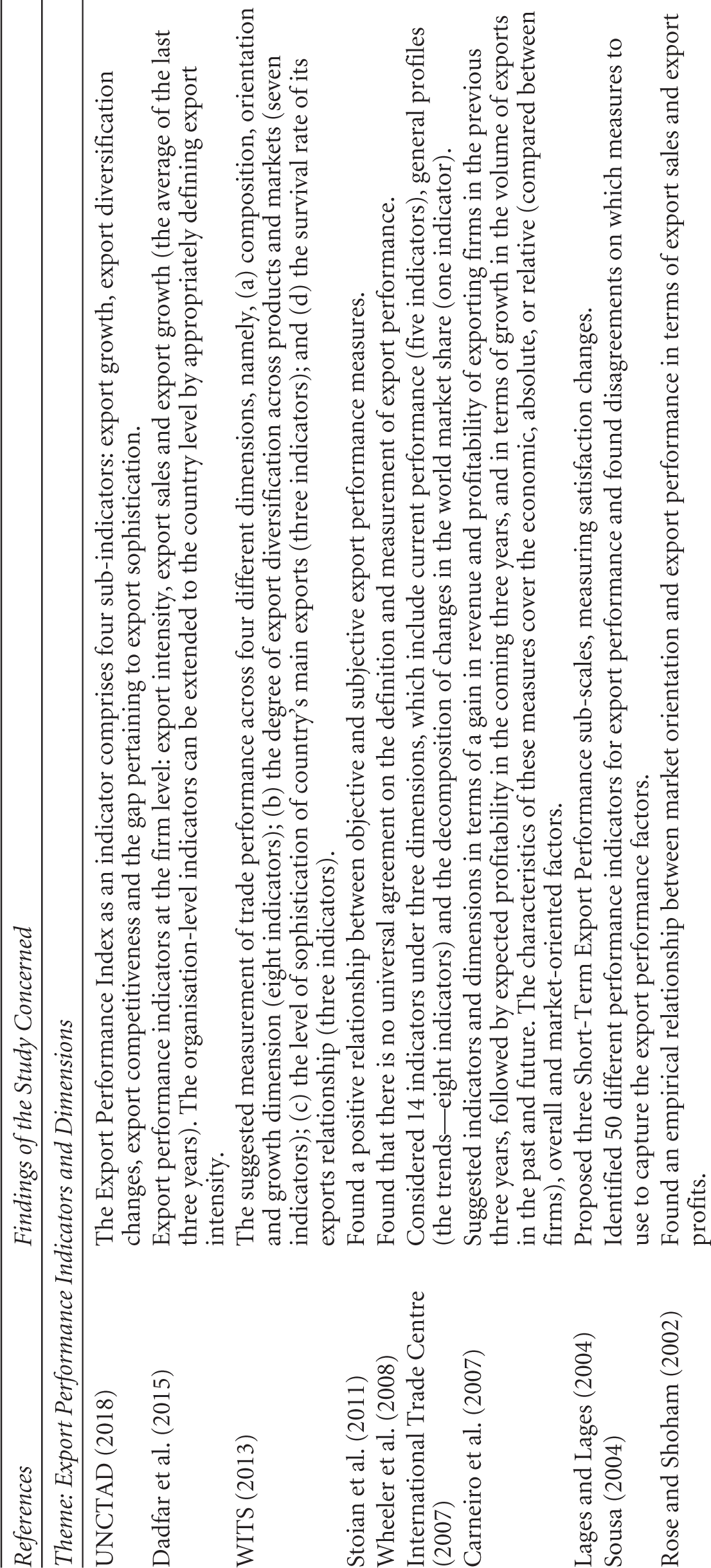
Several authors (Sousa, 2004; Wheeler et al., 2008; Zou & Stan, 1998) have pointed out that there has been no universal agreement on the definition and measurement of export performance. The lack of consensus on the dimensions and indicators within a dimension points to difficulties in measuring the multi-dimensional export performance and satisfying the desired properties from the measurement theory angle. For example, Sousa (2004) identified 50 different performance indicators for export performance and found disagreements on which measures to use for capturing the export performance factors. The author concluded that there was a need to develop a scale that enables comparison across countries.

The prevalent indicators often consider combinations of two or more variables, including percentage shares and growth rates. Combining the variables into indicators and selecting indicators may affect a country’s export performance. Diamantopoulos (1999) mentioned the need to include causal indicators in assessing export performance and the limitations of single-item measures due to their failure to completely capture the complex constructs. The performance dimensions of export firms can be extended to determine country-level performance (Walker & Rucket, 1987). Rose and Shoham (2002) found an empirical relationship between market orientation and export performance. However, openness alone is not a sufficient criterion (ITC, 2020). For example, openness per se does not measure export growth; it is only a driver for improvement in export performance.

Carneiro et al. (2007) reviewed 37 empirical articles and found that none of them satisfied the conditions of a sound framework and formative perspective. While considering over 100 export performance indicators, the authors suggested a set of indicators and dimensions in terms of gain in revenue and profitability of exporting firms in the previous three years, followed by expected profitability in the coming three years, and in terms of growth in the volume of exports in the past and future. The characteristics of these measures cover the economic, absolute, or relative (compared between firms), overall and market-oriented factors. However, the suggestions are not above criticism. The measures of some indicators are subjective. Thus, even if the above-listed issues are agreed upon, the problem remains as to how best to aggregate the indicators.

UNCTAD (2018) considered the Export Performance Index as an indicator with four sub-indicators, namely, export growth, changes in export diversification, export competitiveness and the export sophistication gap. The values of the sub-indicator of a country are predicted by a regression analysis, considering its level of per capita GDP, followed by an examination of the difference between this level and the country’s actual level, and ranking the countries accordingly. The authors used a weighted average of the ranks of each sub-indicator to define the overall positions of countries, using subjective judgement to select weights with the maximum weight assigned for export growth, moderate weight for export competitiveness and minimum (equal) weights for export diversification and the gap pertaining to export sophistication.

The methods of choosing weights differ significantly. The ratio of weights $\frac{W_{1}}{W_{2}}$ indicates the amount of indicator −2 that needs to be sacrificed to gain an extra unit of indicator −1. Thus, different weights lead to different interpretations. Therefore, there is a need to have an OEPI of countries considering all the relevant indicators and dimensions with appropriate aggregation methods without weights.

The Trade Performance Index (TPI) developed by the International Trade Centre (ITC) considered 14 sectors at the product level and calculated some indicators for each sector. WITS (2013) suggested the measurement of trade performance across four different dimensions, namely, (a) composition, orientation and growth dimension (eight indicators); (b) the degree of export diversification across products and markets (seven indicators); (c) the level of sophistication of the country’s main exports (three indicators); and (d) the survival rate of its exports relationship (three indicators). Shoham (1998) empirically found three dimensions of export performance after analysing 14 items and used Cronbach’s alpha to compute the scale’s reliability. However, the approach did not consider a single export venture. Subsequently, Shoham (1999) proposed two dimensions: export performance (the ratio of exports to total sales and the proportion of export sales to profitability) and a five-year change in export performance. However, this excluded market indicators and a formative structure.

Table 1 summarises the principal findings regarding export growth and performance measures under the following three different themes: ‘export performance indicators and dimensions’, ‘economy and trade’ and ‘methodology for export performance measurement’.

Table 1.

Export Growth and Performance

References	Findings of the Study Concerned
Theme: Export Performance Indicators and Dimensions
UNCTAD (2018)	The Export Performance Index as an indicator comprises four sub-indicators: export growth, export diversification changes, export competitiveness and the gap pertaining to export sophistication.
Dadfar et al. (2015)	Export performance indicators at the firm level: export intensity, export sales and export growth (the average of the last three years). The organisation-level indicators can be extended to the country level by appropriately defining export intensity.
WITS (2013)	The suggested measurement of trade performance across four different dimensions, namely, (a) composition, orientation and growth dimension (eight indicators); (b) the degree of export diversification across products and markets (seven indicators); (c) the level of sophistication of country’s main exports (three indicators); and (d) the survival rate of its exports relationship (three indicators).
Stoian et al. (2011)	Found a positive relationship between objective and subjective export performance measures.
Wheeler et al. (2008)	Found that there is no universal agreement on the definition and measurement of export performance.
International Trade Centre (2007)	Considered 14 indicators under three dimensions, which include current performance (five indicators), general profiles (the trends—eight indicators) and the decomposition of changes in the world market share (one indicator).
Carneiro et al. (2007)	Suggested indicators and dimensions in terms of a gain in revenue and profitability of exporting firms in the previous three years, followed by expected profitability in the coming three years, and in terms of growth in the volume of exports in the past and future. The characteristics of these measures cover the economic, absolute, or relative (compared between firms), overall and market-oriented factors.
Lages and Lages (2004)	Proposed three Short-Term Export Performance sub-scales, measuring satisfaction changes.
Sousa (2004)	Identified 50 different performance indicators for export performance and found disagreements on which measures to use to capture the export performance factors.
Rose and Shoham (2002)	Found an empirical relationship between market orientation and export performance in terms of export sales and export profits.
Redding and Venables (2002)	Export performance indicators include foreign market access and total exports.
Diamantopoulos (1999)	There is a need to include causal indicators in identifying export performance and the limitations of single-item measures due to their failure to capture the complex constructs completely.
Shoham (1999)	Proposed two dimensions: export performance (ratio of exports to total sales and the proportion of export sales to profitability) and a five-year change in export performance.
Zou et al. (1998)	Proposed a multi-dimensional scale to measure export performance. The dimensions are firm-level and include financial performance (related to exports in terms of profits, sales and growth), strategic orientation (in terms of the firm’s market share and similar) and the satisfaction dimension, that is, the perception of success of export ventures. However, the approach was faced with criticism (Diamantopoulos, 1999).
Shoham (1998)	Empirically found three dimensions of export performance after analysing 14 items and used Cronbach’s alpha to compute the scale’s reliability. However, the approach did not consider a single export venture.
Zou and Stan (1998)	Profitability is one crucial indicator and extends to country-level export performance.
Walker and Rucket (1987)	Suggested three dimensions for assessing any firm’s performance effectiveness (the firm’s market share), efficiency (output relative to the inputs employed) and adaptability (extent of response of the firm to the changing conditions and opportunities in the environment). These dimensions can get extended for use as a country-level export performance measure.
Theme: Economy and Trade
Chatterji et al. (2013)	Some indicators attempt to relate trade and economic growth because trade becomes more open as economies grow.
Ajmi et al. (2013)	Used a co-integration approach to establish a dynamic relationship between economic growth and trade variables using linear and non-linear Granger causality tests. However, rising inflation can constrain economic growth.
Yanikkaya (2003)	A positive association exists between trade openness and growth.
Lee and Huang (2002)	Export growth is a critical factor in promoting the economy.
Theme: Methodology
UNCTAD (2018)	Prediction of the values of a sub-indicator of a country by regression analysis considering its level of per capita GDP, followed by an analysis of the difference between this level and the country’s actual level and ranking the countries accordingly. Used a weighted average of the ranks of each sub-indicator to give the overall positions of countries using subjective judgement to select weights, according to the maximum weight for export growth, moderate weight for export competitiveness and minimum (equal) weights for export diversification and the gap pertaining to export sophistication.
Husein (2008)	Estimated critical parameters of the aggregate export demand function using annual time series data (1970–2004) and applying the Johansen–Juselius and Saikkonen–Lütkepohl multivariate co-integration procedures, and showed the empirical existence of a long-run equilibrium relationship among exports, foreign income, relative export price and domestic output.
Diamantopoulos and Kakkos (2007)	Opined that the export performance measure needs to be: (i) Composite and multi-dimensional, including both objective and subjective measures; (ii) have a frame of reference, that is, it needs to be benchmarked or compared; (iii) able to track the progress of a country across time; and (iv) able to detect critical areas requiring the attention of policymakers. The computation of the mean and variance of a group of countries could be an added advantage.
Morgan et al. (2004)	Used a seven-point Likert questionnaire for export venture performance in 17 constructed dimensions to assess the export venture performance outcomes.
Zou et al. (1998)	Developed an EXPERF scale using five-point Likert items and found three dimensions of export performance. The reliability of the questionnaire was estimated by Cronbach’s alpha despite getting many dimensions. Reliability by Cronbach’s alpha assumes a single dimension of the scale/questionnaire.

Source: Authors’ compilation.

2.2 Other Multi-dimensional Indices

Various studies have proposed multiple indices of a dimension and combined relevant indicators under the dimension. For example, in the family of indices for trade intensity, the index of Revealed Comparative Advantages (RCA), specifying pre-trade relative prices, is quite popular. However, the forms and uses of such indices vary over the traditional and present scenarios, where many countries are exporting a single commodity to different countries. In addition, a country may include imports for re-exports.

The Hillman Index (1980) emphasised monotonicity in the indices of RCA, while the Balassa Index (1965) defined it as follows:

\frac{Export of a country in a particular sector}{Total export of all countries in sector} \times \frac{1}{Ratio by the country's share of overall exports across all sectors}

The above equation reflects comparative advantage for cross-country comparisons (Redding, 2017). Researchers used the Hirschmann–Herfindahl Index (at the HS six-digit level) for export diversification, where lower values imply high diversification.

Cadot et al. (2011) found a U-shaped pattern of export diversification with an extensive database at the HS-6 level of disaggregation. Hallak (2006) considered unit values at the 10-digit level, followed by normalisation to arrive at a price index for each two-digit sector. This approach was modified by the International Monetary Fund by directly using unit values at the SITC four-digit level and substituting observables for the unobservable quality parameter in the gravity equation (Henn et al., 2013). Product concentration is assessed by the Sprade Index $(S_{cl}^{t})$ , which compliments equivalent number and is defined as $S_{cl}^{t} = \frac{\sqrt{\sum_{k = 1}^{cl} {(X_{i \cdot k}^{t} - \bar{X_{l \cdot cl}^{t}})}^{2}}}{N \cdot \bar{X_{l \cdot cl}^{t}}}$ where $X_{i \cdot k}^{t}$ denotes exports of product k from ith country to market i in the tth year, and $\bar{X_{l \cdot cl}^{t}}$ indicates the average value of country i exports in year t for the cluster cl. However, the index is not invariant under a change of scale.

UNCTAD came out with a database of Revealed Factor Intensity Indices (RFII) of products at the HS six-digit level of product classification based on the study by Cadot et al. (2010). RFII approximates the revealed factor content of a product as a weighted average of the factor endowments of countries exporting the product, where the weights represent the exporters’ RCAs (Nicita et al., 2013). Based on the micro-foundations of a country’s competitiveness, Porter et al. (2004) suggested a microeconomic index of competitiveness that correlates with per capita income. Carneiro et al. (2007) considered export performance as a dependent variable to identify the indicators. However, the problem remains to measure the overall export performance by suitably aggregating the chosen dimensions and indicators within a dimension.

Assessing overall export performance and comparing two countries at a time or one country at two different periods necessitates combining the selected indicators in a meaningful way. Defining a function f combining n-indicators to an OEPI will be a real number. Different approaches are suggested for obtaining such a function to obtain the OEPI.

Unfortunately, there is no agreement on the aggregation of chosen indicators to a single measure of export function. Attempts to combine the indicators or dimensions as a weighted sum also differ in terms of selecting weights and may not be free from bias.

The present state of affairs does not allow meaningful comparisons of OEPI over time or space or tracking of the path registered by a country to improve overall performance through initiatives taken or policy measures adopted and comparisons concerning such paths. Therefore, constructing a meaningful and sound index with the desired properties is the focus area rather than the ranks or rank robustness.

2.3 Review of the Index Development Methodology

2.3.1 Nature of Data and Limitations

The indicators could be absolute or relative. For example, the normalised trade balance of a country is defined as $\bar{TB} = \frac{X - M}{X + M}$ where X denotes export value, and M represents import value. The indicator compares (X – M)with the trade value of a country as the standard. Thus, it may be difficult to compare the two countries since the standards are different. Two countries with an equal value of (X – M) may have different normalised trade balance values. Consider the following example: Let the export value of countries A and B be X_A and X_B, respectively. Define M_A and M_B as the import values of A and B, respectively. Consider the situation where X_A = 512, M_A = 500, and X_B 1610, M_B = 1598. Here, X_A – M_A = X_B – M_B = 12. But, ${\bar{TB}}_{A} > {\bar{TB}}_{B}$ . An illustrative list of other relative indicators is the trade balance in goods and services as a percentage of GDP, defined as TB–GDP = $\frac{X - M}{GDP} \times 100;$ trade-to-GDP ratio = $\frac{X + M}{GDP} \times 100,$ trade per capita = $\frac{X + M}{N}$ where N denotes the number of inhabitants.

Foreign trade balances (exports minus imports of goods and services) may be negative for countries with a deficit or positive for countries with a surplus.

Indicators may be biased by the country’s size (both in terms of GDP and geographical size). For example, indicators on trade openness based on GDP, and trade balance in goods and services as a percentage of GDP; export propensity = $\frac{X}{GDP}$ . The net trade indicator (X – M) is also biased across time, countries and sectors.

Indicators may be in percentages, for example, FDI indicators like FDI flow as a percentage of GDP; and technology-based indicators like technology payments and receipts as a percentage of GDP, among other things. The other indicators in percentages are as follows: share of a country in the world market; relative trade balance; export growth in value in percentage is the compounded annual growth rate of exports, usually during the last five years. The competitiveness effect shows the percentage change in the competitiveness of a country’s exports globally for the selected sector in the period under review. This indicator is defined as a change in the exporting country’s share in the destination markets’ imports times the initial share of partner countries’ imports in world trade (weighted average of the variation in the country’s position on elementary markets). Averaging figures in percentages may distort the result, especially if the denominators are not multiples of the others.

Indicators may reflect the geographical concentration of a country’s exports or imports. For example, the Herfindahl index of geographical concentration for country A’s exports is the sum of the squares of the market shares held in each destination country. Note that the concentration can vary significantly by the type of goods.

Various indicators make different assumptions for their purposes. For example, the same elasticity of substitution for domestic and foreign firms within sectors is assumed by Redding (2017). Caliendo and Parro (2015) considered the same unit expenditure function for final consumption and intermediary uses within each industry. However, researchers differed regarding assumptions on shifts in demand/quality. While the Sato–Vartia price index assumes no changes in demand/quality for surviving varieties, price indices with time-varying demand/quality assume the opposite.

2.3.2 Correlations among Indicators

Indicators have correlations of varying degrees. For example, the correlation between the coverage ratio (CR) = $\frac{X}{M} \times 100$ and net trade indicator $(\bar{NT} = X - M)$ is 1 since $\bar{NT} = \frac{CR - 1}{CR + 1}$ . Similarly, the correlation between TB–GDP and trade-to-GDP ratio (also known as the Trade Openness Ratio) is perfect. Export efficiency indicators are highly correlated with export sales indicators and indicators relating to export proﬁtability. The inclusion of highly correlated indicators results in multicollinearity.

The correlation between subjective indices also varied. For example, Stoian et al. (2011) found that managers’ knowledge of international business had a maximum correlation (0.363) with firm export commitment and a minimum (−0.220) with managerial perceived export barriers.

2.3.3 Indicators as Weighted Sum or Logarithm of Variables

So far, researchers have proposed indices based on weights, such as the export performance as the ratio of total exports and export market, where the authors determined export markets based on a weighted average of import volumes in each country. The authors propose weights based on trade flows in time t. The formula is ${EP}_{i}^{t} = Δ X_{i}^{t} - \sum_{i - 1}^{n} α_{i} Δ M_{i}^{t}$ , where $\frac{Δ X_{i}^{t}}{Δ M_{i}^{t}}$ is the export growth rate of the ith country in period t/import growth rate of the market in tth period and a_i is the weight of the ith market. Different choices of weights will give different results even if the sum of weights is equal to unity. Hargreaves et al. (1993) considered the Competitive Index of Australia as $\frac{\sum (P_{j} E_{j}) W_{j}}{P_{a} E_{a}}$ where E_a and E_j are the nominal exchange rates for Australia and the jth country, respectively, P_a and P_j are the equivalent price (or cost) index for Australia and the jth country, and W_ij is the weight assigned to the jth country and reflects the country’s importance in trade with Australia alone or on the world market of the chosen set of commodities for exports and the domestic market for imports. Thus, the weighting system may vary.

The gravity equation is a regression equation that considers the logarithm of exports from ith to jth country (X_ij) as the dependent variable; the independent variables comprise the logarithm of the bilateral distance, bilateral trade cost, market capacity of the export partner and supply capacity. The logarithm of supply capacity is obtained by regressing with the logarithm of variables such as GDP, population, internal transport costs and a set of institutional and macroeconomic variables (relevant to export sector competitiveness) (Redding & Venables, 2004). Taking the logarithm of a variable and another variable (without logarithm) in the set of independent variables may lower the weights of the variables expressed in the logarithm. However, the wide variety of methodological approaches to weighting and aggregation introduces subjectivity and often uncertainty (Rowley et al., 2012).

A possible solution to the above could be to consider the ratio of each indicator (irrespective of type, score range and correlation pattern) in the current period and base period, and use the appropriate formula to aggregate such ratios. The aggregation may be a function of the geometric mean (GM), avoiding normalisation of variables, and selecting weights for indicators.

2.3.4 Subjective Indicators

The subjective indicators based on the Likert scale, such as satisfaction or perceived success of the venture, changes in satisfaction and export venture performance, among other things, are discrete and ordinal. Following are the other problems associated with Likert data:

It is not additive as the distance between levels is unequal and unknown (Ferrando, 2003; Wu, 2007).

Scales are generally not perceived as equidistant by the subjects (Lee & Souter, 2010).

Assumption of equal importance to the items for the summative Likert scores may not be justified because of the different values of correlations between items, item and total score, and different factor loadings.

Non-satisfaction of the equidistance assumption implies non-admissibility of operations like averaging. Therefore, the analysis must be limited to frequencies under the item–response category combinations.

$\bar{X} > \bar{Y}$ could be meaningless as strictly speaking, the arithmetic mean (AM) is not defined for ordinal scales (Hand, 1996). The use of the mean and SD for ordinal scales was not favoured by Jamieson (2004).

Do not consider patterns of getting a particular score. Different responses to different items can generate identical Likert scores for more than one respondent. Thus, the scale fails to discriminate between the respondents with the same Likert scores.

Considering the anchor value of zero in the Likert items, mis-states the AM, variance, skewness and kurtosis (Dawes, 2002). The incidence of zero responses to an item in large numbers artificially lowers the associated co-variance and correlation. The analysis involving numerical values attached to the levels (like expected values) may not be meaningful because zero is attached to a level.

The numerical values attached to the response categories of Likert items may be −3, −2, −1, 0, 1, 2 and 3. Hypothetically, if 50 per cent of the respondents endorse −3, and the rest 50 per cent endorse 3, the average will be zero, implying that the group is neutral against the reality of a polarised group. A possible solution could be to allot numbers 1 to 7 to the categories as a linear transformation does not change the data. If all the respondents endorse a particular response category, the variance of that item is zero, which implies that the inter-item correlations and item-total correlation involving that item are undefined.

The distributions of item scores and test scores are different and often found to be skewed.

Morgan et al. (2004) used a seven-point Likert scale for assessing managerial satisfaction. On the other hand, the EXPERF scale used a five-point scale (Zou et al., 1998). Therefore, the following question arises: How can we link responses in a K-point scale with (K + J)-point scale where J = 1, 2, 3,…, and so on?

Items in Likert scales may have an equal number of response categories (say a five-point scale) or a combination of three-point, four-point, five-point and seven-point scales, which differ in mean and SD. The response categories influence item/test parameters more than the respective variable (Lim, 2008). The mean and variance increase with several categories in the rating scale (Finn, 1972). Different categories lead to different reliability, validity and discriminating power of the scale (Preston & Colman, 2000).

Correlations between ordinal Likert data and secondary variables, in ratio scales such as GDP, trade balance, export propensity and similar, are not possible for a particular year of a country.

Possible solution: The Likert scores need transformation to satisfy the desired properties such as interval or ratio scale of measurement, continuous data, monotonic and admissibility of addition, among others. Chakrabartty (2019) proposed converting scores of responses obtained by using a Likert scale to a ratio scale to ensure that the scores are monotonic and equidistant, and evade ties.

2.3.5 Selection of Indicators

The indicators could be a single variable or more than one variable. Many criticisms highlight the exclusion of one or more indicators/dimensions. For example, while reviewing the impact of trade liberalisation and exchange rate, Santos-Paulino and Thirlwall (2004) have ignored factors such as natural barriers, the availability of infrastructure and market access in explaining export performance. The approaches and methods vary even for the same indicator. There is no agreement in the set of indicators for measuring the Overall Performance Index for export. The indicators and dimensions of export performance may be categorised in terms of financial/economic, non-financial/non-economic and composite measures. The assessment types may be objective or subjective, or a combination of both. The indicators may be absolute or relative, with each of them attempting to assess one or more dimensions.

The choice of indicators and dimensions needs to ensure that:

It explains the dynamics of exports.

There are adequate reasons for its inclusion.

It avoids bias across time, countries and sectors.

It avoids or minimises multicollinearity.

It ensures at least the interval level measurement of each indicator.

Each chosen indicator is positively related to the OEPI, as it should be increasing monotonically. If the indicators on inflation, trade barriers and other similar factors are chosen, which are negatively associated with OEPI, their reciprocal may be considered.

Hence, the study needs to avoid the limitations mentioned above.

2.3.6 Combining the Indicators

This is probably the most crucial stage. Combining the indicators, that is, to find the function from Rⁿ → R, corresponding to n-indicators can affect the properties and further operations to OEPIs, and may significantly impact the ultimate index. ITC (2020) found a Composite Index based on the simple average of five rankings of the current five performance indicators. The limitations of such arithmetic average are as follows:

It assumes that all indicators are equally important, which may not be valid. For example, a share in the world market, the value of net exports, product concentration and market concentration, among other things, may not be equally important and may have different correlations with the OEPI. Besides, the correlation between a pair of selected indicators also varies.

The interpretation of the addition results may be difficult since the chosen indicators have different distributions. The addition of data in percentages can provide an incorrect result when the denominators are non-multiple. For example, if 80 per cent (16 out of 20) and 40 per cent (as 4.8 out of 12) are pooled, the result is 65 per cent, which is not equal to 60 per cent (average of 80 per cent and 40 per cent). However, the ratio (that is, the division) of two indicators in percentages is admissible.

It assumes perfect substitutability among the indicators. Thus, a low-level value of one indicator may be compensated by a high-level value of another indicator.

The unobservable overall performance (Y) may be estimated by combining the chosen indicators as a weighted sum where weights were found through principal component analysis (PCA) of the standardised component indicators. The estimate of $E (\frac{Y}{X_{1}}, X_{2}, ..., X_{n})$ is $\frac{\sum_{i = 1}^{n} λ_{i} P_{i}}{\sum_{i = 1}^{n} λ_{i}}$ , where m₁ is the first characteristic root of the correlation matrix R. Other m’s are defined accordingly. Here, m₁ > m₂> … > m_n and corresponding characteristic vectors of R are (a₁, a₂, …, a_n)^T The n—principal components of the indicators are: P₁, P₂, …, P_n where $P_{1} = \frac{α_{11} (X_{1} - \bar{X_{1}})}{S_{1}} + \frac{α_{12} (X_{2} - \bar{X_{2}})}{S_{2}} + \dots + \frac{α_{1 n} (X_{n} - \bar{X_{n}})}{S_{n}}$ , P₂, …, P_n are defined accordingly. The asymptotic distribution of the estimate of Y was given by Nagar and Basu (2004) for n = 2, when the number of observations tends to be large.

The problems of weights through PCA are as follows:

Variance and covariance are not invariant under the change of scale.

Weights from PCA ignore or poorly weigh the indicators that do not strongly correlate with the overall performance even if they are theoretically and practically significant.

Weights depend on data. Thus, the PCA weights may vary for data for different years.

2.3.7 Desired Properties

The desired properties of an aggregation function to get a single value of the OEPI are as follows:

P₁: OEPI to reflect the position of a country by a continuous variable;

P₂: monotonically increasing, that is, gain in an indicator (X_i) to result in the gain of OEPI;

P₃: $\frac{Gain i n O E P I}{Gain i n X_{i}}$ to be constant, that is, X–OEPI curve to be linear;

P₄: homogeneity, that is, independent of the change of scale;

P₅: identification of key indicators, where performances have not increased and require the attention of the policymakers;

P₆: satisfy the time-reversal test, that is, OEPI_C0 ×OEPI_0C = 1, where OEPI_C0 is the index of the overall performance of a country at period C with respect to the base period;

P₇: quantification of progress made by a country over time, which in turn, helps drawing the path of progress/decline of a nation; and

P₈: facilitates computation of the mean and variance of OEPI for a group of countries at a given time.

3. Proposed Overall Export Performance Index (OEPI)

3.1 Data Pre-processing

The authors propose the pre-processing of data before the computation of OEPI. First, the authors suggest the conversion of each indicator such that all indicators are related positively to the OEPI, that is, if any indicator is negatively associated, its reciprocal is taken before processing. In the subjective measures (if any), the responses are obtained using a Likert scale with an equal number of response categories. First, the discrete summative scores are converted to continuous, monotonic and equidistant scores. Then each Likert item is equi-correlated with the test score. The four-stage approach suggested by Chakrabartty (2019b) is described below.

First, the response categories of the Likert items are assigned with numbers beginning with 1, avoiding zero, to facilitate meaningful operations. The second step is the generation of continuous scores converting raw scores to equidistant scores by assigning data-driven weights to the response categories. This conversion satisfies the monotonic condition (to assess the progress or otherwise), equidistant property (to facilitate addition) with zero ties (to distinguish amongst respondents with the same raw score) and specifies zero value for scoring Likert items as a weighted sum. Third, the standardised equidistant scores (X) of each item are taken as $Z = \frac{X - \bar{X}}{SD (X)}$ . Fourth, the equi-correlated property is satisfied, that is, making test scores equi-correlated with the items by assigning weights to items, thus justifying the addition of converted item scores.

In cases of different responses in the Likert scales (three-point or four-point or five-point scale, or so on), the authors propose to apply the first three steps of the approach suggested by Chakrabartty (2019b) separately on each sub-test of the different k-point scales, where k = 3, 4, 5, 6, 7, or so on. Then, the scores are transformed to have the proposed mean and SD and added to get the sub-test and test scores. The sub-test scores obtained in this fashion will be normally distributed with the same mean and variance for all the k-point scales and attain comparable results.

3.2 Methodology

Let X_it > 0 be the value of the ith indicator for the tth period of a country, obtained after the data pre-processing presented above. For the base period, the corresponding value is X_i₀. The chosen indicators could be independent or correlated with varying degrees. The ratio $\frac{X_{i t}}{X_{i 0}}$ is unit free and indicates the progress or decline of the country for the ith indicator at the tth time over the base period. The value of $\frac{X_{i t}}{X_{i 0}} > 1$ indicates the extent of progress and $\frac{X_{i t}}{X_{i 0}} < 1$ indicates the degree of decline with respect to the ith indicator. The OEPI of a country for the tth period is proposed to be taken as:

{OEPI}_{t} = \prod \frac{X_{i t}}{X_{i 0}} for i = 1, 2, 3, ..., n

(1.1)

For general convention, the OEPI_t maybe multiplied by 100 to reflect the percentage OEPI_t.

Properties:

Equation (1.1) is the nth root of the GM of n-number of ratios $\frac{X_{i t}}{X_{i 0}}$ . Thus, GM has a one-to-one correspondence with Equation (1.1).

It is simple and considers all the chosen indicators, including those in percentages, and depicts an overall improvement/decline in the current year corresponding to the base year in a unit-free fashion, avoiding scaling scores and selecting weights.

OEPI > 1 implies an overall improvement from the base year.

It identifies the critical areas requiring attention in terms of the ratios for which $\frac{X_{i t}}{X_{i 0}} < 1.$

It reduces the level of substitutability between the component indicators.

It finds the relative importance of indicators. However, the contribution of an indicator may vary with time.

It is independent of the change of scale and gives a continuous function, which increases monotonically. An increase of 1 per cent in X_it implies a 1 per cent increase in the OEPI, if all other factors remain unchanged. In other words, the curve showing a gain in an indicator and gain in OEPI is linear, that is, the OEPI has constant elasticity.

It satisfies the time-reversal test as OEPI_t0 . OEPI_0t =1.

Chain indices can be formed as OEPI₂₀ = OEPI₂₁ . OEPI₁₀.

It is possible to draw the OEPI graph of a country over a long period to reflect the path of improvement/decline over time.

The similarity between two OEPI graphs of two countries covering years 1, …, t can be found considering the Euclidian distance between the two t-dimensional vectors I₁ = (I_1,1, I_1,2, …, I_1,t)^T and I₂ = (I_2,1, I_2,2, …, I_2,t)^T However, distance emphasises larger differences between the respective components of two vectors. A better measure of similarity between two vectors of the same dimension is given by the cosine similarity between the vectors I₁ and I₂ as

Cos θ_{12} = \frac{I_{1}^{T} I_{2}}{‖ I_{1} ‖ ‖ I_{2} ‖}

(1.2)

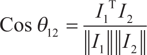
where I_ij is the OEPI-value of the ith country for the jth year [i = 1, 2 and j = 1, 2,…,t], $‖ I_{1} ‖$ and $‖ I_{2} ‖$ are the length of the vectors I₁ and I₂ respectively, and i₁₂ is the angle between I₁ and I₂. Here, 0 ≤ Cos i₁₂ ≤ 1. A measure of dissimilarities of the OEPI between two countries may be depicted by Sin i₁₂, where Sin i²₁₂ = 1 − Cos i²₁₂.

If the OEPI values are obtained for the k number of countries where k is large, a natural question arises regarding the average of OEPI of the world. The same can be answered by finding the average and dispersion of $cos {θ^{'}}_{i j} s,$ following the method suggested by Rao (1973) to find the mean and dispersion of angles $\emptyset_{1}, \emptyset_{2}, \dots, \emptyset_{k}$ , with each obtained for vectors of unit length as follows:

The mean or most preferred direction is

\bar{\emptyset} = {Cot}^{- 1} \frac{\sum_{i = 1}^{k} cos \emptyset_{i}}{\sum_{i = 1}^{k} sin \emptyset_{i}}

(1.3)

and the dispersion is given by

\sqrt{1 -} r^{2} where r^{2} = {(\frac{\sum cos \emptyset_{i}}{k})}^{2} + {(\frac{\sum sin \emptyset_{i}}{k})}^{2}

(1.4)

It was not affected much by extreme values (outliers) and thus produced no bias for the developed or under-developed countries.

It is possible to compute separate indices for each dimension by focusing on a sub-set of indicators related to that dimension without requiring further weights for dimensions.

It is possible to find the mean of OEPI for a group of countries by considering the log(100•OEPI).

It is possible to satisfy all the desired properties, P₁ to P₈ mentioned earlier.

3.3 Applications of OEPI

The proposed index can be constructed even for skewed longitudinal data over long and two time periods. Thus, it helps in a meaningful comparison of the overall export performance of a set of countries.

It offers a simple solution to assess the OEPI even at the individual country level from the base period without resorting to data for a group of countries. Thus, it helps to find the OEPI of a country while considering data for the particular country only.

It can be well used for the ranking and classification of countries.

It is possible to find the average OEPI for a group of countries.

The graph of progress or decline of the OEPI using the chain indices obtained from the proposed index over time for a country will help assess the impact of various strategic decisions. ${OEPI}_{i_{t}} > {OEPI}_{i_{(t - 1)}}$ or $\frac{{OEPI}_{i_{t}}}{{OEPI}_{i_{(t - 1)}}} > 1$ will indicate progress made by the ith country in period t over (t − 1)th period.

The critical indicators where deterioration occurred can also be identified by observing those for which $\frac{X_{i t}}{X_{i (t - 1)}} < 1$ and may be used for policy purposes to decide appropriate action plans.

4. Empirical Verification

4.1 Computation of OEPI

The feasibility of computation of a proposed measure of OEPI and investigation of satisfaction of significant properties of the measure have been illustrated; data on five country-level indicators were obtained from the WITS (WITS, 2020) for the USA and India for the period 2014 to 2018. The chosen indicators are detailed below.

X₁: HH Market Concentration Index = $(\sqrt{{\sum_{j = 1}^{N} (\frac{X_{i, j}}{X_{j}})}^{2}} - \sqrt{\frac{1}{N}}) \div (1 - \sqrt{\frac{1}{N}})$

where X_ij is the value of exports of the ith product by jth country; X_i denotes the world value of exports of the ith product and N is the total number of exporting countries.

The index ranges from [0, 1], with a large value indicating a higher concentration in the export market.

X₂: Index of Export Market Penetration of exports of country j = $\frac{\sum_{i = 1}^{N} (X_{i, j})}{\sum (X_{i, w})}$

where X_ij is the value of the ith product of jth country, X_i_{, w} is the total value of the world exports of the ith product and N is the total number of exporting countries.

The indicator measures how a country’s exports reach already proven markets. A low value of the index may be due to barriers to trade preventing an expansion of the number of markets to which they export.

X₃: Reciprocal of HH Product Concentration Index. Let us first consider the HH Product Concentration Index, which is defined as $\frac{\sqrt{\sum_{i = 1}^{N} {(\frac{X_{i, j}}{X_{j}})}^{2}} - \sqrt{\frac{1}{N}}}{1 - \sqrt{\frac{1}{N}}}$ , where the notations are the same as those indicated in X₁. Like X₁, the HH Product Concentration Index also varies between 0 and 1, where the value of 1 implies that all exports of the jth country came from a single commodity, which is not desirable for a country. Accordingly, the reciprocal of the HH Product Concentration Index was chosen as an indicator so that it is positively related to OPEI.

X₄: Number of Export relationships = Number of export partners with trade

values of at least 10,000 USD each year.

The country with the ability to maintain or enhance trade relationships is seen as a better performer in exports. This number is suitably converted into a ratio reported in the WITS database as ‘Export-Duration’ under the Export-Survival indicator.

X₅: Export as a percentage of total trade = $\frac{Value of export}{Value of import + value of export} \times 100$

4.2 Ratio of Current Year Value and Base Year Value

Table 2 shows the data for each chosen indicator for the USA and India from 2014 to 2018.

Table 2.

Values of Chosen Indicators for the USA and India

Indicators		Values of Indicators
Indicators		2014	2015	2016	2017	2018
HH market concentration index (X₁)	USA	0.05983542	0.0596176	0.05800198	0.05791452	0.05832396
HH market concentration index (X₁)	India	0.04356593	0.04987978	0.05251539	0.04724562	0.0549913
Index of export market penetration (X₂)	USA	47.1033335	45.3081351	44.8051182	44.8651659	40.1030126
Index of export market penetration (X₂)	India	28.2460717	28.1223501	28.6192259	29.52653	27.1453618
Reciprocal of HH product concentration index (X₃)	USA	109.89011	153.846154	158.730159	135.135135	114.942529
Reciprocal of HH product concentration index (X₃)	India	21.7391304	41.322314	43.1034483	40.9836066	32.0512821
Index of export relationships (X₄)	USA	14	10	11	12	11
Index of export relationships (X₄)	India	95	55	49	51	63
Export as a percentage of total trade (X₅)	USA	0.40186164	0.39364074	0.39234111	0.39123661	0.38938648
Export as a percentage of total trade (X₅)	India	0.40872555	0.40355765	0.421902	0.39864271	0.34277688

Source: WITS (http://wits.worldbank.org/WITS/WITS/AdvanceQuery/TradeOutcomes/IndicatorDefinition.aspx?Page=Indicator).

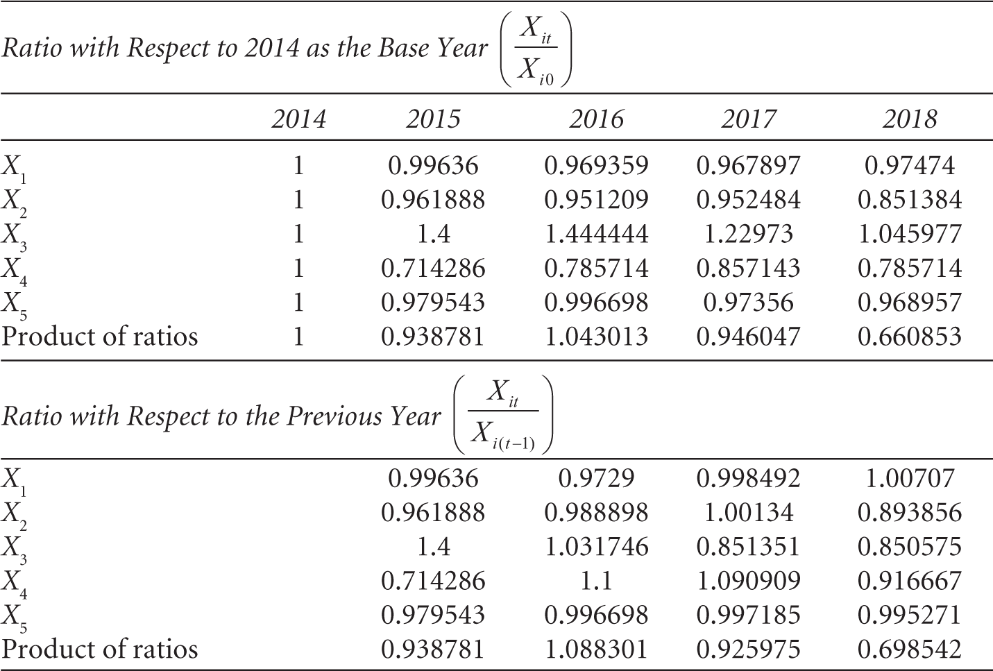
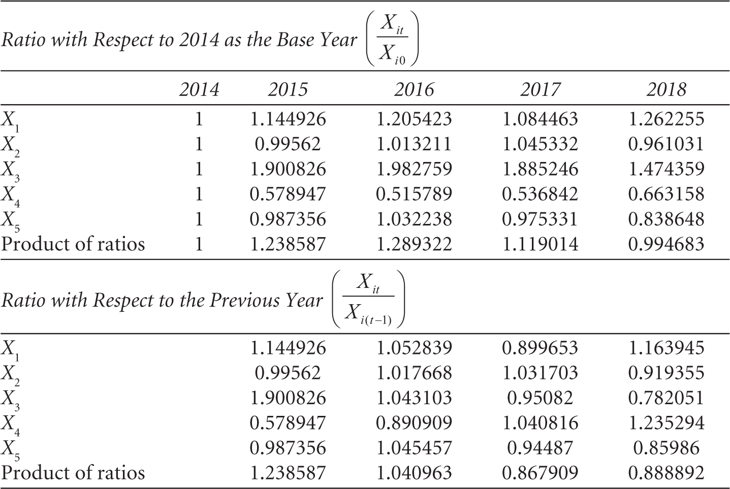
Tables 3 and 4 show the ratios with respect to 2014 (considered as the base year) and year-on-year (Y-o-Y) ratios for the USA and India, respectively.

Table 3.

Ratio of Indicators with Respect to 2014 and Y-o-Y Ratios for the USA

Ratio with Respect to 2014 as the Base Year $(\frac{X_{i t}}{X_{i 0}})$
	2014	2015	2016	2017	2018
X ₁	1	0.99636	0.969359	0.967897	0.97474
X ₂	1	0.961888	0.951209	0.952484	0.851384
X ₃	1	1.4	1.444444	1.22973	1.045977
X ₄	1	0.714286	0.785714	0.857143	0.785714
X ₅	1	0.979543	0.996698	0.97356	0.968957
Product of ratios	1	0.938781	1.043013	0.946047	0.660853
Ratio with Respect to the Previous Year $(\frac{X_{i t}}{X_{i (t - 1)}})$
X ₁		0.99636	0.9729	0.998492	1.00707
X ₂		0.961888	0.988898	1.00134	0.893856
X ₃		1.4	1.031746	0.851351	0.850575
X ₄		0.714286	1.1	1.090909	0.916667
X ₅		0.979543	0.996698	0.997185	0.995271
Product of ratios		0.938781	1.088301	0.925975	0.698542

Source: WITS. (http://wits.worldbank.org/WITS/WITS/AdvanceQuery/TradeOutcomes/IndicatorDefinition.aspx?Page=Indicator) and authors’ work.

Table 4.

Ratio of Indicators with Respect to 2014 and Y-o-Y Ratios for India

Ratio with Respect to 2014 as the Base Year $(\frac{X_{i t}}{X_{i 0}})$
	2014	2015	2016	2017	2018
X ₁	1	1.144926	1.205423	1.084463	1.262255
X ₂	1	0.99562	1.013211	1.045332	0.961031
X ₃	1	1.900826	1.982759	1.885246	1.474359
X ₄	1	0.578947	0.515789	0.536842	0.663158
X ₅	1	0.987356	1.032238	0.975331	0.838648
Product of ratios	1	1.238587	1.289322	1.119014	0.994683
Ratio with Respect to the Previous Year $(\frac{X_{i t}}{X_{i (t - 1)}})$
X ₁		1.144926	1.052839	0.899653	1.163945
X ₂		0.99562	1.017668	1.031703	0.919355
X ₃		1.900826	1.043103	0.95082	0.782051
X ₄		0.578947	0.890909	1.040816	1.235294
X ₅		0.987356	1.045457	0.94487	0.85986
Product of ratios		1.238587	1.040963	0.867909	0.888892

Source: Authors’ computation.

5. Results and Discussion

5.1 Results

The values of $\frac{X_{i t}}{X_{i 0}} > 1$ indicate an improvement in the performance of the ith indicator in the current period over the base year. Here, $\frac{X_{3, t}}{X_{30}} > 1$ for the indicator X₃ in 2015, 2016, 2017 and 2018 for the USA. However, for India, each of X₁ and X₃ improved during 2015, 2016, 2017 and 2018; X₂ improved in 2016 and 2017; and X₅ improved in 2016 only. Thus, the increasing trends in terms of improvement over the base year were seen more for India than the USA.

5.1.1 Critical Areas

The critical areas for a country require managerial attention for possible changes in policy measures. The critical areas are those indicators having $\frac{X_{i t}}{X_{i 0}} < 1$ or those with $\frac{X_{i t}}{X_{i (t - 1)}} < 1$ . Therefore, it may be prudent to consider critical areas as the indicators that satisfy the two above-mentioned inequalities. Accordingly, critical areas that emerged from the data are given in Table 5.

Table 5.

Critical Areas for the USA and India

Country		2015	2016	2017	2018
USA	X ₁	✓	✓	✓	✓
	X ₂	✓	✓		✓
	X ₃
	X ₄	✓			✓
	X ₅	✓	✓	✓	✓
India	X ₁
	X ₂	✓			✓
	X ₃
	X ₄	✓	✓
	X ₅	✓		✓	✓

Source: Authors’ computation.

Note: The number of critical areas for India was much less (35 per cent) than that for the USA (65 per cent).

5.1.2 Computation of OEPI

The OEPI for a country for a year was computed by considering the ratios with respect to (w.r.t.) the base year, that is, 2014 (Approach 1), and separately considering the ratios with respect to the previous year (Approach 2). The OEPI figures for the USA and India were computed using Approach 1, as shown in Table 6.

Table 6.

OEPI by Approach 1 for the USA and India

OEPI Values by Approach 1
	2014	2015	2016	2017	2018
USA	1	0.938781	1.043013	0.946047	0.660853
India	1	1.238587	1.289322	1.119014	0.994683

Source: Authors’ computation.

Figure 1 indicates a higher growth trend of OEPI for India as compared to the USA.

Figure 1.

Source: Authors’ computation.

Figure 2.

Source: Authors’ computation.

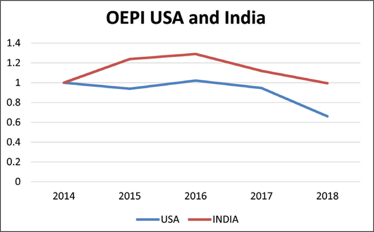
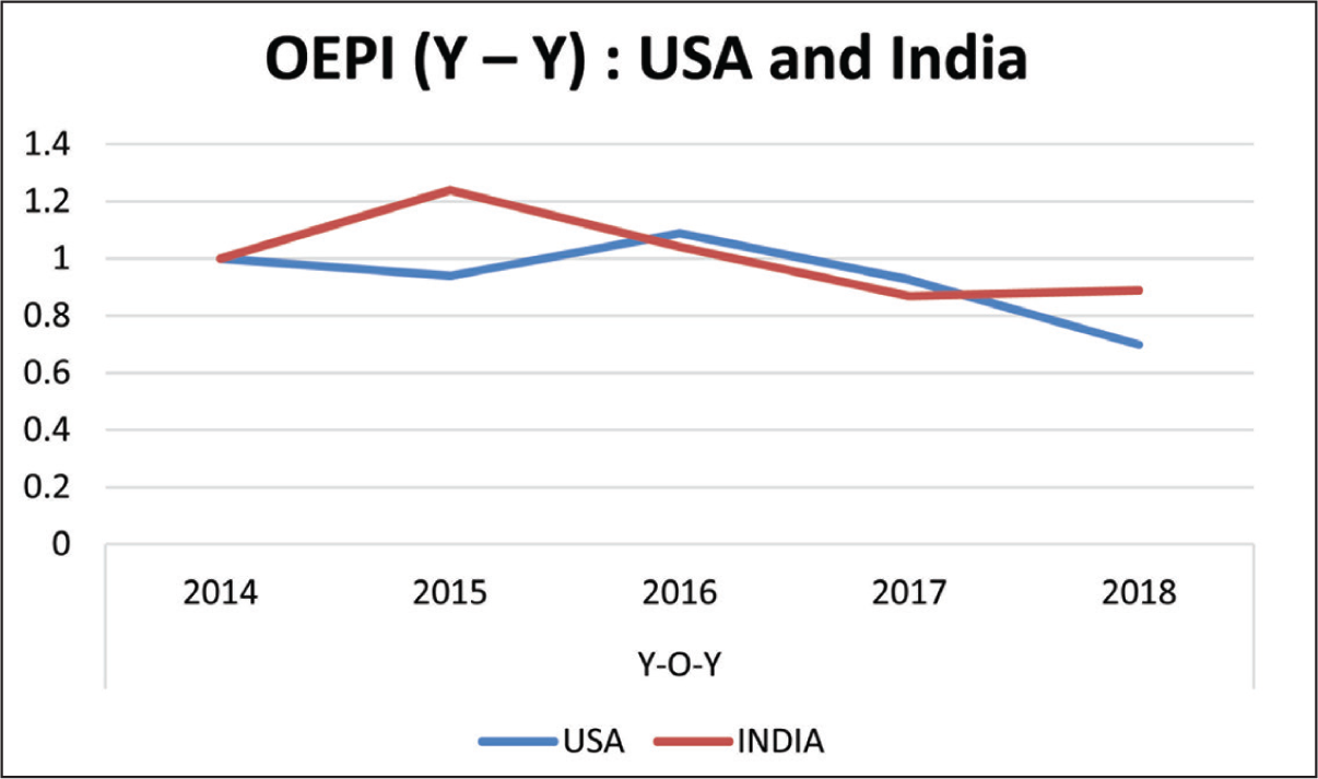
Table 7 shows the Y-o-Y growth of the two countries’ overall export performance index (Approach 2).

Table 7.

OEPI by Approach 2 for the USA and India

	2015	2016	2017	2018
USA	0.938781	1.088301	0.925975	0.698542
India	1.238587	1.040963	0.867909	0.888892

Source: Authors’ compilation.

Note: The trends shown in Figure 2 indicate the Y-o-Y growth for India as compared to that for the USA from 2015 to 2018.

After registering steady growth in 2016, the OEPI for the USA declined in 2017 and further dropped in 2018. The OEPI for India reached the top in 2015 and fell after that till 2017. It registered improving trends in 2018.

Observations:

Approach 2 showed more fluctuations in OEPI than Approach 1. This indicates that Approach 1 for finding the OEPI of a country gives more stable figures than the other approach. Besides, the base-year analysis allows for a comparison between the current performance and historical performance and provides a broader canvas for planning in the long run. The use of Approach 1 may ignore fluctuations in the values of the volatile indicators on a Y-o-Y basis.

A volatile indicator (the presence of which can be seen from the high value of SD of the indicator in past data) is likely to fluctuate more. Therefore, the ratio of such a volatile indicator with the base year may affect the OEPI value.

5.1.3 Relative Importance of Indicators to OEPI

The contribution of the ith indicator to the OEPI of a country in a year was approximated by $\frac{X_{i t, Country A}}{{OEPI}_{t, Country A}},$ keeping in mind that it may exceed 1. Further, the ranks based on the five indicators (by Approach 1) were assigned separately for India and the USA each year (other than in 2014). The average ranks of the indicators for India and the USA gave their relative importance to OEPI. Empirically, the ranks of the indicators were as follows: X₄: rank I, X₂: rank II, X₅: rank III, X₁: rank IV and X₃: rank V.

5.1.4 Similarity between OEPI (2015–2018 by Approach 1)

The similarity between the OEPI curves of the USA and India during the period 2015–2018 was computed using Equation (1.2), that is, the cosine similarity between the vectors showing OEPI values for 2015, 2016, 2017 and 2018, separately for the USA and India.

For Approach 1, $‖ I_{U S A} ‖$ = 1.816843; $‖ I_{I n d i a} ‖$ = 2.33196 and $‖ I_{USA}^{T} I_{India} ‖$ = 4.223521.

Thus, $cos θ_{USA, India}$ = 0.996065 indicates high similarity, that is, minor differences between the peaks and troughs of the OEPI curve for the USA and India. The Euclidian distance between I_USA and I_India was 0.540289.

5.1.5 Average OEPI

Since the empirical investigation considered only two countries, the method of finding the mean by Equation (1.3) was not adequate. Instead, the average OEPI by Approach 1 for the USA and India was found for each year from 2015 to 2018, considering log(100•OEPI), followed by taking the anti-log of the average of log(100•OEPI). The results are shown in Table 8.

Table 8.

Average OEPI

	2015	2016	2017	2018
Average OEPI of the USA and India	1.078314	1.159646	1.028903	0.810765

Source: Authors’ compilation.

Observations: The average OEPI was maximum in 2016 since both OEPI_USA and OEPI_India registered the maximum value in 2016, as can be seen in Figure 1.

5.2 Policy Implications

The Index of Export Relationships (X₄), defined as the number of export partners with trade values of at least US$10,000 per annum, has the highest relative importance for India, indicating its need to expand its export market. The previous foreign trade policies (i.e., 2009–2014 and 2010–2015) focused on developing export markets under the incentive scheme titled the ‘Focus Market Scheme’. However, the current export incentives under the plan ‘Remission of Duties and Taxes on Exported Products’ do not include such benefits. This aspect may affect Indian exports, especially during endemic supply chain disruptions such as regional wars, natural calamities, or strained relationships.

The Index of Export Market Penetration (X₂) measures how a country’s exports reach proven markets. A low value of the index may be due to barriers to trade preventing the expansion of the number of markets to which they export. This indicator has the second-highest relative importance. India has continuously aimed to enhance its relationships through various forms of trade agreements, such as bilateral and regional free trade agreements, comprehensive economic cooperation and partnership agreements such as the Comprehensive Economic Cooperation Agreement between India and Singapore, and the Comprehensive Economic Partnership Agreement between India and the United Arab Emirates, and similar trade agreements. However, the export competence of the country has been changing. Thus, the negative lists need a review to ensure that India’s new export products are not under the negative list or attract anti-dumping or other safeguard duties in the importing country.

Export as a percentage of the total trade (X₅) is the third most important contributor to India’s export performance. Export facilitation requires regulatory and logistics policy reforms, infrastructure improvement and stakeholders’ empowerment. India’s foreign trade and logistics policies may be based on trade facilitation guidelines laid down by the World Trade Organization (WTO, 2014) and aim to improve the logistics and operations infrastructure.

6. Conclusion

The existing methods of measuring the overall export performance involving data for a group of countries have several disadvantages. The proposed method offers a simple solution without resorting to scaling or finding weights, or reducing dimensionality. In terms of the GM function, the proposed index is non-parametric. It considers all the chosen dimensions and indicators to depict the overall improvement/decline in the current year with respect to the base year. It helps in a meaningful comparison of the extent of the change in the OEPI of countries, and their ranking and classification. It also helps assess the OEPI of a country using data for that country only along with the path of improvement for a single country. Moreover, the proposed index satisfies the following desired properties: (a) it is a unit-free continuous function, which is monotonically increasing; (b) there is linearity between the gain in an indicator and gain in OEPI; (c) it satisfies the time-reversal test; (d) it enables the formation of chain indices; and (e) it identifies the critical dimensions/indicators requiring attention and can be applied even for skewed longitudinal data. Besides, the measure can find similarities in the OEPI curves of many countries.

Empirically, the OEPI curves of the USA and India were obtained for the period 2015–2018. The critical areas requiring managerial attention were identified separately for the USA and India. However, such critical areas vary with time. The relative importance of the indicators was obtained. The OEPI curves were similar, showing small differences between the peaks and troughs. The average OEPI values for the USA and India were found for each year. The curve showing the average OEPI showed a similar trend to the individual OEPI curves. Thus, the proposed method with greater application appears to be an improvement over the existing methods. Future studies may be undertaken involving a larger number of indicators and a representative sample of countries for attaining robustness of the properties and distribution of the proposed measure. The policy implications derived from the computation of OEPI of India have been discussed, suggesting the need for reforms in the existing foreign trade policies.

The method has certain limitations, namely, introducing a new indicator requires estimation of the value of that indicator in the base year and each following year, and the method assumes a positive value for each indicator for all the periods. If a particular indicator attains zero or a negative value for a specific year and a positive value for the next year, the method fails. For example, a positive value of (exports–imports) may change to negative in a subsequent year for a country. Such an indicator may be better dealt with by considering, $\frac{Value of export}{Value of import + value of export}$ , which is always positive.

Footnotes

Declaration of Conflicting Interests

The authors declared no potential conflicts of interest with respect to the research, authorship and/or publication of this article.

Funding

The authors received no financial support for the research, authorship and/or publication of this article.

References

Ajmi

A. N.

, Aye

G. C.

, Balcilar

, & Gupta

(2013). Causality between exports and economic growth in South Africa: Evidence from linear and non-linear tests (Working Paper Series). University of Pretoria, Department of Economics.

Balassa

(1965). Trade liberalization and revealed comparative advantage. Manchester School of Economic and Social Studies, 33, 99–123.

Beleska-Spasova

(2014). Determinants and measures of export performance: Comprehensive literature review. Journal of Contemporary Economic and Business Issues, 1(1), 63–74.

Cadot

, Shirotori

, & Tumurchudur

(2010). Revealed factor intensity indices at the product level (Study Series No. 44). UNCTAD Policy Issues in International Trade and Commodities.

Cadot

, Carrere

, & Strauss-Kahn

(2011). Export diversification: What’s behind the hump? Review of Economics and Statistic, 93(2), 590–605.

Caliendo

, & Parro

(2015). Estimates of the trade and welfare effects of NAFTA. Review of Economic Studies, 82(1), 1–44.

Carneiro

, da Rocha

, & da Silva

J. F.

. (2007). A critical analysis of measurement models of export performance. Brazilian Administration Review, 4(2), 1–19.

Chakrabartty

S. N.

(2019a). Limitations of Insomnia Severity Index and possible remedies. JSM Neurological Disorders and Stroke, 5, 1–9.

Chakrabartty

S. N.

(2019b). Alternate measure of disability intensity: Modified Rankin Scale. Journal of Stroke Medicine, 1–8. 10.1177/2516608519870703

10.

Chatterji

, Mohan

, & Dastidar

S. G.

(2013). Relationship between trade openness and economic growth of India: A time series analysis (Discussion Papers). Scottish Institute for Research in Economics (SIRE).

11.

Dadfar

, Dahlgaard

J. J.

, Afazeli

, & Brege

(2015). Quality, export and domestic market performance: The case of pharmaceutical firms in Iran. Total Quality Management & Business Excellence, 26(9–10), 938–957.

12.

Dawes

J. G.

(2002). Five point vs. eleven-point scales: Does it make a difference to data characteristics? Australasian Journal of Market Research, 10(1), 39–47.

13.

Diamantopoulos

, & Kakkos

(2007). Managerial assessments of export performance: Conceptual framework and empirical illustration. Journal of International Marketing, 15(3), 1–31.

14.

Diamantopoulos

(1999). Export performance measurement: Reflective versus formative indicators. International Marketing Review, 16(6), 444–457.

15.

Ekanayake

E. M.

(1999). Exports and economic growth in Asian developing countries: Co-integration and error-correction models. Journal of Economic Development, 24(2), 43–56.

16.

Ferrando

P. J.

(2003). A Kernel density analysis of continuous typical-response scales. Educational and Psychological Measurement, 63(5), 809–824.

17.

Finn

R. H.

(1972). Effects of some variations in rating scale characteristics on the means and reliabilities of ratings. Educational and Psychological Measurement, 32(7), 255–265.

18.

Ganotakis

, & Love

J. H.

(2012). Export propensity, export intensity and firm performance: The role of the entrepreneurial founding team. Journal of International Business Studies, 43(8), 693–718.

19.

Hallak

J. C.

(2006). Product quality and the direction of trade. Journal of International Economics, 68(1), 238–265.

20.

Hand

D. J.

(1996). Statistics and the theory of measurement. Journal of the Royal Statistical Society, Series A (Statistics in Society), 159(Part 3), 445–492.

21.

Hargreaves

, Harrington

, & Siriwardarna

A. M.

(1993). Measuring Australia’s competitiveness and the trade performance of the manufacturing sector. Weltwirtschaftliches Archiv, 29(1), 172–182.

22.

Henn

, Papageorgiou

, & Spatafora

(2013). Export quality in developing countries (IMF Working Paper 13/108). https://www.imf.org/external/pubs/ft/wp/2013/wp13108.pdf

23.

Hillman

A. L.

(1980). Observations on the relation between ‘Revealed Comparative Advantage’ and Comparative Advantage as indicated by pre-trade relative prices. Weltwirtschaftliches Archiv, 116, 315–321.

24.

Husein

(2008). Traditional export demand relation: A co-integration and parameter constancy analysis. International Journal of Applied Econometrics and Quantitative Studies, 5(2), 41–65.

25.

International Trade Centre. (2007). Trade competitiveness map, benchmarking national and sectoral trade performance, Trade Performance Index - User guide. Geneva. https://tradecompetitivenessmap.intracen.org/Documents/TradeCompMap-Trade%20PerformanceHS-UserGuide-EN.pdf

26.

ITC. (2020). ITC’s market analysis and research (TPI Technical Notes). https://tradecompetitivenessmap.intracen.org/Documents/TradeCompMap-Trade%20Performance%20Index-Technical%20Notes-EN.pdf

27.

Jamieson

(2004). Likert scales: How to (ab) use them. Medical Education, 38, 1212–1218.

28.

Lages

L. F.

, & Lages

C. R.

(2004). The STEP scale: A measure of short-term export performance improvement. Journal of International Marketing, 12(1), 36–56.

29.

Lee

, & Huang

(2002). The relationship between exports and economic growth in East Asian countries: A multivariate threshold autoregressive approach. Journal of Economic Development, 27(2), 45–68.

30.

Lee

, & Huang

(2012). Human capital distribution, growth and trade. Bulletin of Economic Research, 66(1), 45–54.

31.

Lee

J. A.

, & Souter

(2010). Is Schwartz’s value survey an interval scale and does it really matter? Journal of Cross-Cultural Psychology, 42(1), 76–86.

32.

Lim

H.-E.

(2008). The use of different happiness rating scales: Bias and comparison problem? Social Indicators Research, 87(2), 259–267.

33.

Morgan

N. A.

, Kaleka

, & Katsikeas

C. S.

(2004). Antecedents of export venture performance: A theoretical model and empirical assessment. Journal of Marketing, 68(1), 90–108.

34.

Nagar

A. L.

, & Basu

S. R.

(2004). Statistical properties of a composite index as estimate of single latent variable. Journal of Quantitative Economics (Special Issue), 2(2), 19–27.

35.

Nicita

, Shirotori

, & Klok

B. T.

(2013). Survival analysis of the exports of least developed countries: The role of comparative advantages, policy issues in international trade and commodities (Study Series No. 54). UNCTAD, Geneva.

36.

Porter

M. E.

, Schwab

, Sala-i-Martin

, & Lopez-Claros

(Eds.). (2004). The Global Competitiveness Report 2004–2005. Palgrave Macmillan, World Economic Forum.

37.

Preston

C. C.

, & Colman

A. M.

(2000). Optimal number of response categories in rating scales: Reliability, validity, discriminating power, and respondent preferences. Acta Psychologica, 104(1), 1–15.

38.

Rao

C. R.

(1973). Linear statistical inference and its application (2^nd edition). Wiley Eastern Private Limited.

39.

Redding

S. J.

(2017). Aggregating from micro to macro patterns of trade (Working Paper No. 24051). NBER.

40.

Redding

, & Venables

(2002). Explaining cross-country export performance: International linkages and internal geography, Centre for Economic Performance. London School of Economics and Political Science.

41.

Redding

, & Venables

(2004). Economic geography and international inequality. Journal of International Economics, 62(1), 53–82.

42.

Rose

G. M.

, & Shoham

(2002). Export performance and market orientation: Establishing an empirical link. Journal of Business Research, 55(3), 217–225.

43.

Rowley

H. V.

, Peters

G. M.

, Lundie

, & Moore

S. J.

(2012). Aggregating sustainability indicators: Beyond the weighted sum. Journal of Environmental Management, 111, 24–33.

44.

Santos-Paulino

, & Thirlwall

A. P.

(2004). The impact of trade liberalisation on exports, imports, and the balance of payments of developing countries. Economic Journal, 114(493), F50–F72.

45.

Shoham

(1998). Export performance: A conceptualization and empirical assessment. Journal of International Marketing, 6(3), 59–81.

46.

Shoham

(1999). Bounded rationality, planning, standardization of international strategy, and export performance: A structural model examination. Journal of International Marketing, 7(2), 24–50.

47.

Sousa

C. M. P.

(2004). Export performance measurement: An evaluation of the empirical research in the literature. Academy of Marketing Science Review, 9, 1–22.

48.

Stoian

M.-C.

, Rialp

, & Rialp

(2011). Export performance under the microscope: A glance through Spanish lenses. International Business Review, 20(2), 117–135.

49.

UNCTAD. (2018). Key statistics and trends in international trade. United Nations Conference on Trade and Development (UNCTAD/DITC/TAB/2019/2). Geneva.

50.

Walker

O. C.

& Ruekert

R. W.

(1987). Marketing’s role in the implementation of business strategies. Journal of Marketing, 51, 15–33.

51.

Wheeler

, Ibeh

, & Dimitratos

(2008). UK export performance research: Review and implications. International Small Business Journal, 26(2), 207–239.

52.

World Integrated Trade Solution (WITS). (2013). Trade outcomes indicator. World Bank. https://wits.worldbank.org/trade_outcomes.html.

53.

WTO. (2014). Protocol amending the Marrakesh Agreement establishing the World Trade Organization. https://docs.wto.org/dol2fe/Pages/SS/directdoc.aspx?filename=q:/WT/L/940.pdf&Open=True.

54.

C.-H.

(2007). An empirical study on the transformation of Likert scale data to numerical scores. Applied Mathematical Sciences, 1(58), 2851–2862.

55.

Yanikkaya

(2003). Trade openness and economic growth: A cross-country empirical investigation. Journal of Development Economics, 72(1), 57–89.

56.

Zou

, & Stan

(1998). The determinants of export performance: A review of the empirical literature between 1987 and 1997. International Marketing Review, 15(5), 333–356.

57.

Zou

, Taylor

C. R.

, & Osland

G. E.

(1998). The EXPERF Scale: A cross-national generalized export performance measure. Journal of International Marketing, 6(3), 37–58.