An Examination of Per Capita Income Convergence in Emerging Market Economies

Abstract

The study intends to examine the convergence of per capita income in emerging market economies (EMEs) toward a steady state for the post reform period (1999–2019). Cross-sectional regression analysis has been performed for unconditional convergence and a panel data regression to find the conditional convergence in EMEs. Sigma convergence has been applied to find the dispersion of income level in EMEs. In addition, to find the impact of global financial crisis on the convergence process of EMEs, unit root test with one structural break has been applied. The findings indicate that there exists unconditional convergence among EMEs toward a common steady state. Further, the results show a significant role of all control variables except education in the growth process but prove the absence of conditional convergence in selected EMEs. The results of sigma convergence find that the dispersion of per capita income is declining in EMEs, showing the sign of sigma convergence in EMEs. However, this study provides further scope to examine per capita income convergence among EMEs by including other variables and their effect on the convergence process of EMEs.

Keywords

Emerging market economies convergence per capita income unconditional convergence conditional convergence sigma convergence

Introduction

Theory of growth in economics, through the convergence hypothesis, examines if the poor countries are catching up with the income level of rich countries. Many studies (Cass, 1965; Koopmans, 1963; Ramsey, 1928; Solow, 1956) have demonstrated that economies are converging toward the steady state³ of output, showing the sign of convergence. Different theories on convergence include beta convergence (β) and sigma convergence (σ). The theory of β convergence states that the economies having a low level of income grow faster than the economies having a higher level of income (Barro & Sala-i-Martin, 1992) The theory of β convergence originated from the study of real convergence among 16 industrial nations by Baumol (1986). This is of two types: one is unconditional beta convergence also known as absolute beta convergence and the other is conditional convergence.

Under unconditional β convergence, economies converge to the common level of the steady state. It also implies that regions do not differ in any other structural aspect such as investment, saving rate, depreciation, population, trade, taxes, and technology (Rodrik, 2011). The theory of unconditional convergence is related to the exogenous theory of growth (Solow, 1956), which states that growth is determined by the factors that are exogenous to the economy, and economies are subject to diminishing returns to capital (Korotayev et al., 2012). The theory of conditional convergence originated from the endogenous theory of growth (Romer, 1986), which states that economies can have increasing returns to capital and long run growth (Martin & Sunley, 1998) in contrast to the exogenous theory of growth, where capital is subject to diminishing returns. The theory of conditional β convergence asserts that economies converge in the long run but

¹ to different steady states (Das et al., 2019; Howitt, 2000). The unconditional convergence can be found in case of regions having the same fundamental characteristics of population growth, saving rate, technological progress, investment, among others (Dey & Neogi, 2015). However, countries having different characteristics move toward different steady states (Mathur, 2005).

The theories of β convergence were criticized by (Friedman, 1992; Quah, 1993). They signaled that the estimates of β convergence are likely to produce biased results. Friedman (1992) suggested the method of σ convergence, which is expected to provide an unbiased estimate of convergence. The σ convergence demonstrates the level of inequality among the variables where a falling variability shows that indicators are converging toward each other (Button & Pentecost, 1995; Paas & Schlitte, 2006). Since an economy cannot reduce the variability in the level of per capita GDP without having a higher growth rate for the initially poor economy, therefore, β convergence is necessary but not a sufficient condition for the σ convergence (Young et al., 2008).

The present study aims at finding β and σ convergence in major EMEs.² EMEs are those economies that are going through the transition phase—socially, politically, and economically (Cubeddu et al., 2014; Sraders, 2018). EMEs are integrating into the world economy and produce two-thirds of the world’s output (World Development Indicators, 2020d). Following the crisis of the 1990s, many reforms took place in the EMEs. These reforms started yielding fruits by the end of the twentieth century, as a result these EMEs showed a much sophisticated growth in the coming decades (Tsounta, 2014). The integration of EMEs with the world economic system has led these economies to play an increasingly significant role in driving the world economic growth. It is, therefore, pertinent to examine the convergence of EMEs toward a steady state. Various studies (Cuaresma et al., 2013; Ito, 2017; Jayanthakumaran & Lee, 2013) have examined convergence in the EMEs. However, very few studies have used all the cross sectional, panel regression and time series approach to analyze the convergence of EMEs. In addition, this study uses unit root test with one structural break, to analyze the impact of financial crisis. The convergence studies on EMEs have been conducted on various Asian, European, Latin American, and developing countries. This study revisits the convergence issue on a wider spectrum of EMEs including six Asian, six Latin American, four European, two Eurasian and one African EME. This article also analyzes the role of human and physical capital in the convergence process of selected EMEs.

The article is organized as follows: The following section discusses the related literature, research gap and the objective of the study. Next section presents the theoretical framework of the study, followed by an account of the associated data and methodology used in the study. Subsequently, the results and discussion of the tests are presented followed by explanation of the growth trend of EMEs during the sample period (1999–2019). Lastly, we present the conclusions and limitations of the work, respectively.

Review of Literature

Theories on convergence prove that economies will converge in the long run to the steady state (Solow, 1956). A homogenous group of economies will converge to the common level of the steady-state and heterogeneous group of economies will converge to different levels of steady state (Beenstock & Felsenstein, 2008). The present study focuses on the β and σ convergence of per capita income in EMEs toward a steady state. In addition, unit root structural break technique has been used to identify the role of global financial crisis and its impact on the convergence of EMEs.

We have followed the seminal works of (Barro & Sala-i-Martin, 1992), which examines the convergence of personal income and gross state product among 48 states of America. They found clear evidence of unconditional convergence at a rate of 2% per annum when diminishing returns to capital occurs slowly. They also found the evidence of conditional convergence in per capita income while keeping constant the school enrolment rates and government consumption to GDP as a proxy for steady state. Lenka (2016), in his work, tests the σ and β convergence among Indian states in the post-reform period. The period of the study is 20 years from 1993–1994 to 2013–2014. The results of the study indicate that there is σ divergence among the states showing sign of increased inequality in per capita income. Also, there is β divergence with the increasing speed of divergence where poor states are not able to catch up to the level of rich states. Mishra and Mishra (2018) in their work test the conditional convergence among five backward states of India known as BIMARUO (Bihar, Madhya Pradesh, Rajasthan, Uttar Pradesh and Orissa) states for a period 1960–2012. By using univariate unit root test, the results conclude that all the states except one are converging in the long run. Ram (2018) in his paper, finds σ convergence in a sample of large cross-country by using the coefficient of variation and standard deviation for a period of 50 years. The results of the study indicate that there is a divergence in the income of countries and the divergence shown by the standard deviation method is higher than the divergence by the coefficient of variation method. The study by Ganong and Shoag (2017) shows that the increase in housing prices in the last 30 years has played a significant role in the income divergence of the United States by using the panel measure approach. The study by Anoruo (2019) tests the convergence of per capita income among the members of Economic Community of West African States (ECOWAS). For a deeper understanding of the convergence, this study examines convergence in ECOWAS for three different time frames, namely, whole, pre- and post-ECOWAS formation period with the help of panel convergence. The results indicate divergence among the member states for all sample periods, but there is convergence within the member states for all the three sample periods. Elangovan (2019) in his work studied the economic convergence among the member countries of BIMSTEC (Bay of Bengal Initiative for Multi-sectoral Technical and Economic Cooperation) and organization of south and southeast countries. He applied the σ and β convergence for 21 years using a linear regression model. The results indicate that although the member countries have faced many economic uncertainties, they still show the sign of economic convergence and it also indicate that trade among member states increase employment and investment. Various studies on EMEs have been reported to check for the convergence toward a steady state of growth and analysis of their growth trend. Çamurdan and Ceylan (2013) studied the convergence of per capita GDP in 25 EMEs from 1950 to 2008. Both the linear (Nahar & Inder, 2002) and nonlinear (KSS test) test of convergence has been applied. Their findings indicate that there is a linear convergence between the 18 EMEs toward the average and there is no nonlinear convergence among the countries except Malaysia. Hoen (2014) in his work finds the role of globalization after the global financial crisis in the convergence process of European Emerging markets and Asian Emerging market economies. The findings show that EMEs in Europe are converging toward a liberal institutional design, and in Asia EMEs are converging toward a greater role of the government and an imperative bureaucracy. However, there is a sign of divergence between these two groups of EMEs after the global financial crisis. Raiser et al. (2016) in their article present the case of two European EMEs, namely, Poland and Turkey. The conditional convergence of Poland and Turkey toward the income level of the European Union has been presented. The authors explain the role of globalization and macroeconomic discipline in these countries in the convergence process toward the income average of EU by using various macroeconomic indicators such as inflation, current account balance, and intra-industry index. Ito (2017) in his review paper has identified three convergence paths in East Asian EMEs: low income, middle income, and high income. The article suggests that the East Asian EMEs are falling into a middle-income trap with a slowing growth rate. For a convergence toward high-income steady state they need to carry out significant policy reforms in innovation and technological development. In their study ur Rehman and Hayat (2017) explain the role of capital market liberalization on the growth process of EMEs. They used the generalized method of moments (GMMs), pooled OLS, and fixed effect model to find the effect of foreign assets, liabilities, and FDI (foreign direct investment) on the growth of EMEs. The results of the study show that FDI plays an important role in the convergence process of EMEs compared to other measures of financial liberalization. In another study, Basel and Rao (2018) examine the σ and β convergence for 25 years among the major EMEs called BRICS. The study finds that there is β convergence during the period 1990–2015 at a rate of 0.32%. Moreover, there is σ convergence during 1990–2015 and 2008–2015, but there is σ divergence during 2000–2008. The study concludes that there is convergence among BRICS but at varying rates.

Various studies have been conducted on the income convergence among regions, countries, and states, some of which have been outlined above. However, no such study has been conducted on the selected major EMEs of the world, which account for 51% of world’s population and 54% of world’s GDP (World Development Indicators, 2020d). Moreover, the role of human and physical capital has also not been tested explicitly in the income convergence process among economies.

There are a plethora of studies available in the literature on per capita income convergence. This work revisits the issue of convergence with the cross section, panel, and time series approach on a wider spectrum of EMEs. The study also seeks to examine the role of human and physical capital in the convergence process of these EMEs and the effect of the global financial crisis on the convergence process of EMEs.

Theoretical Framework

The Solow model of growth states that economies converge toward a steady state, given a level of income having the same rate of saving, depreciation, labor force growth, and productivity. The Cobb–Douglas production function helps to conceptualize the theoretical framework as follows:

Y = f (A, L, K)

(1)

where Y stands for the GDP, A for the productivity of labor, L for labor, and K for the stock of both human and physical capital. Reducing the function to per capita level, Equation (1) can be written as:

y = f (a, k)

(2)

a is per capita labor productivity, and k is per capita stock of capital.

The total capital stock grows when savings are greater than depreciation. This growth can be expressed as:

Δ k = s (y) - δ (k)

(3)

This equation gives the growth of capital-labor ratio, which depends on the savings per worker s (y) and depreciation δ (k).

Under the steady-state condition, output per worker and capital per worker no longer changes, that is, $Δ k = s (y) - δ (k) = 0$ .

Δ k = 0

(4)

The augmented Solow model considers the effect of change in labor supply and technological change on the steady state of growth. When the change in labor supply occurs, the steady state of the growth is $Δ k = s (y) - (δ - n) k = 0$ ,where n is the population growth rate, indicating the supply of labor. When there is neutral technological change, the steady state of growth is $Δ k = s (y) - (δ + d) k = 0$ , where d stands for neutral technological change. To summarize, the neoclassical model of growth postulates that the per capita GDP depends on the per capita capital stock, which further depends on the saving rate and depreciation. Also, when the distance between saving rate and depreciation is zero, the economy reaches a steady state (You et al., 2017).

This study corroborates the exogenous Solow model in the unconditional convergence analysis where the factors such as saving rate, depreciation rate, and productivity of the workforce are assumed to be the same across the countries. Through conditional beta convergence, this study considers the augmented Solow model where the factors affecting convergence process such as investment, education, and labor force are taken into account.

Data and Methodology

Data

The convergence in EMEs is studied for a sample of 19 major EMEs including, Argentina, Brazil, Bulgaria, Chile, Colombia, Mexico, China, India, Indonesia, Malaysia, Philippines, Thailand, Peru, Poland, Romania, Russia, South Africa, Turkey, and Hungry (Bems et al., 2018). These are recognized by the IMF and accounts for 51.69% of the GDP and 54.36% of the total world population. After the phase of crisis in the late 1990s, such as the Latin American debt crisis and the Asian financial crisis, these EMEs started showing a much sophisticated growth rate post-2000 and became increasingly integrated with the world economy (Fernandes, 2011). Therefore, to analyze the convergence of these EMEs, a period of 20 years from 1999 to 2019 has been taken.

The per capita income of EMEs varies from US$1,695 of India’s to US$14,553 of Chile’s (World Development Indicators, 2020a). There are wide variations within the per capita income level of these 19 EMEs. The objective of the present study is to consider this significant variation and to make the analysis simpler as well. Hence, the EMEs are divided into two subgroups; above average group of EMEs and below average group of EMEs based on the average value of the per capita income level of the 19 EMEs. Above average group includes economies with per capita income above the average value, namely, Poland, Hungry, Chile, Turkey, Malaysia, Russia, Romania, Brazil, Mexico, and Argentina. Below average group includes economies with per capita income below the average value, namely, Bulgaria, China, Colombia, South Africa, Peru, Thailand, Indonesia, Philippines, and India.

The variables under study are average annual GDP growth rate, per capita GDP (constant 2010 US$), labor force participation rate (LFPR) and gross fixed capital formation (as % of GDP) taken from World Bank open data source. The variable, education index (EI) has been taken from the United Nations Development Programme HDI report.

Methodology

The unconditional and conditional convergence can be worked out with the help of regression analysis. Barro et al. (1991) in their work did a cross-sectional analysis of 98 countries. In this study cross-sectional data have been used to find the unconditional β convergence. The cross-section equation given (Barro et al., 1991; Dvoroková, 2014) for unconditional β convergence is:

\frac{1}{T} \log (\frac{y_{i t} + T}{y_{i, t}}) = a + \log (y_{i, t}) (1 - e^{- β T}) 1 / T + ε_{i t}

(5)

Equation (5) can be written as:

\frac{1}{T} \log (\frac{y_{i t} + T}{y_{i, t}}) = a + b \log (y_{i, t}) + ε_{i t}

(6)

The growth rate of a variable is calculated using:

g = \frac{1}{T} \log (\frac{y_{i, t} + T}{y_{i, t}})

(7)

In Equation (6), T is the time period taken for the study, y is the variable taken for the study, i is the region-specific index, t is the initial time period, a is the constant, b is the slope parameter, and ε is the error term.

A regression analysis on Equation (5) is done where a negative relationship between growth rate and initial level of income shows the convergence.

The slope parameter b gives the speed of convergence as follows:

b = (1 - e^{- β T}) \frac{1}{T^{'}}

where β is the speed of convergence. The negative slope of Equation (5) shows that there is the presence of convergence.

The conditional convergence will occur when the partial correlation between the growth rate and initial level value is negative with the significant values of the coefficient of the controlled variables. Islam (1995) and Young et al. (2013) have used the following equation to find the conditional convergence in 1912 US counties of 22 states.

\frac{1}{T} \log (\frac{y_{i, t} + T}{y_{i, t}}) = a + \log (y_{i, t}) (1 - e^{- β T}) \frac{1}{T} + ψ X_{i, t} + ε_{i t}

(8)

\frac{1}{T} \log (\frac{y_{i, t} + T}{y_{i, t}}) = a + b \log (y_{i, t}) + ψ X_{i, t} + ε_{i t}

β < 0, ψ \neq 0.

Equation (8) includes a control variable, which stands for the factors that affect the growth rate of the nations. X is the vector of the controlled variable that affects the growth rate of the economy, and ψ shows the effect of the controlled variables on the dependent variable.

The controlled variables for this study are LFPR (labor force participation rate) and EI (education index), which stand as a proxy for human capital and gross fixed capital formation (GFCF) as a proxy for physical capital.

A cross-sectional study of conditional convergence ignores some unobserved factors that are specific to each cross section (Johnson & Papageorgiou, 2020). According to this, a country may differ in terms of saving rate, population growth rate, investment rate, etc., and it might lead to omitted variable bias and inefficient estimates of the parameter. Therefore, panel data are utilized for conditional convergence.

Wooldridge (2016) has given the following equation for the panel data.

\frac{1}{T} \log (\frac{y_{i, t} + T}{y_{i, t}}) = a + b \log (y_{i, t}) + ψ X_{i, t} + η_{i} + μ_{t} + ε_{i t},

(9)

where η and µ are region specific and time specific characteristic of the countries, respectively.

The fixed effect equation is as follows:

y_{i t} = (a + μ_{i}) + b \log (y_{i t}) + ϵ_{i t} .

(10)

The Random effect equation is follows:

y_{i t} = a + b \log (y_{i t}) + (μ_{i} + ϵ_{i t}),

(11)

Where a is the intercept term, b is the slope parameter, $ϵ_{i t}$ is the error term, and µ denotes the individual specific, fixed, or random effect not included in the model.

The present study uses the coefficient of variation method to find the σ convergence of different indicators that are used to study the level of inequality among the variables of different countries. To find the σ convergence coefficient of variation (CV) method has been used. A downward slope of CV shows the sign of convergence.

Unit Root Test with Structural Break

Whether the global financial crisis of 2008 has affected the convergence, process of EMEs has been examined through the augmented dicky fuller (ADF) unit root test with one endogenous structural break. This test uses the null hypothesis of a unit root in the series with one structural break in the intercept only. The acceptance of the null hypothesis implies that the shocks to the series will be permanent and there will be divergence of the series, and rejection implies that the shocks will be temporary and there will be convergence of the series.

The article uses per capita GDP of selected EMEs as a fraction of highest per capita GDP among EMEs.

Relative Per Capita {GDP}_{i t} = \ln (\frac{Per Capita {GDP}_{i t}}{Highest GDP Per Capita Among {EMEs}_{t}}) .

The data on GDP per capita suggests that from 1999 to 2010 Hungary had the highest GDP per capita among all EMEs. From 2011 to 2014 Chile had the highest GDP and from 2015 to 2016 again Hungary had the highest GDP among selected EMEs. However, Poland took the first position in 2017 and 2018 with Chile again taking the first position in 2019. When the relative per capita GDP will take the value of one, the per capita GDP of EME will be equal to the highest GDP among EMEs. When this value is less than one that means per capita GDP of EME is lower and a value greater than one means that per capita GDP of EME is higher than the highest GDP.

Results and Discussion

In this section, we present the cross-sectional and panel data regression results of unconditional and conditional convergence, respectively. The graphical presentation of β and σ convergence has been given below. Figure 1 shows the absolute β convergence in EMEs for the period of 1999–2019, where the growth rate is regressed on base year income of 1999. The downward trend line shows that there is an absolute β convergence in EMEs toward a common level of income.

Unconditional Convergence Results for the Whole Group of EMEs

Figure 1.

Source: World Development Indicators (2020a).

A negative trend line in Figure 1 confirms the presence of unconditional convergence among the selected EMEs. The figure demonstrates that China stands as an outlier showing the highest growth rate during the period. Figure 1 also shows that countries such as India, Bulgaria, Russia, and Romania have a moderate growth rate and countries such as Mexico, Argentina, and South Africa are growing at a slower growth rate.

Unconditional Convergence of Above Average Income Group of EMEs

The downward trend line in Figure 2 also depicts the negative relation between the growth rate and base year income, proving the presence of unconditional convergence among the above average income group of EMEs.

Figure 2.

Source: World Development Indicators (2020a).

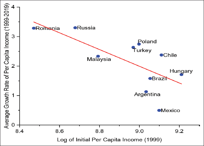
Figure 2 shows that the average growth rate of EMEs such as Romania and Russia having a low base year income are growing at a faster rate of more than 3%, whereas the growth rate of Mexico having higher base year income is growing at a rate of less than 1% during this period. EMEs such as Argentina Brazil and Hungary also show a growth rate of less than 2% during this period.

Unconditional Convergence of Below Average Income Group of EMEs

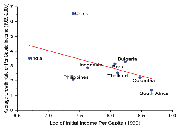
The unconditional convergence among below average income group of EMEs can be seen in Figure 3. Where China is growing at the highest rate of more than 6% and South Africa is growing at the lowest rate of less than 2% during this period.

Figure 3.

Source: World Development Indicators (2020a).

EMEs such as India, Bulgaria, and Peru are growing at a relatively higher growth rate of more than 3% than the growth rate of Colombia, Philippines, and Thailand.

Table 1.

Absolute β Convergence Results.

Groups	Periods	Constant	b (p)	R ²	N
Whole group	1999–2019	11.36342	−1.041(0.00)	0.34	19
Above average group	1999–2019	27.52169	−2.836 (0.02)	0.49	19
Below average group	1999–2019	12.08282	−1.148 (0.18)	0.23	19

Source: The authors.

Note: Figures in parentheses denote 5% level of significance.

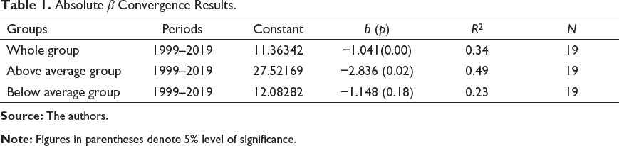
The regression results of absolute convergence are shown in Table 1, where the slope coefficient values are of negative sign for the whole group and the two subgroups of EMEs. The probability value p is low for the whole group and for the above average group of countries rejecting the null hypothesis of b = 0 But the high p value for the below average group of EMEs shows that our finding is statistically insignificant and does not reject the null hypothesis of b = 0, defying the presence of convergence in this group of EMEs. The value of R² is good for the whole and above average group of countries but is poor for the below average group of countries. Therefore, we can conclude that there is a sign of absolute convergence in EMEs for the whole and above average group of EMEs. But the below average group of EMEs do not have statistically significant results with the high p value and a low value of R². It is therefore concluded that the growth rate of below average group of EMEs is not higher to catch up to the income level of high income EMEs during the period of 1999–2019.

Conditional Convergence Results

The conditional convergence shows that countries are converging to their own levels of a steady state. The panel data regression model has been used for the conditional convergence with the controlled variables such as LFPR, EI, and GFCF. For the panel data regression, three sets of the panel have been constructed for the whole group of EMEs and the two subgroups of above average and below average group of EMEs for the period 1999–2019.

In the first set of the panel, the average annual growth rate of per capita income for the period 1999–2019 have been regressed on the base year income of 1999 and other explanatory variables. With 19 cross-sectional units and 21-time series units, a total of 399 observations are available. This data is long panel where time series units are higher than the cross-section units. The literature shows that for the long panel fixed effect model is more suitable. It can be seen from Table 2 that for the period of 1999–2019, coefficient of base year income is of the expected sign. EI, LFPR, and GFCF are also of expected sign but the regression results show that the coefficient of base year income, EI are not statistically significant at 5% level of significance. In contrast, the probability value of LFPR and GFCF is low, making the coefficient statistically significant. With a 0.63 value of R² it can be seen that there is a no conditional convergence in EMEs for the period of 1999–2019 and economies are not converging to their own steady state. But GFCF and LFPR has a significant role to play in the growth rate of EMEs.

Table 2.

Conditional Convergence Results from Fixed Effect Model (1999–2019).

Period	1999–2019
Constant	−0.437593
Base year income	−0.31113 (0.18)
Education index	2.013734 (0.17)
Labor force participation rate	0.048031 (0.00)^a
Gross fixed capital formation	0.037895 (0.07)^b
R ²	0.63
N	399
F* Test	(0.00)
Hausman test	267.03 (0.00)

Source: The authors.

Note: Figures in parenthesis are p values at ^a5% and ^b10% level of significance

*represents 5% level of significance.

Table 3 shows the second set of data where the average annual growth rate of per capita GDP of above average group of countries for the period 1999–2019 has been regressed on the base year income of 1999 and other explanatory variables.

Table 3.

Conditional Convergence Results Fixed Effect Model (2000–2008).

Period	1999–2019
Constant	40.239
Base year income	−3.455 (0.00)
Education index	2.424 (0.19)
Labor force participation rate	0.088 (0.01)
Gross fixed capital formation	0.170 (0.00)
R ²	0.58
N	210
F* Test	(0.000)
Hausman test	67.06 (0.00)

Source: The authors.

Note: Figures in parenthesis are p values. *represents 5% level of significance.

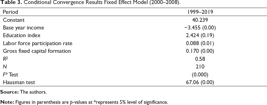
This panel includes a total of 210 observations with 10 cross sections and 21 time series units. In the above average group of EMEs, coefficient values of base year income and LFPR are negative and coefficient values of GFCF and EI are positive. The results suggest that the base year income, LFPR, and GFCF are statistically significant whereas the education index is not statistically significant. This shows that education has no role to play in the convergence of this group of EMEs. Whereas, GFCF plays a positive and significant role in the convergence process of these EMEs. Therefore, with a high value of R² and significant value of base year income, there is conditional convergence in above average group of EMEs, where GFCF and LFPR play a positive role in the growth rate of EMEs during this period.

The results of the third set of the panel where the average annual growth rate of per capita income of below average group of countries for the period of 1999–2019 has been regressed on the base year income of 1999 and other explanatory variables are presented in Table 4. Total numbers of 189 observations with 9 cross sections and 21 time series units are taken.

In the below average group of countries, coefficient values of all the controlled variables are statistically insignificant except LFPR and GFCF. With a high value of R², it can be said that the conditional variables included in the analysis do explain much of the variation in the growth rate. And there is no conditional convergence in the below average group of EMEs.

Table 4.

Conditional Convergence Results Fixed Effect Model (2008–2018).

Period	2008–2018
Constant	0.481181
Base year income	−0.62 (0.13)
Education index	0.66 (0.78)
Labor force participation rate	−0.08 (0.00)^a
Gross fixed capital formation	0.02 (0.08)^b
R ²	0.74
N	189
F* Test	(0.000)
Hausman test	242.85 (0.00)

Source: The authors.

Note: Figures in parenthesis are p values at ^a5% and ^b10% level of significance.

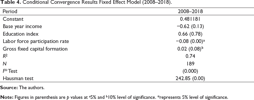
*represents 5% level of significance.

The analysis, as mentioned above, proves that there is unconditional convergence for the whole group and above average group of EMEs for the period of 1999–2019. However, there is no unconditional convergence within below average group of EMEs for the period of 1999–2019. The results on conditional convergence suggest that there is no conditional convergence within whole and below average group of EMEs but above average group of EMEs is converging conditionally. The analysis also indicates that the controlled variable such as education index has no role to play in the convergence of EMEs but the LFPR and GFCF play a significant role in the growth process of EMEs.

Unit Root Test with Structural Break

The global financial crisis which originated in the United States in 2008 was not limited to the United States only but had its impact on the other countries’ economic growth, and EMEs were no exception (McManus et al., 2014). The economic boom of EMEs post 1999 faced a slight disruption during the global financial crisis (Reddy et al., 2014). To find whether the global financial crisis had its impact on the convergence process of these EMEs, ADF unit root test with one structural break in the intercept has been performed on the relative income series of EMEs. The null hypothesis under the test statistic is of unit root in the series. The acceptance of the null hypothesis implies that the shocks to the series are permanent; hence, there is divergence of the series. Table 5 gives the descriptive statistics of relative GDP per capita of EMEs.

Table 5.

Descriptive Statistics of GDP Per Capita as a Fraction of Highest GDP Among EMEs.

Series	Observations	Mean	Std. Dev.	Minimum	Maximum	Skewness
Argentina	21	−0.35	0.10	−0.51	−0.18	−0.14
Brazil	21	−0.25	0.08	−0.41	−0.15	−0.43
Bulgaria	21	−0.77	0.13	−0.97	−0.64	−0.56
Chile	21	−0.08	0.06	−0.17	0.00	0.02
China	21	−1.24	0.39	−1.81	−0.76	−0.18
Colombia	21	−0.01	0.02	−0.06	0.00	−2.02
Hungary	21	−0.77	0.08	−0.89	−0.67	−0.25
Indonesia	21	−1.50	0.12	−1.65	−1.34	−0.01
India	21	−2.35	0.19	−2.58	−2.07	0.16
Malaysia	21	−0.33	0.09	−0.47	−0.11	1.20
Mexico	21	−0.40	0.07	−0.51	−0.30	0.01
Peru	21	−1.05	0.15	−1.25	−0.88	−0.17
Philippines	21	−1.85	0.10	−1.99	−1.70	0.09
Poland	21	−0.13	0.11	−0.28	0.00	−0.18
Romania	21	−0.54	0.14	−0.76	−0.36	−0.38
Russia	21	−0.32	0.11	−0.53	−0.19	−0.47
South Africa	21	−1.03	0.07	−1.12	−0.94	−0.11
Thailand	21	−0.21	0.11	−0.36	−0.06	0.00
Turkey	21	−0.64	0.06	−0.81	−0.55	−0.93

Source: The authors.

Note: GDP per capita as a fraction of highest GDP among EMEs = GDP per capita of EME/highest GDP among EMEs for the sample period (1999–2019) for EMEs.

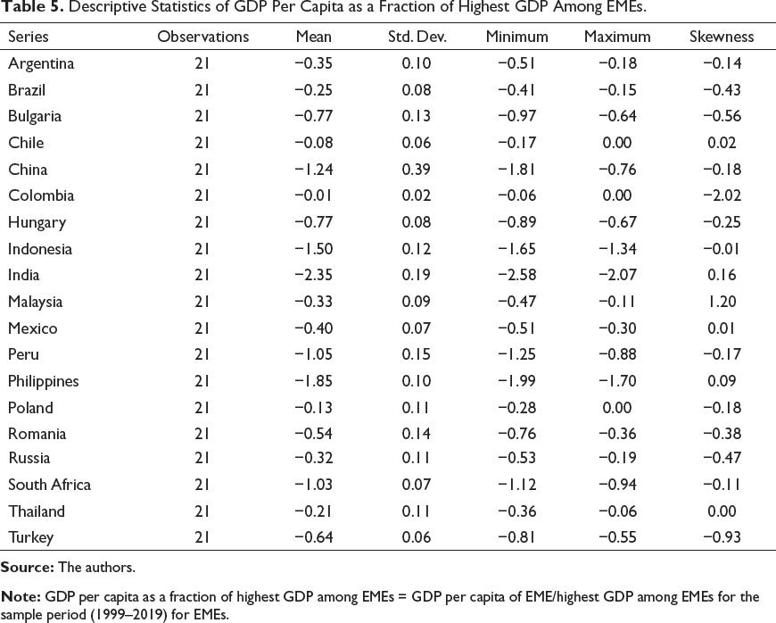
The relative series of GDP of EMEs is negative suggesting lower per capita GDP than the highest one. The positive skewness of Chile, India, Malaysia, Mexico, and Thailand suggests higher relative per capita GDP in future than the mean value.

Table 6 shows the test results of unit root test with structural break. The table shows that Chile, Colombia, Poland, South Africa, India, Indonesia, Philippines, and Thailand had structural break in the year 2008. But Argentina and Turkey had structural break in the year 2009. The reason behind this might be that the impact in these EMEs was felt in the next year.

Table 6.

Results of the ADF Unit Root Test with Structural Break.

Country	t-statistic	Estimated Break Point	B (t)	D (t)
Argentina	−3.27 (0.81)	2009	1.67 (0.13)	−1.77 (0.12)
Brazil	−2.98 (0.91)	2005	−0.71 (0.48)	0.44 (0.66)
Bulgaria	−3.82 (0.48)	2006	3.56 (0.00)	−2.41 (0.03)
Chile	−3.99(0.37)	2008	0.19 (0.84)	−2.31 (0.06)
Colombia	−3.52 (0.67)	2008	2.41 (0.02)	−1.59 (0.13)
Mexico	−4.18 (0.26)	2018	4.59 (0.00)	−5.47 (0.00)
Peru	−4.44 (0.15)^b	2007	5.25 (0.00)	−1.57 (0.13)
Poland	−5.06 (0.02)^b	2008	3.81 (0.00)	−3.15 (0.00)
Romania	−3.45 (0.71)	2006	3.40 (0.00)	−1.74 (0.10)
Russia	−3.36 (0.76)	2012	0.03 (0.97)	1.74 (0.11)
South Africa	−3.04 (0.89)	2008	2.17 (0.04)	−1.24 (0.23)
Turkey	−3.65 (0.59)	2009	2.08 (0.05)	−1.65 (0.11)
Hungary	−17.46 (0.01)	2011	−11.71 (0.00)	10.72 (0.00)
India	−3.37 (0.76)	2008	3.13 (0.00)	−2.43 (0.02)
China	−2.76 (0.95)	2013	3.82 (0.00)	−2.65 (0.02)
Indonesia	−5.50 (0.01)^a	2008	6.22 (0.00)	−3.23 (0.00)
Philippines	−4.23 (0.24)	2008	2.93 (0.01)	−1.83 (0.08)
Malaysia	−3.45 (0.71)	2014	−0.41 (0.68)	1.88 (0.08)
Thailand	−4.64 (0.08)^c	2008	4.41 (0.00)	−3.31 (0.00)

Source: The authors.

Note: The critical values for each test are:

Test critical values:	1% level	−5.3476
	5% level	−4.85981
	10% level	−4.60732

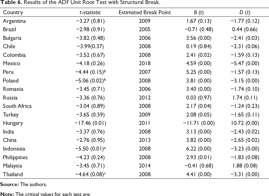
^a, ^b, and ^c denotes statistical significance at 1%, 5%, and 10% level of significance.

The null hypothesis of unit root in the series cannot be rejected for the EMEs except Poland, Hungary, Indonesia, and Thailand. These EMEs have the test value less than the critical value. The presence of unit root shows that shocks to the series are permanent and there will be divergence of the series. Whereas rejection of the hypothesis implies that the shocks to the series will be temporary and there will be convergence of the series. Based on the test results only Poland, Hungary, Indonesia, and Thailand show convergence in the GDP per capita during the sample period. The significance of the dummy variables show that only Chile, India, Poland, Philippines, and Thailand has significant impact of the financial break on the relative income series of these EMEs.

“σ” Convergence Results

The graphical view of the σ convergence shows the trend of CV of log per capita income and other explanatory variables such as LFPR, EI, and GFCF. Figure 4 shows the declining CV of log per capita GDP for the whole sample and for both the subgroups. The year of 2019 draws a different pattern for these EMEs. The CV for whole and below average group is increasing showing the divergence whereas the CV for above average group is declining showing convergence in that year. The possible explanation for this behavior can be the impact of COVID-19 at the end of the year. Since China having the largest share among below average income EMEs and the initial impact was felt on China there is divergence in EMEs. However, the impact of COVID-19 was not widespread to other countries till the start of 2020. Therefore, there is increasing convergence among above average EMEs.

Figure 4.

Source: World Development Indicators (2020a).

Figure 5.

Source: Human Development Reports (2020).

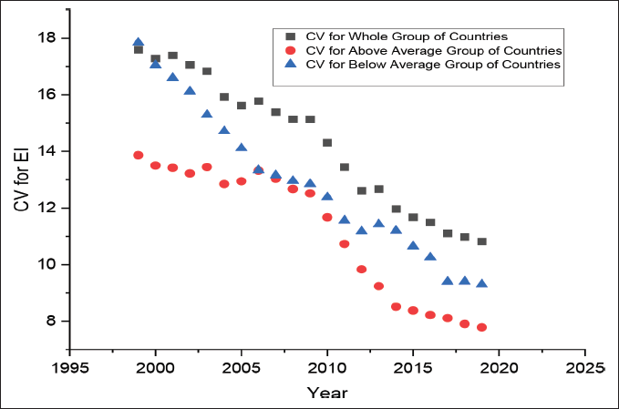
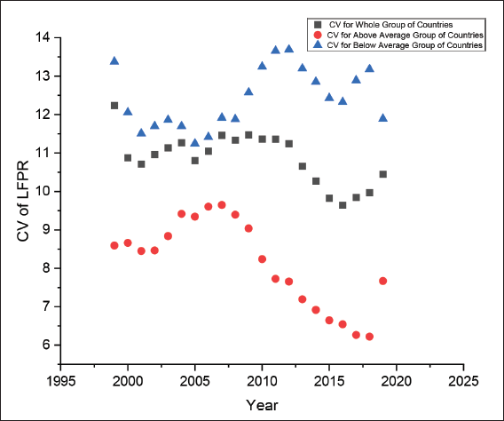
Figure 5 shows the declining trend of CV of education index for the three groups of countries showing σ convergence. This shows that the variations in the EI for all three groups were declining. This can happen either with the declining level of education of above average group or with the increasing education level of below average group. Even within both the subgroups, the disparity was declining. The graphical presentation of CV for LFPR in Figure 6 shows a different pattern. The whole group shows convergence of LFPR after 2011 but the pattern changed after 2016 with divergence in the data. The variability of LFPR within above average group increased till 2008 but started declining after that and showed a sudden increase in 2019. The below average group of EMEs shows a wavy pattern in Figure 6, where convergence in LFPR shows a sudden decline in the year 2019 after the increase in 2016.

Among the group B EMEs, Peru had the highest number of workforce participation rate of 77% in the year 2018. Other countries with higher workforce participation rate, including China, Colombia, and Thailand with 68%, 68%, and 67% share, respectively, also belonged to below average group. Whereas India and Turkey had the lowest rate of labor force participation with a percentage of 49 and 52, respectively. Above average EMEs such as Argentina, Brazil, Poland, and Russia and below average EMEs such as Colombia, South Africa, and Indonesia maintained a more or less stable LFPR during 2000–2018. Peru has faced the largest change during this period with a 10% increase in its LFPR from 67% in 2000 to 77% in 2018. Other EMEs which have shown relatively higher changes during this period are Romania, China, and India, but the difference in these EMEs indicate a decline of 9%, 9%, and 8%, respectively (World Development Indicators, 2020a). This decline of LFPR shows the increase in joblessness in these EMEs during this period.

Figure 6.

Source: World Development Indicators (2020a).

Figure 7.

Source: World Development Indicators (2020c).

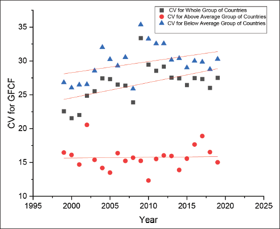
The increasing trend line in Figure 7 shows that the variation within EMEs as a group of whole and within below average group was increasing during the entire period. Thus, there is a σ divergence of GFCF within EMEs. The trend line of group A countries shows that the variation in GFCF during this period remains more or less stable with short-term slight fluctuations. The reasons for such a trend can be understood with the description of some EMEs below.

Latin American EMEs such as Argentina, Brazil, Chile, Peru, and Mexico had an investment boom during 2003–2008 with a real investment growth rate of 10% (Izquierdo et al., 2008). The investment growth was accompanied by the rise in international commodity prices. However, after the financial crisis from 2009 to 2016, the growth in investment slowed down to 0.94%. The momentum in investment became slow after 2011 due to declining global growth, rising uncertainty in the domestic market, and tighter financial conditions. In the case of Colombia, investment was consistently increasing after 2000 and remained more or less stable even after the crisis within the range of 28%–29%. Both the economic growth and aggregate demand has played an important role in the rising investment of Colombia (CEPAL, 2018).

Central and Eastern European (CEE) countries Bulgaria, Romania, Hungary, and Poland reached its peak of 36%, 33%, 25%, and 24%, respectively, during 2008–2009 but was on a declining spree after the crisis. Investment in these countries was related to the GDP growth, which has shown a similar trend of upturn before the crisis and of a downturn after the crisis.

India had the second largest capital formation among EMEs after China until 2014. GFCF in India reached its peak of 41% in 2008, flattered by its economic growth during this period. With declining GDP growth after 2011 due to unfavorable external conditions, pervasive corruption charges against the government and rising nonperforming assets in the bank’s balance sheets dissuaded the private sector from undertaking any investment. Moreover, the limited fiscal space of the government restrained public sector investment.

Investment in China is mainly state driven. There is a direct influence of the Chinese government in the investment decisions of the economy either by investing in large projects or by affecting the interest rates and tax rates. As a result, China has seen a sustained rise in its GFCF after 2001 and a substantial rise after the global financial crisis. There has been a declining trend in investment after 2011, showing the slowdown in the economy but still maintaining the highest share among EMEs.

In South Africa, the growth rate of real gross fixed capital formation from 2000 to 2008 was around 9%, which decelerated to 0.6% after the crisis. Weak export demand for South African commodities, declining investor’s confidence due to weak output growth in the mining sector and labor strikes caused a decline in the capital formation by an average of 20% in South Africa after the crisis.

Growth Trend of Selected EMEs During the Period (1999–2019)

Argentina

Argentina had erratic economic growth since 1995 due to external economic shocks, higher debt, and volatile capital flows. This was followed by the sharpest decline of GDP in the year 2001–2002. Expansionary fiscal policies and re-nationalization of public utilities were undertaken to revive the economy. These measures doubled the size of the economy from 2002 to 2011 (Hornbeck, 2013). The growth rate was averaged around 9% for the period 2003 to 2007. The global financial crisis of 2008 affected the Argentine economy with a decline of GDP by 6% in the year 2009. But this decline lasted for a very short period of time and economy rebounded in 2010 with a 10% growth rate. Downturns in trading partners, increasing inflation and austerity measures by the government reduced the growth rate of the economy from 2012 with a slight revival in 2015. But higher inflation and depreciating currency reduced the growth rate to −2% in 2018. Figure 5 shows the inflation trend in Argentina from 2000 to 2018. It led IMF to provide the largest financial support ever of $57 billion to Argentina in 2018 (Nelson, 2020). Measures such as deferring of the debt payment, postponement of repayment to IMF, and restrictions on capital flights were taken to avoid the crisis and help revive the economy.

Brazil

With the beginning of this century, the Brazilian economy faced serious problems of inflation, rising unemployment, and political uncertainties. In the mid of 2004, this trend reversed, and the Brazilian economy started making social and economic progress. The period of 2003 to 2014 was the period of boom where Brazil lifted 30 million people out of poverty (The World Bank, 2020) and Gini coefficient, measuring inequality, declined significantly. The significant contraction in economic activity from 2014 was the result of falling commodity prices and the country’s inability to introduce fiscal reforms (Rugitsky, 2017). For reviving the economic growth of the nation, many fiscal reforms including the constitutional amendment of 2016 to limit public spending and to stabilize the public debt at a sustained level were enacted by the government (Brescianini, 2018). As a result of these measures, economic activity revived in the year 2017 with the 1.1% growth rate of GDP. Nevertheless, the weak labor market, trucker’s general strike and uncertainties looming around general elections brought a break in the revival of the economy.

Bulgaria

Sound financial policies, privatization, and the introduction of currency board regime by the government in the year 1997 helped the economy to take off from 2003, and this trajectory continued till 2007 when Bulgaria joined the European Union. The global financial crisis hit the economy in the last quarter of 2008. With the disruption in the gas supplies in the Russian Ukraine dispute, the Bulgarian economy faced a difficult start in 2009. The economy declined by 5% in 2009. This contraction in GDP continued in 2010 with a 4% decline in the GDP. Rising export demand, better harvest, and weak domestic demand helped to revive the growth in 2011 (Overview: Countries Compared, 2013). The economic growth remained weak to less than 2% until 2014. However, with rising export demand, the inflow of EU development funds accompanied by declining international energy prices in the coming years, helped to boost the economic growth of Bulgaria after 2014.

Chile

After the decline of 1998–1999, the growth rate of Chile recovered in 2000 caused by the strong world economic growth. The average growth rate from 2000 to 2008 remained at 5% per annum. This growth trajectory was halted with a decline of GDP by 1.5% in 2009 because of global financial crisis. Growth revived in 2010 with a GDP growth of 5.8% as a result of increase in trade surplus and a decrease in public debt (World Development Indicators, 2020b). In 2013, the decline in copper prices and lower international prices of other exportable commodities decreased the trade surplus and weakened the economic growth.

Colombia

After the reforms of 1990 Colombian economy started showing an upward trend and gradually became integrated with the world economic system. The rising prices of oil and other minerals, increasing state spending, access to international financial market at a cheaper cost and increasing remittances from the United States and Spain helped in the economic growth during this period. The economic boom from 1999 to 2007 was interrupted by the global financial crisis (Ocampo, 2015). GDP growth declined to 3.2% and 1.4% in the year 2008 and 2009, respectively. With the favorable external conditions, economy grew with an average annual growth rate of 5.3% from 2011 to 2013. But after 2013 domestic inequality and slowdown in world economy adversely affected the Colombian economy. In recent years declining oil prices and increasing attacks on pipelines are the major factors for the slowdown of growth to 1.4% in 2017 (World Development Indicators, 2020b). Following this slowdown, the economy saw revival in 2019 as a result of increasing consumption and investment; however, with the outbreak of pandemic, the growth rate has been halted.

Mexico

After the crisis of 1994, administrative reforms improved the growth rate in Mexico. Following these reforms, Mexican economy faced a period of brief stagnation during 2001 and recovered with an average growth rate of 3.5% during 2004–2006. It helped the Mexican economy to enter the trillion-dollar club in 2005 and became the biggest economy in Latin America (Ocampo, 2009). The global financial crisis of 2008 affected the Mexican economy with a contraction of around 5% in its GDP. The reason being that Mexican economy was heavily dependent on its exports to the United States, which was the center of this crisis. Following the crisis, Mexican economy started recovering after 2010 with the increase of its exports. The Mexican economy has shown great resilience in the past few years with reduction in the inflation rate and increase in its per capita income. However, specific unresolved issues such as lower wages, regional inequality between north and south and lower tax to GDP ratio has kept the growth rate within the range of 2%–3% from 2014 to 2019 (Mexico Economy, 2020).

Peru

Dependence of the Peruvian economy on exports benefited it with the rising international commodity prices during 2001–2008. The Peruvian economy was growing at 9.1% in 2008 but with the eruption of global financial crisis, GDP growth reduced in 2009 to 1% with the inflation rate nearly zero. However, with the adoption of countercyclical policies the growth revived to 8% in 2010. In 2013 with the onset of the global slowdown Peru suffered a decline in its GDP growth. The growth rate remained at around 3% during 2014–2018. Weaker external demand, lower private investment, and declining commodity prices were some of the factors responsible for this decline.

Poland

Reforms in Poland after the fall of communist era yielded an average growth rate of 5% from 1999 to 2007. However, this growth rate was lower than the other former communist economies because of the large budget deficit, tighter monetary policy and lack of second-generation reforms after the fall of the communist set up. With the outbreak of the global financial crisis, entire Europe suffered from recession. Poland was the only nation to avoid a crisis in Europe (Pleitgen & Davies, 2010) and grew at a rate of 2.8% in 2009. The growth rate of Poland was highest during 2010 and 2011 at an average of 4% among all EU nations. After the crisis, the GDP of the EU declined as a whole but the GDP of Poland increased by 20% between 2008 and 2012. The reasons for this phenomenal growth were the countercyclical policies and strong macroeconomic fundamentals adopted during 2000–2007. However, the growth rate started slowing down after 2011 because of a decline in the rate of investment and private consumption. The economy grew from 2013 to 2015 at an average rate of 3% but slowed down after 2016 as a result of the tighter labor market and declining industrial output.

Romania

The transition to free market in Romania started with its new constitution in 1991, which was followed by its membership in NATO in 2004 and EU membership in 2008. This predominantly drove the economic growth in Romania from 2000 to 2007. Foreign investment, trade with EU, and domestic investment also played an important part in the growth process. In its pursuance to join the EU, Romania adopted many policy reforms in 2005, including a flat tax rate of 16% and privatization of state bank. Romania’s accession to the EU in 2007 further opened its growth potential. However, during the global financial crisis in 2008 the economy of Romania was affected adversely and shrank in 2009 (FleŞer & Criveanu, 2012). Even after receiving an assistance package of US$25.5 billion from international organizations such as the EU and IMF, its GDP contracted further in 2011. The economy revived in 2013 and continued its growth trajectory until 2017 with an increase in industrial exports and expansionary policies. Exports into the EU, domestic demand, and tax cuts helped to boost the economy during this period. Recently growth has slowed down because of the reduction in the fiscal stimulus package, massive corruption scandals, and ageing of the population.

Russia

Russia had negative growth rate in the last decade of the twentieth century barring a few months in 1998. After facing the financial crisis of 1998 due to the collapse of oil prices Russia achieved macroeconomic stability during 2000–2008 with the help of fiscal discipline and a continuous budget surplus since 2000. Rising commodity prices in the international market gave a significant boost to economic growth during 2000–2007. The global financial crisis hit the Russian economy in mid-2008 and the growth rate declined to −7.8% in 2009 (World Development Indicators, 2020b). But with the strong macroeconomic fundamentals, Russia was able to wither away its effects and started recovering from 2010 onward. With the global slowdown in 2013, oil prices declined, hitting the Russian economy hard as 70% of its revenues came from oil and natural gas in 2012 (Country Analysis Brief: Russia, 2017). Russia again faced a financial crisis in 2014. The annexation of Crimea and conflict in Ukraine led the United States, European Union, Canada, and Japan to impose sanctions on Russia. It reduced the growth rate to 0.7% in 2014. Russian economy entered into a recession with a 4.5% contraction of its GDP in 2015. However, in 2016 Russia came out of recession with a positive growth rate of 0.19% and continued to grow in 2017 at 1.8%. More recently, Russia has grown at a positive but a low rate of growth till 2019.

Turkey

The economic growth of Turkey declined to 4% per annum during 2007–2014 from an average of 6.1% during the economic boom of 2002–2007. The growth rate was at its lowest at 0.8% in 2008 with a sharp contraction of GDP by 4.6% in 2009 (World Development Indicators, 2020b). After the crisis, reduction of interest rate to almost zero, increasing government spending, and a primary surplus of state-owned enterprises played a significant role in reviving the economic growth. The growth rate remained at around 9% in 2010 and 2011. However, this growth was marked as a low-quality growth. It was triggered by the increasing foreign currency debt of companies from the outside investors and rising imports than exports that caused higher current account deficit. The declining value of the lira against the dollar made payment of foreign debt difficult putting companies at risk of default. Thus, the declining value of the lira, high inflation, and rising risk of default pushed the Turkish economy into recession in recent years (The World Bank, 2020).

Hungary

Measures taken during the 1990s helped Hungary to grow at a historically high growth rate in 2000s decade. Following these reforms, Hungary joined European Union in 2004. This growth from 2001 to 2008 was led by the increasing exports and rising commodity prices in the international market. Falling demand for exports, declining agricultural output and slump in the construction sector as a result of financial crisis in 2008 contracted the economy by 5% in 2009. But with the rising export demand, especially from Germany helped the economy to revive in 2010 with an economic growth of 1.5% in 2011. However, economy faced a minor recession in 2012 but with the utilization of EU funds and subsidized loans to micro small and medium enterprises (MSMEs) helped the growth to pick up in 2014 and 2015. Reduction in taxes by the government increased the domestic demand, which helped in the revival of the economy in 2018 and 2019. However, challenges of corruption, decline in demography, migration, and heavy reliance on export demand are some of the vulnerabilities of faced by the Hungarian economy (Hungary Economy, 2020).

China

China had shown consistent growth rate of more than 6% per annum after the market reforms of 1978 (World Development Indicators, 2020b). After joining the world trade organization in 2000, China’s export-led growth model helped to achieve an average growth rate of 10.2% per annum from 2000 to 2010. During this decade China became the world’s largest manufacturer, trader, and holder of foreign exchange reserves. China’s trade in 2006 surpassed the 1.75 trillion dollar mark, and it became the largest trading nation in the world. It helped China to achieve a growth rate of 14.2% in the year 2007, highest since 14.2 of 1994 (Morrison, 2019). Due to the financial crisis of 2008 the growth rate slowed down to less than 9.6% in 2008. Chinese economic growth model was an export-oriented model and the fall in global economy affected the growth of Chinese economy. However, from 2010 onward, China’s growth started slowing down due to the slowdown in the global economy and the maturity of the Chinese growth model. Even after this slow down, the growth rate remained highest in the world (Morrison, 2019).

India

Liberalization, privatization, and globalization (LPG) reforms of 1991 in India started yielding fruits with the beginning of the twenty-first century. The decade of 2000s was the golden period of economic growth in India since its independence. From 2004 to 2008, it was the second fastest growing economy in the world after China, with an annual average growth rate of 7%. This story of growth faced a slight disruption in the year 2008 due to the global financial crisis but recovered soon as the Indian banking sector was not much exposed to international finances. The growth rate slowed down in the first quarter of the year 2011. Global slowdown, pervasive corruption charges against the government and declining investors’ confidence contributed to this slowdown. The growth revived in 2014 but again started slowing down from 2016 onward (Laborde & Martin, 2016). This slow down attributed to declining credit supply because of rising nonperforming assets in the balance sheets of banks and structural changes such as tax reforms and demonetization of high denomination currency. All this contributed to the decline of investment and hindered the growth rate of the Indian economy.

Indonesia

The Indonesian economy exhibited a steady growth after facing the Asian financial crisis of 1997 (Asian Financial Crisis in Indonesia, 2020). Increasing domestic consumption has contributed to a growth rate of 5% in 2004 and 2005. The growth rate rose to 6.5% in 2007 at its 10 years high level. Domestic demand and a fiscal stimulus package helped the economy to shrug away the impact of the crisis (Basri & Rahardja, 2010) making it one of the third fastest growing economies in Asia after China and India in 2010. Indonesian economy faced a slowdown from 2011 to 2015 with an average growth rate of 5.5%. The economy revived slightly during 2016. However, due to decreasing trade, depreciation of Indonesian currency and declining consumer spending, growth rate further slowed down after 2017 (Salna & Rahadiana, 2018).

Malaysia

After the Asian financial crisis, economic stimulus package helped the Malaysian economy to grow at an average growth rate of 5.5% in the first decade of twenty-first century. The economy transformed itself into a manufacturing hub and became a leading exporter of electronic components. Increasing labor productivity, rising export demand, and increasing manufacturing activities helped the economy to grow steadily till 2008. The global slowdown of 2008 contracted the economy by 1.5% in 2009 but with a strong recovery, growth rate rose to more than 7% in 2010. The average growth rate remained 5% from 2011 to 2015. Rising domestic demand and increasing export of oil and gas were the main drivers of economic growth during this period. However, weak international commodity prices and depreciating ringgit reduced the current account surplus during 2013–2017, which put a strain on the government revenues. The economy showed a steady recovery from 2017 onward but the recent crisis of COVID pandemic has slowed down the economic activities.

Philippines

In the Philippines, growing remittances from overseas Filipino workers and the growing business processing outsourcing industry played an important role in its growth after the Asian financial crisis of 1997. In 2010, remittances were 10% of its GDP surpassing the foreign direct investment as a source of foreign currency. Its GDP grew at an average of 4.5% between 2001 and 2009 and the Philippines began to categorize as a newly industrialized economy. After a short decline of growth in 2009 to 4.6% the Philippines grew at a rate of 6.2% in 2010. The inadequate infrastructure spending and declining exports and imports reduced the growth rate after 2010. However, increasing domestic demand, substantial remittances and vital labor market helped the Philippines to become the third largest growing economy in 2013 after China and India with a growth rate of 5.5%. The reasons behind the sustained economic growth of 6%–5% from 2011 to 2019 were its dynamic manufacturing sector, competitive workforce, and strong macroeconomic fundamentals, which played an important role (Bajpai, 2020).

Thailand

After the financial crisis of 1997, Thailand’s economy faced contraction of 10.5% in its GDP. Growth revived in 1999 and reached to the pre-crisis level in the year 2002. Thailand paid its IMF debt in 2003, but at the end of year 2004, tsunami in Indian Ocean affected the GDP growth in 2005. GDP growth declined from 6.3% in 2004 to 5.1% in 2005. Military coup in 2006, global financial crisis in 2008, floods in 2010 and 2011, and Eurozone crisis in 2012 kept the growth rate very low from 2007 to 2012. Thailand faced a negative growth rate of −2.3% in 2009 for the first time after the financial crisis of 1997. Political turmoil reduced the private consumption and investor’s sentiment and the decline of exports due to the Eurozone crisis were the major reasons for this decline. The average annual growth rate remained at 3.25% from 2007 to 2012. Thai economy suffered from recession from 2014 to 2017. Poverty rate and inequality increased during this period. In 2018, economy showed best results since 2014 but declined in 2019 due to the global slowdown and rising trade war between the United States and China. With the outbreak of COVID-19 pandemic the economy is expected to further contract in 2020.

Conclusion and Implications

This study aims to find the convergence of per capita income in the EMEs. Methods of σ and β convergence have been used to check if EMEs are converging toward a common level of per capita income or not. For the unconditional β convergence, a cross-sectional analysis was conducted. Additionally, for the conditional convergence, panel data regression was performed. To check whether global financial crisis had its impact on the convergence process of EMEs, unit root test with one structural break has been performed. The results of the study prove that there is unconditional convergence in EMEs for the period 1999–2019 for the whole group and the above average group of EMEs. However, there is an absence of unconditional convergence in the below average group of EMEs. The controlled variables under panel data regression are GFCF, EI, and LFPR. The regression results for panel data show that there is no conditional convergence in the whole and below average group of EMEs, but significant values of GFCF and LFPR indicate their important role in the average growth rate of these EMEs. However, the high-income EMEs or the above average group has conditional convergence for the period 1999–2019, where LFPR and GFCF has significant role to play in their convergence process.

The significant values of dummy variables in the unit root test with structural break for Poland, India, Philippines, and Thailand show that the financial crisis had significant impact on the relative income series of EMEs. Finally, the results of σ convergence show that EMEs are converging in σ sense as the difference in the per capita income level of EMEs is declining over time, showing a clear sign of convergence in EMEs for the sample period.

Some of the implications of the study are:

The results indicate that there is no unconditional and conditional convergence in the low-income EMEs as their growth rate is smaller than high-income EMEs.

The controlled variables such as gross fixed capital formation and labor force participation has significant role to play in the growth of EMEs. Therefore, attention should be paid on these factors for the low income EMEs to catch up with the income level of high income EMEs.

Limitations of the Study

Various factors affect the conditional convergence of economies such as saving rate, labor force participation rate, inflation rate, education and health infrastructure, gross fixed capital formation, financial inclusion, R&D expenditure, and trade of goods and services. This study includes only gross fixed capital formation, education, and labor force participation rate as a proxy for human and physical capital for a brief analysis. Hence, there is further scope for detailed analysis by considering all the variables and their effects on the convergence process of EMEs.

Footnotes

Acknowledgments

The authors are grateful to the anonymous reviewers of the journal for their valuable comments in improving the quality of this article.

Declaration of Conflicting Interests

The authors declare no conflict of interest with respect to research, authorship, and publication of interest of this articles.

Funding

The authors received no financial support for the research, authorship, and publication of this article.

Notes

References

Anoruo

(2019). Testing for convergence in per capita income within ECOWAS. Economia Internazionale/International Economics , 72(4), 493–512.

Asian Financial Crisis in Indonesia. (2020). Asian financial crisis in Indonesia . https://www.indonesia-investments.com/culture/economy/asian-financial-crisis/item246

Bajpai

(2020, May 4). Emerging markets: Analyzing the Philippines’s GDP . https://www.investopedia.com/articles/investing/091815/emerging-markets-analyzing-philippines-gdp.asp

Barro

R. J.

, & Sala-i-Martin

(1992). Convergence. Journal of Political Economy , 100(2), 223–251.

Barro

R. J.

, Sala-i-Martin

, Blanchard

O. J.

, & Hall

R. E.

(1991). Convergence across states and regions. Brookings Papers on Economic Activity , 1, 107–182.

Basel

, & Rao

R. P.

(2018). β Convergence of real per capita GDP in BRICS economies. Indian Journal of Economics Development , 14(2), 309–315.

Basri

M. C.

, & Rahardja

(2010). The Indonesian economy amidst the global crisis: Good policy and good luck. ASEAN Economic Bulletin , 27(1), 77–97.

Baumol

(1986). Productivity growth, convergence, and welfare: What the long-run data show. The American Economic Review , 76(5), 1072–1085.

Beenstock

, & Felsenstein

(2008). Regional heterogeneity, conditional convergence and regional inequality. Regional Studies , 42(4), 475–488.

10.

Bems

M. R.

, Caselli

F. G.

, Grigoli

, Gruss

, & Lian

(2018). Is inflation domestic or global? Evidence from emerging markets (Working Paper No. 18/241). https://www.imf.org//media/Files/Publications/WP/2018/wp18241.ashx

11.

Brescianini

J. N. S.

(2018). Brazil policy note returning to a sustainable fiscal path . https://pubdocs.worldbank.org/PubDocsError.jsp?err_msg=Document%20is%20not%20available%20for%20public%20viewing

12.

Button

K. J.

, & Pentecost

(1995). Testing for convergence of the EU regional economies. Economic Inquiry , 33(4), 664–671.

13.

Çamurdan

, & Ceylan

(2013). Convergence experiences in emerging market economies (1950–2008). Journal of Yasar University , 8(30), 5105–5122.

14.

Cass

(1965). Optimum growth in an aggregative model of capital accumulation. The Review of Economic Studies , 32(3), 233–240.

15.

CEPAL

N. U.

(2018). Economic survey of Latin America and the Caribbean 2018. Evolution of investment in Latin America and the Caribbean: Stylized facts, determinants and policy challenges. Santiago: ECLAC (Economic Commission for Latin America and the Caribbean).

16.

Country Analysis Brief: Russia. (2017). Country analysis brief: Russia . https://www.eia.gov/international/analysis/country/RUS

17.

Cuaresma

J. C.

, Havettová

, & Lábaj

(2013). Income convergence prospects in Europe: Assessing the role of human capital dynamics. Economic Systems , 37(4), 493–507.

18.

Cubeddu

M. L. M.

, Culiuc

M. A.

, Fayad

M. G.

, Gao

, Kochhar

M. K.

, Kyobe

M. A. J.

, Oner

, Perrelli

, Sanya

, Tsounta

M. E.

, & Zhang

(2014). Emerging markets in transition: Growth prospects and challenges (Staff Discussion Note 14/06). International Monetary Fund.

19.

Das

R. C.

, Das

, & Das

(2019). BRICS nations and income convergence: An insight from the quarterly data for 2006Q1–2017Q2. Global Business Review , 1–16. https://doi.org/10.1177/0972150918822057

20.

Dey

S. P.

, & Neogi

(2015). Testing sigma and unconditional beta convergence of GDP for SAARC countries: Can inclusion of China further consolidate the convergence? Global Business Review , 16(5), 845–855.

21.

Dvoroková

(2014). Sigma versus beta-convergence in EU28: Do they lead to different results. Mathematical Methods in Finance Business Administration . Proceedings of the 1st WSEAS International Conference on Pure Mathematics (PUMA’14), Tenerife, Spain, pp. 88–94.

22.

Elangovan

(2019). BIMSTEC, a weak cross-border organisation? The growing economies show convergence. ПетрозаводсК (Petrozavodsk) , 26, 13.

23.

Fernandes

(2011). Global convergence of financing policies: Evidence for emerging-market firms. Journal of International Business Studies , 42(8), 1043–1059.

24.

FleŞer

, & Criveanu

R. C.

(2012). Some consequences of the economic crisis in Romania. Annals of the University of PetroŞani. Economics , 12, 135–142.

25.

Friedman

(1992). Do old fallacies ever die? Journal of Economic Literature , 30(4), 2129–2132.

26.

Ganong

, & Shoag

(2017). Why has regional income convergence in the US declined? Journal of Urban Economics , 102, 76–90.

27.

Hoen

H. W.

(2014). Globalization and institutional change: Are emerging market economies in Europe and Asia converging? Economics, Management, Financial Markets , 9(4), 44–66.

28.

Hornbeck

J. F.

(2013). Argentina’s post-crisis economic reform: Challenges for US policy . Congressional Research Service.

29.

Howitt

(2000). Endogenous growth and cross-country income differences. American Economic Review , 90(4), 829–846.

30.

Human Development Reports. (2020). Human development reports . http://hdr.undp.org/en/content/education-index

31.

Hungary Economy. (2020, January 27). Hungary economy 2020 . https://theodora.com/wfbcurrent/hungary/hungary_economy.html

32.

Islam

(1995). Growth empirics: A panel data approach. The Quarterly Journal of Economics , 110(4), 1127–1170.

33.

Ito

(2017). Growth convergence and the middle-income trap. Asian Development Review , 34(1), 1–27. https://doi.org/10.1162/ADEV_a_00079

34.

Izquierdo

, Romero-Aguilar

R. S.

, & Talvi

(2008). Booms and busts in Latin America: The role of external factors (IDB Working Paper No. 532). https://doi.org/10.2139/ssrn.1820920

35.

Jayanthakumaran

, & Lee

S. W.

(2013). Evidence on the convergence of per capita income: A comparison of founder members of the Association of South East Asian Nations and the South Asian Association of Regional Cooperation. Pacific Economic Review , 18(1), 108–121.

36.

Johnson

, & Papageorgiou

(2020). What remains of cross-country convergence? Journal of Economic Literature , 58(1), 129–175.

37.

Koopmans

(1963). On the concept of optimal economic growth . Yale University. https://EconPapers.repec.org/RePEc:cwl:cwldpp:163

38.

Korotayev

, Zinkina

, Bogevolnov

, & Malkov

(2012). Global unconditional convergence among larger economies after 1998? Journal of Globalization Studies , 2(2), 246–280.

39.

Laborde

, & Martin

W. J.

(2016). Implications of slowing growth in emerging market economies for hunger and poverty in rural areas of developing countries (Discussion Paper 01554, p. 58). IFPRI.

40.

Lenka

(2016). Per capita income convergence (or divergence) across the states of India: Post reform experience. Orissa Economic Journal , 48(1&2), 64.

41.

Martin

, & Sunley

(1998). Slow convergence? The new endogenous growth theory and regional development. Economic Geography , 74(3), 201–227.

42.

Mathur

S. K.

(2005). Economic growth & conditional convergence: Its speed for selected regions for 1961–2001. Indian Economic Review , 40(2), 185–208.

43.

McManus

, Floyd

, Abd Majid

M. S.

, & Kassim

S. H.

(2009). Impact of the 2007 US financial crisis on the emerging equity markets. International Journal of Emerging Markets , 4(4), 341–357.

44.

Mexico Economy. (2020, January 27). Mexico economy 2020 . https://www.theodora.com/wfbcurrent/mexico/mexico_economy.html

45.

Mishra

, & Mishra

(2018). Is there conditional convergence in the per capita incomes of BIMAROU states in India? Economic Modelling , 70, 429–437.

46.

Morrison

W. M.

(2019). China’s economic rise: History, trends, challenges, and implications for the United States. Current Politics Economics of Northern and Western Asia , 28(2/3), 189–242.

47.

Nahar

, & Inder

(2002). Testing convergence in economic growth for OECD countries. Applied Economics , 34(16), 2011–2022.

48.

Nelson

R. M.

(2020). Argentina’s economic crisis and default . https://crsreports.congress.gov/product/pdf/IF/IF10991

49.

Ocampo

J. A.

(2009). Latin America and the global financial crisis. Cambridge Journal of Economics , 33(4), 703–724.

50.

Ocampo

J. A.

(2015). Performance and challenges of Colombian economy. In Colombia’s political economy at the outset of the twenty-first century: From Uribe to Santos and beyond (pp. 3–33). Lexington Books.

51.

Overview: Countries Compared. (2013). Overview: Countries compared . https://www.nationmaster.com/countryinfo/stats/Economy/Economy/Overview

52.

Paas

, & Schlitte

(2006). Regional income disparities: Convergence or divergence within the EU-25 [Paper presentation]. 14th INFORUM Conference, Traunkirchen, Austria.

53.

Pleitgen

, & Davies

(2010, June 29). How Poland became only EU nation to avoid recession . http://edition.cnn.com/2010/WORLD/europe/06/29/poland.economy.recession/index.html

54.

Quah

(1993). Galton’s fallacy and tests of the convergence hypothesis. The Scandinavian Journal of Economics , 95(4), 427–443.

55.

Raiser

, Wes

, & Yilmaz

(2016). Beyond convergence: Poland and Turkey en route to high income. Central Bank Review , 16(1), 7–17.

56.

Ram

(2018). Comparison of cross-country measures of sigma-convergence in per-capita income, 1960–2010. Applied Economics Letters , 25(14), 1010–1014.

57.

Ramsey

F. P.

(1928). A mathematical theory of saving. The Economic Journal , 38(152), 543–559. https://doi.org/10.2307/2224098

58.

Reddy

K. S.

, Nangia

V. K.

, & Agrawal

(2014). The 2007–2008 global financial crisis, and cross-border mergers and acquisitions: A 26-nation exploratory study. Global Journal of Emerging Market Economies , 6(3), 257–281.

59.

Rodrik

(2011). Unconditional convergence . https://EconPapers.repec.org/RePEc:nbr:nberwo:17546

60.

Romer

P. M.

(1986). Increasing returns and long-run growth. Journal of Political Economy , 94(5), 1002–1037.

61.

Rugitsky

(2017). The rise and fall of the Brazilian economy (2004–2015): The economic antimiracle (Working Paper Series 2017_29, pp. 1–44). FEA/USP.

62.

Salna

, & Rahadiana

(2018, May 7). Indonesian GDP growth disappoints, adding to currency woes . https://www.bloomberg.com/news/articles/2018-05-07/indonesia-s-economy-expands-at-slower-pace-than-forecast

63.

Solow

R. M.

(1956). A contribution to the theory of economic growth. The Quarterly Journal of Economics , 70(1), 65–94.

64.

Sraders

(2018, February 11). What are emerging markets? Characteristics and list . https://www.thestreet.com/markets/emerging-markets/what-are-emerging-markets-14819803

65.

The World Bank. (2020, November 18). The World Bank in Brazil: Overview . https://www.worldbank.org/en/country/brazil/overview

66.

The World Bank. (2020, October 19). The World Bank in Turkey . https://www.worldbank.org/en/country/turkey/overview

67.

Tsounta

(2014). Slowdown in emerging markets: Sign of a bumpy road ahead? (IMF Working Paper). https://dx-doi-org.web.bisu.edu.cn/10.5089/9781498304719.001

68.

ur Rehman

M. A.

, & Hayat

M. A.

(2017). Capital account liberalization and economic growth evidence from emerging market economies. Pakistan Economic and Social Review , 55(1), 299–313. https://doi.org/10.2307/26730223

69.

Wooldridge

J. M.

(2016). Introductory econometrics: A modern approach (5th ed.). Nelson Education.

70.

World Development Indicators. (2020a). World development indicators . https://databank.worldbank.org/reports.aspx?source=2&series=SL.TLF.CACT.ZS&country=ARG,BRA,MEX,PER,COL,CHL,BGR,POL,ROU,HUN,TUR,ZAF,RUS,IND,IDN,CHN,MYS,PHL,THA

71.

World Development Indicators. (2020b). World development indicators . https://databank.worldbank.org/reports.aspx?source=2&series=NY.GDP.MKTP.KD.ZaG&country=

72.

World Development Indicators. (2020c). World development indicators . https://databank.worldbank.org/reports.aspx?source=2&series=NE.GDI.FTOT.ZS&country=

73.

World Development Indicators. (2020d). World development indicators . https://databank.worldbank.org/reports.aspx?source=2&series=SP.POP.TOTL&country=

74.

World Economic Outlook: Adjusting to Lower Commodity Prices . (2015). World economic outlook: Adjusting to lower commodity prices . https://www.imf.org/en/Publications/WEO/Issues/2016/12/31/Adjusting-to-Lower-Commodity-Prices

75.

You

, Sun

, & An

(2017). Nominal and real stochastic convergence of the BRICS economies. Review of Economic Business Studies , 10(2), 9–28.

76.

Young

A. T.

, Higgins

M. J.

, & Levy

(2008). Sigma convergence versus beta convergence: Evidence from US county-level data. Journal of Money, Credit Banking , 40(5), 1083–1093.

77.

Young

A. T.

, Higgins

M. J.

, & Levy

(2013). Heterogeneous convergence. Economics Letters , 120(2), 238–241.