
Abstract
In the modern integrated world, the synthesis of countries for trade is often viewed as a crucial source of income and growth disparities across nations. Well-known channels of economic theory can trace the growth effects of trade. However, there is a substantial conflict among empirical studies regarding gains from agricultural trade. Therefore, this study examines the economy-wide impact of agriculture trade liberalization/protection on agriculture production, agriculture trade, income redistribution and public welfare. An extension of the GTAP model known as MyGTAP is employed and the world economy is disaggregated into 20 regions and 11 sectors with Pakistan as a home country. Further, results explore greater gains from an increased level of liberalization towards the agriculture sector in terms of agriculture production, real factors’ wage, terms of trade and household welfare. Rural households enjoy relatively higher real income and income inequality declines in Pakistan in the case of liberalization and protection. However, comparatively protectionism reduces inequality by the lower extent, and said study also points out that neither change in real gross domestic product nor public welfare turns out to be a good indicator of assessing potential impact of trade policies on income inequality.
Introduction
In modern global economic order, the synthesis of countries for trade is often viewed as a critical source of income and growth disparities across nations. Well-known channels of economic theory can trace the growth effects of trade. Krueger (1978, 2009) believed that trade provides the necessary bases for a fast track of growth by enabling an economy not only to allocate the resources more efficiently but also to gain from spill-over effects triggered by integration such as diffusion of knowledge, new techniques and methods along with technological advancement. Ben-David and Loewy (2000) contemplated knowledge and technological diffusion with efficient resource allocation as a source of optimization of the production process. Further, an optimal level of production and diversities in production can be made possible by boosting competition in domestic and international markets by a higher level of integration (Balassa, 1978; Dollar, 1992).
Achieving an economic system with a higher level of integration required considerable trade liberalization. The essential features of trade liberalization contain the complete removal or partial elimination of trade barriers among nations. So far after the Uruguay round under General Agreement on Tariffs and Trade and World Trade Organization (WTO) came into existence, we have witnessed an increase in globalization in which both developing and developed nations have eliminated trade barriers as per recommendations of WTO or because of bilateral or multilateral free trade agreements among them. However, relatively, the case of integration is rather new for developing nations which can be traced back to the 1980s and onwards.
In particular for less-developed countries, trade economists considered the transfer of technology as a foundation of gains from trade and trade patterns (Edwards, 1998). Also, the process of the international product cycle can be prompted by trade openness, as less advanced countries would become capable of manufacturing certain goods that were produced by developed countries beforehand (Feder, 1983). The particular process can be termed as ‘product migration’ and results in boosting up the volume of trade and widens the opportunities for less-developed countries to gain advanced production technologies.
Trade liberalization and a higher level of integration of the global economies have created several important implications for economic development through trade and strengthen the economic partnership between developing and developed countries. Therefore, advocates of liberalization believed positive relationship between economic growth and trade openness. In the view of arguments in favour of trade liberalization, export-oriented policies are regarded as a beneficial deal for an open economy in a variety of ways (Balassa, 1985; Dornbusch, 1992).
But many times, in trade literature the claims of proponents are indicated to be exaggerated as recognized by Rodriguez and Rodrik (2000). Though trade liberalization might expand the material wellbeing, there are going to be some losers whose gains are so much smaller than they would have been better off with less trade (Sachs, 1990; Taylor, 1991). Also, Rodriguez and Rodrik (2001) admitted that trade liberalization has quantitatively (or even qualitatively) different outcomes for different economies.
Further, the agricultural sector has received relatively more serious and concerning doubts regarding gains and losses from trade. Proponents of free trade explained the similar channels of technological advancement, specialization and improvement in production through which agricultural trade liberalization could boost economic growth. However, the doubts regarding agricultural trade liberalization are not only limited to the dubious nature of trade gains but also to the possibility of jeopardizing the income status of already low-income, vulnerable and sensitive populations associated with agriculture. The redistribution impact of agricultural trade policies remained mixed and often criticized by empirics like Acharya (2011) and Boussard et al. (2006). Keleman (2010) also argued that trade might increase the improvement in production along with efficiency but it also raised serious apprehensions apropos of how it might affect the poor segment of the society.
For less-developed countries, agricultural trade liberalization might harm rural welfare in several ways. A major segment of the rural population depends upon grain production and in the production of grain, developed or high-income countries already enjoy comparative advantage along with very high level of supports for production in the form of subsidies or other programs. From this point, exposing agricultural sector to foreign competition by less-developed economies would inflict a huge deal of damage to their agricultural sectors and the population associated with it (Brooks & Dyer, 2008).
Second, in several cases, less-developed countries already have market access towards developed markets for their exports of agricultural products, and when they opened up their border then they are likely to gain less in terms of increase in market access to the markets of developed countries as compared to the possible loss incurred by them by putting the grain producers in cut-throat foreign competition. On the other hand, developed nations are most likely to remain unaffected from trade liberalization and the effect might be muted.
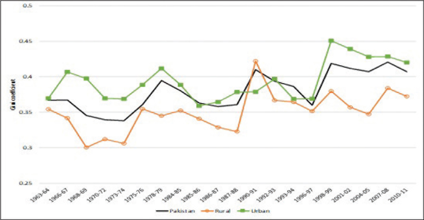
Pakistan has opted for the trade liberalization strategy in 1988 with the first structural adjustment program of International Monetary Fund, and trade liberalization witnesses even higher escalation in 1995 but income inequality seems to increase over the last four decades despite marginal economic growth and trade liberalization episodes as shown in Figure 1.
Moreover, there are only a few studies based on the welfare analysis of agriculture trade liberalization for Pakistan’s economy. For instance, Iqbal et al. (2017) linked social accounting matrix (SAM) of Pakistan for 2008 and MyGTAP model to simulate the results of agriculture trade liberalization along with Pakistan’s multilateral and bilateral agreements. They tested three scenarios of 50% and 100% reduction in import tariff and export tariff for all tradable in each region, respectively, and eliminating import tariff and export subsidies on agricultural sector. They suggested an overall improvement in welfare mainly due to a decrease in import prices and increased consumption. Moreover, all urban households gained in terms of income but results are mixed for a rural household. Large and medium-sized rural households remained beneficiaries in terms of land income while small rural farmers and other non-farm rural households were on the losing side. Similar conclusions were made by Khan et al. (2015) for Pakistan. Such findings, therefore, can have serious concerns regarding income inequality.
The results of each research remained mixed and further, it can be argued that these studies simulate liberalization scenario on the whole economy rather than liberating only agriculture sector. Therefore, positive gain for agriculture sector in the latter study might arise from impact of trade liberalization of non-agriculture sectors.
Due to a particular backdrop in previous literature, this research intended to quantify the impact of trade liberalization and trade protectionism predominantly on the Pakistan agriculture sector. For said purpose, computable general equilibrium (CGE)-based MyGTAP model is employed for understanding the impact of two contradictory policies on macroeconomic indicators (real gross domestic product [GDP], government income, terms of trade, etc.), trade, sectoral production, real income and income inequality. It is important because the effect of agricultural trade liberalization on welfare is highly contested in the development economics literature (Cassel & Patel, 2003; Rakotoarisoa, 2011). Moreover, agricultural trade liberalization may also cause some negative socioeconomic impacts. Left unaddressed, these can impose serious challenges to the sustainable development of less-developed rural economies like Pakistan.
The rest of the article includes Section II describing material and methods followed by simulated results in Section III. Further, concluding remarks are provided in Section IV.
Computable General Equilibrium (CGE) models are simulation tools used by economists and policymakers worldwide. CGE modeling is frequently employed for simulation-based analysis because it assists in the estimation of the impacts of different trade policy changes (Lakatos and Walmsley, 2012; Khan et al., 2018). The main advantage of this model is its potential to associate the cross sectoral linkages within various sectors of the economy. Even some economists, like Burfisher (2017), Dixon and Jorgenson (2012) and Cardenete et al. (2012), classify CGE models as the analytical approach that sees the economy as a comprehensive system with components that are related to one another (industry, households, investors, governments, importers and exporters).
GTAP Model
Like each family of CGE model, the standard GTAP model utilized an exhaustive list of mathematical equations to specify the functional form of the behaviour and characteristics of multiple economic agents following several theories regarding production technology, producer and consumer choices, the structure of private and public final demand, the zero profit and market clearance conditions and so on (Avinas & Norman, 2002). This study does not intend to discuss standard GTAP in detail (see Hertel, 1997 for complete structure of GTAP model), but necessary equations for the extension of standard GTAP model can be briefly articulated as follows.
MyGTAP Model
Minor and Walmsley (2013) made an extension to the standard GTAP model by removing a single regional household and replacing it with separate identities for government and private households. The extended model is known as MyGTAP model.
In MyGTAP model, taxes and foreign aid cashflows are now sources of income of the government. So, reginal government would receive foreign aid directly instead of a private household. Thus, net government income can be obtained by a difference between taxes, foreign aid cashflow and transfer from government to private households as shown in Equation (1).

Where, r ∈ REG, h ∈ HHLD.
GOVINC = Income earned by the government.
AIDI = Value of foreign aid inflows.
AIDO = Value of foreign aid outflows.
TTAX = Tax receipts.
TRNG = Transfers from the government to private households.
REG = Region.
HHLD = Private household.
Government utilizes the income (gincome) to meet government expenditures (yg), government savings (psave + qgsave or govdef). Where govdef is a notation for government deficit that is the difference between government income and consumption. In the core model, either government expenditure or government deficit is kept constant for simplicity. It is given as:


Where:
yg = Government expenditure. gincome = Government income in percentage change. qgsave = Real government saving/deficit. dpgav = Average distribution parameter shift for government. dpgsave = Government saving distribution parameter.
As shown in Equation (5), an income of a private household is given as income from factor endowment less depreciation. Further, net remittances along with transfers between households and government are also included in households’ income as:

Where, r ∈ REG, h ∈ HHLD, i∈ ENDW_COMM.
HHLDINC = Income of private household in level.
EVOAH = Earning from employing ‘i’ ENDW_COMM.
ENDW_COMM = Endowment commodities.
REMIH = Foreign labour remittances inflows.
REMOH = Foreign labour remittances outflows.
FYIH = Foreign capital income inflows.
FYOH = Foreign capital income outflows.
Following Cobb–Douglas functions, households spend their income to meet the demand for consumption and savings. Hence, accumulation of total savings by households (SAV_HHLD) and government (SAV_GOV) can be expressed in terms of regional savings as:

Where, r ∈ REG, h ∈ HHLD.
SAVE = Value of total regional savings.
qsave = Real savings.
qgsave = Real saving by government.
qhsave = Real saving by private household.
Multiple Households and Endowments
Various changes have to be considered to include multiple regional households into the standard GTAP model. First, identify the supply and possession of factor endowments by household and also adjust for the possibility of some factors being unemployed. Second, the inclusion of several additional types of endowments and third is to consider a transfer from household to government. The last point to consider is the possible difference between income and taxes on the commodity.
Let households have some level of factor endowments and supply it to the firm to earn income. The aggregate supply of endowments is an aggregation of endowment supplied by each household. Let us further assume that ownership of capital by household is known and hence household net income would be a difference between income and depreciation as shown in Equation (7).

Where:
qo = Total supply of endowments. SHREVOMH = Share of household in value of the endowment. qoh = Supply of endowment owned by households.
In MyGTAP model, it is possible to consider unemployment in macroeconomic closures and hence in Equations (8) and (9), emplh(i,h,r) and empl(i,r) denote the employment of labour by a single household or each household equally as:


Where:
qoh_s = Supply of endowment from household including unemployment. semplh = Employment of endowment from households. emplh = Shift parameter of employment of endowment from households. empl = Shift parameter of employment of endowment from households (equal across all households).
Once the supply of each endowment (qo(i,r)) is determined, we can label a particular endowment as a mobile or sluggish endowment. Further, MyGTAP model fulfils the necessity of separating endowments concerning their demand. As homogenous endowments from different locations are less likely to be easily substitutable, we can split such endowments to separate the demands for homogenous endowments that belong to different locations. After the said extension and splitting endowments, no changes were required to the underlying standard GTAP model.
Further, MyGTAP model allows us to incorporate multiple households for one country and leave regional households as such for other regions that are not of much importance to our analysis. Thus, provides essential flexibility for reducing data requirements.
Model Closure and Decomposition of Regional Welfare
The particular study employed the method of equivalent variation (EV) for quantifying the welfare decomposition as documented in Huff and Hertel (1996). Instead of utilizing regional household’s expenditure function, the procedure consists of changes in terms of trade and various efficiency sources. Equation (10) can express the EV measure as:

Finally, the solution of the model requires the exogenous variable to be equal to endogenous variables. Closure of the model consists of markets in equilibrium where a firm has zero real profit and consumers are on their budget constraints. Furthermore, employment is assumed to be full.
Particular policy scenario changes the parameters of the model, thus results in a shift from original equilibrium to a new equilibrium level. The change in equilibrium level is measured and termed as the impact of a particular policy.
Data Requirements
CGE-based models usually require exhaustive data requirements and most of the CGE models used SAMs to quantify the impact of particular policies. However, GTAP made an excellent effort in obtaining and collecting all of the required data in the form of input–output tables of 140 regions. GTAP Data Base also provides data of bilateral trade for 57 commodities, services and intermediate inputs among sectors. Furthermore, data on taxes and subsidies imposed by the governments are also given. Other than that, Data Base presents data on consumption, production and international trade (including transportation and protection data), energy data and carbon dioxide emissions for three benchmark years (2004, 2007 and 2011) (Aguiar et al., 2016). Tariff information has been converted into ad-valorem and for subsidy rates, domestic support payments have been used. Moreover, the different economic flows are taken in millions of current US$.
The particular study employed MyGTAP model that requires additional data to split a regional household into multiple households. 1 Therefore, we used SAM (2011) of Pakistan (constructed by IFPRI, 2016 2 ) and Household Income and Expenditure Survey (HIES) 2011 to extract data on different types of households and then integrate it into the GTAP Data Base version 9.2 with the reference year 2011. Further, Pakistan’s SAM (2011) is also used for splitting factors as shown in Table 1. Household types and their respective HH codes have been presented in Table 2. Method and tools of integrating SAM into GTAP Data Base are documented in Minor and Walmsley (2013).
Real Factors of Production and Their Codes
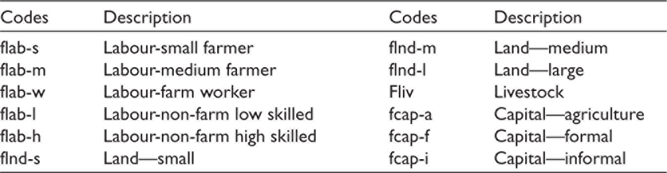
Household Types and Their HH Codes.

bSmall farms are less than 12.5 acres.
cMedium-large rural farms are greater than 12.5 acres.
dRural farmers operating land do not own land, but they operate farms for owners and hence earn returns on that land.
eRural farm workers work on farms owned and operated by others.
fRural non-farm workers work in rural areas but in non-farm occupations.
Measures of Income Inequality
This study further extended MyGTAP model to capture the changes in income inequality. Inequality can be defined as income gap among different households of a region (Litchfield, 1999). Out of several inequality measures, this study incorporated the following measures:
Gini Coefficient
GINI coefficient (Gini) is most widely used and easy to compute measure of inequality. It is based upon the comparison of the distribution of a variable (i.e., income, expenditure, etc.) with hypothetical uniform distribution (45-degree line) representing perfect equality. Gini ranges from 0 (perfect equality) to 1 (maximum inequality) and can be expressed as:

Where, r ∈ REG, h ∈ HHLD.
H = Total number of households in region ‘r’.
HHLDINC = Income of household ‘h’ in region ‘r’.
The Lorenz curve for selected 16 households based upon SAM (2011) provided by IFPRI (2016) is shown in Figure 2.

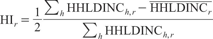
Hoover Index
Hoover index (HI), also known as the Robin Hood index, measures the vertical gap between Lorenz curve and 45-degree line of uniform distribution. HI also ranges from 0 (no redistribution required) to 1 (maximum redistribution required) and can be interpreted as a proportion of income need to be redistributed from household having income above the mean to those below the mean income of total households. HI can be articulated as:
Simulation Designs
Experiments are designed to evaluate agriculture trade liberalization/protectionist policy as a tool of boasting up the income of households associated with agriculture. At a macro level, the performance of policies will be evaluated by the change in indicators such as government income, GDP, terms of trade, volume of import and export and income inequality. Last but not least, method of EV will be used to determine the change in overall welfare linked with a particular trade policy. The scenarios under examination are as follows:
For agricultural trade liberalization, we reduce ad-valorem tariff by 10%. Similarly, we increase ad-valorem tariff rate by 10% for simulating the impact of trade protection. The main objectives of these experiments are to compare the effectiveness of both contradictory policies in reducing income inequality in the case of Pakistan’s economy.
The aim of this particular study is to quantify the impact of agricultural trade liberalization and protection on sectoral production, within household income redistribution and income inequality. Ad-valorem tariff on the imports of primary agriculture sector of Pakistan has been increased and decreased by 10% in order to carry out the simulations.
Impact on Macroeconomic Indicators
Table 3 demonstrates an increase in government income as a result of both simulations. The government earns extra tax income by 0.05% due to a 10% increase in import tax. But surprisingly, reducing import tariff by 10% also results in a 0.02% higher government income possibility because of the surge in import volume by 0.13%. Real GDP increased by $5.078 million due to trade liberalization and declined by $3.05 million in case of trade protection. Rise of export volume by $8.65 million causes real GDP to rise by only 0.002% because imports also rise by 0.13% in volume due to liberalization. Though an increase in import volume by $73.02 million is higher than the increase in export volume, even then terms of trade still manage to improve due to rise in export prices by 0.11% as compared to 0.001% decline in import prices.
Change in Macroeconomic Indicators
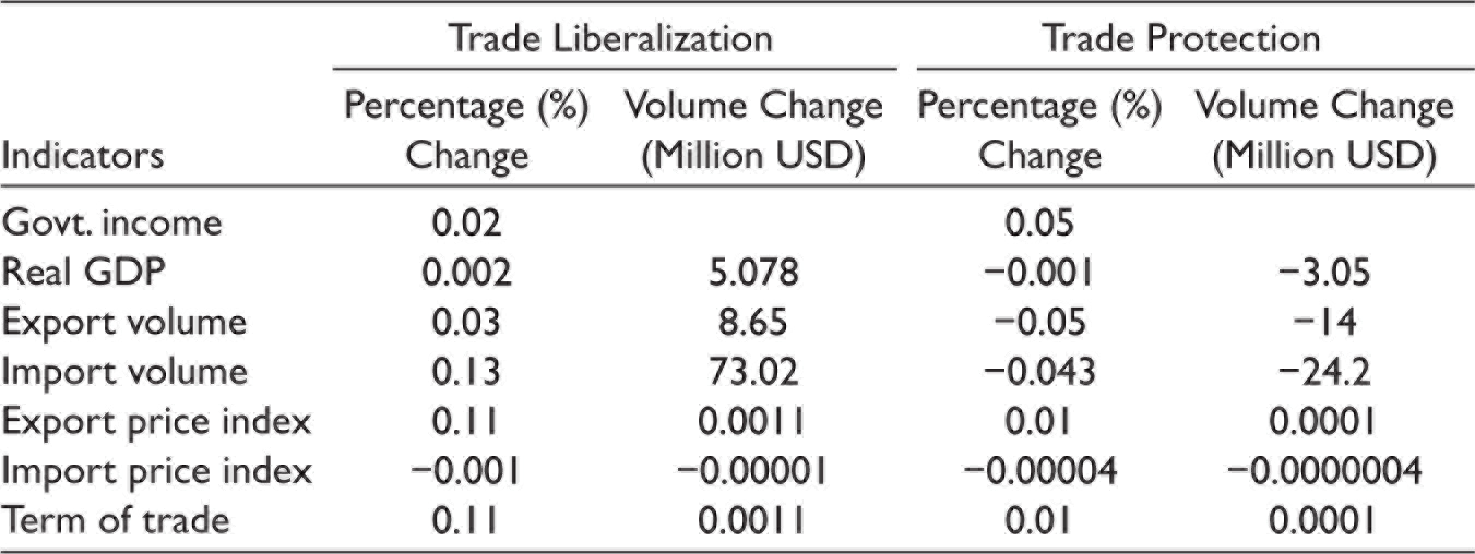
Change in Macroeconomic Indicators
Protection costs Pakistan $3.05 million worth of real GDP mainly due to a decline in export volume by $14 million. Decline of import volume by $24.2 million seems to be not enough to overcome the loss but due to an increase in export prices by 0.01% as compared to 0.00004%, decline in import prices term of trade improved slightly by merely 0.01%. Therefore, terms of trade in GTAP framework depend upon international export and import prices rather than volume of exports and imports.
Sectoral Impacts
Impact of primary agricultural liberalization and protection on sectoral production in Pakistan is provided in Table 4. Each major sector of Pakistan’s economy shows positive impact of trade liberalization except for agriculture value-added sectors such as textile and wearing apparel (TexWapp). Despite the processed food sector contributing positively, yet the loss of textile production out-weight the respective gain of production of processed food. Among primary agriculture, vegetable and fruit sector is a leading contributor in gain from higher level of trade.
Change in Sectoral Output
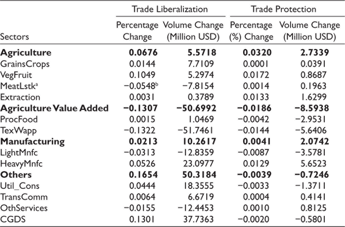
bDecline in output implies higher reliance on imports in order to satisfy total consumer demand.
Meat and livestock (MeatLstk) sector incurs output loss by 0.06% but overall, primary agriculture sector gains in terms of domestic output by 0.07%—$5.6 million worth of output. Primary agriculture sector remains gainer in the case of trade protection as well but the benefit is significantly lesser as compared to that of liberalization. Despite each sector of primary agriculture contributed a little in higher production but overall agriculture sector managed to increase the output by $2.73 million.
It is worth stating that the primary or secondary agricultural sectors like meat and livestock and textile and wearing apparel exhibit decline in output in case of 10% rise in liberalization. Table A3 shows that on average Pakistan has adopted relatively higher level of protection to these sectors against the world as compared to the protection provided by the world against Pakistan’s export of particular sectors. On the other hand, import tariffs on all of the other agricultural imports of Pakistan are lower than tariffs imposed on Pakistan’s exports to the foreign countries. Therefore, we can expect a decline in sectoral output of Pakistan, if the import tariff imposed by Pakistan is higher than the tariff imposed on particular sector of Pakistan by foreign countries. Further, it can also be incurred that MeatLstk and TexWapp sectors are less competitive in domestic market as compared to other agricultural sectors and hence, needed higher level of protection in order to enhance output on the expense of consumer surplus.
The increase in production in case of liberalization and protection can be explained by increase in demand for Pakistan’s product in domestic or foreign market; however, reason for demand increase might differ in both cases. Liberalization increases export volume and lowers the prices of agricultural products along with other sectors of Pakistan, which results in higher consumer demand in domestic and foreign markets as well. On the other hand, protecting agricultural sector causes import prices to rise and compel domestic consumers to substitute from imported products to domestic products.
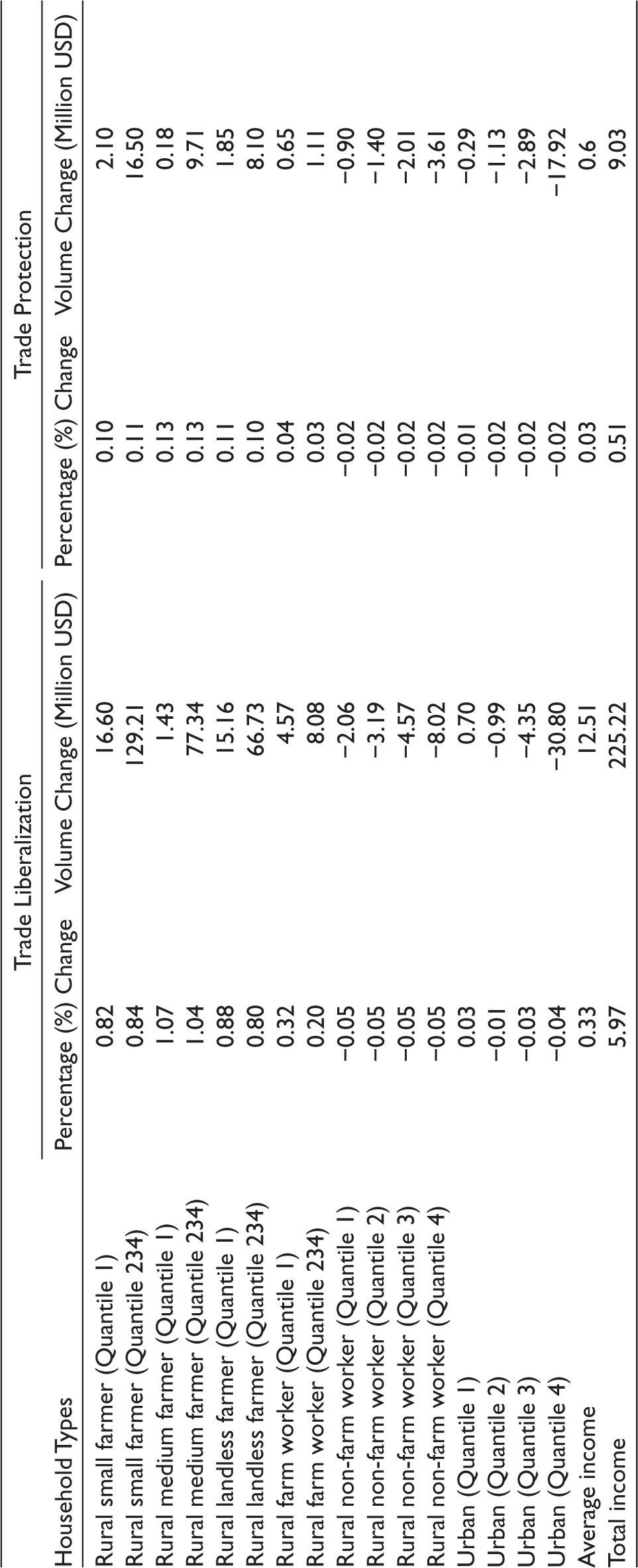
Increase in agricultural production benefits richer farmers 3 belonging to rural segment of Pakistan. The grain crop being the largest agriculture sector played vital role in income redistribution caused by any trade policy. Farmers 4 with medium-sized farms are the leading beneficiaries of trade gains followed by small farmers and landless farmers. The income of farm workers also increased due to the increase in the availability of jobs but non-farm workers lose their income by 0.05% in each province of Pakistan.
Surprisingly, urban households of Punjab also gain in terms of real income and urban households from the provinces other than Punjab lose part of their income that might increase income inequality among urban population across the provinces. Similar patterns can be observed in case of agricultural protection but the magnitude of the gains is much smaller and significantly larger in case of losses. However, there is an exception that in case of protection, urban household from Punjab might also join urban households from other provinces and non-farm workers as losing side.
It is worth mentioning here that meat and livestock is an important source of income for poor rural households along with wages from their services in farms. Hence, decline in meat and livestock production can significantly hurt those poor rural households, but in case of liberalization the higher wage resulted from increase in production of grain and vegetable and fruit sectors out-weight the possible loss that might have caused by lowered meat and livestock production. Moreover, despite increase in output of meat and livestock in case of protection, the increase in income of poor rural households remained low as compared to that in case of liberalization as shown in Table 5. This might imply that meat and livestock do not determine the income of rural farm workers to the great extent.
Change in Real Income by Household Types
Impact on Income Inequality and Welfare
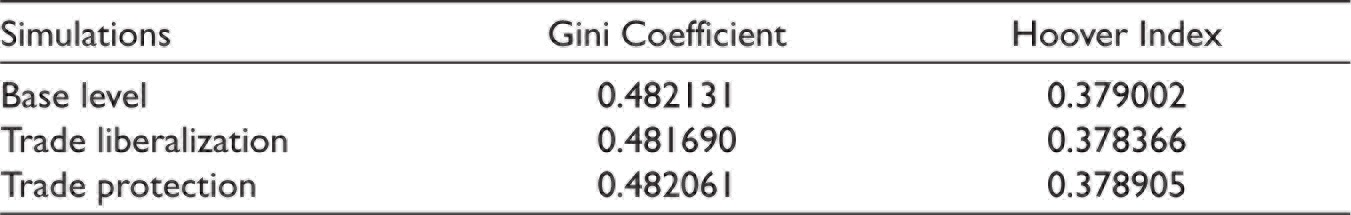
Tables 6 and 7 present the impact of both simulations on income inequality and welfare, 5 respectively. In both simulations, inequality reduces but with differing magnitudes. A total of 10% higher level of trade liberalization reduces inequality more because raise in domestic output is comparatively larger than in case of output raise in case of protection. But production increases in both cases, therefore income inequality reduces in both cases. Moreover, both measures of income inequality have revealed similar results in each simulation.
Change in Income Inequality
Change in Public Welfare
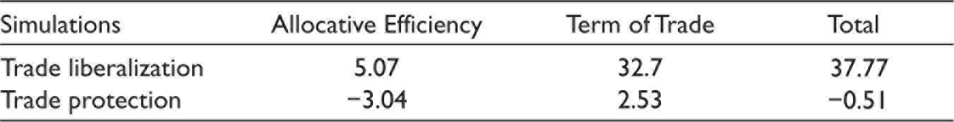
Further, terms of trade improved by $32.7 million and $2.53 million in case of liberalization and protection, respectively. However, protection results in allocative inefficiency that might cost $3.04 million and even offsets the gain from improved terms of trade and results in loss of public welfare by $0.51 million. On the other hand, liberalization improves the allocation of the factors of production and adds $5.07 million to the public welfare and hence, benefits the public by increasing their welfare by a total of $37.77 million.
From the above experiments, it can be noticed that neither change in public welfare nor change in real GDP is a good indicator for assessing the impact of trade policies on income redistribution or income inequality.
In most developing economies, the agricultural sector is of key importance to the economy as a whole. It represents the main source of income for the majority of the population. Besides, through substantial contribution of this sector to GDP and export earnings, it determines the course and the success of the overall process of economic development, especially in the less-developed countries like Pakistan.
Almost 70% of Pakistan’s population is directly or indirectly linked with agriculture and 48% of labour force is estimated to be engaged directly with agriculture. Agriculture sector is not only the major source of food for mass population but also contributes 25% in whole GDP of Pakistan which is highest among other sectors.
These facts have been well-known to Pakistan researchers for years. More recently, they have been substantiated by the findings of econometric analyses of the interrelationship between agricultural production and the growth of the economy as a whole but yet there are not many comprehensive empirical studies that focus on implications of agriculture trade policies on agriculture sector of Pakistan, economy as a whole and especially on income distribution among poor rural segment. There is qualitative research in this area that only shows one side of the picture or focuses mostly on industrial sector with secondary focus on agriculture sector.
This particular study focuses primarily on agriculture sector and quantifies the welfare impact of liberating and protectionist trade policies on agriculture at sectoral level. We utilized extension of the standard GTAP model and GTAP Data Base version 9.2 with base year 2011 and also employ Pakistan’s SAM (2011) and HIES (2011) to split households into 16 categories to grasp the distributional impact. Among 16 categories, there are 12 categories of rural households. This enables us to examine the distribution of income across the rural household. Finally, Gini coefficient along with HI is utilized to capture the impact of particular policy on income inequality in the case of Pakistan.
The simulated results suggested that Pakistan macroeconomic indicators such as real GDP, export and import volume, terms of trade performed better in case of agricultural trade liberalization. At sectoral level, agricultural production increased in both simulations but the rise in output turns out to be smaller in case of 10% decline in agricultural liberalization. However, caution is required as sectoral output can decline as a result of higher liberalization if a sector is relatively more protected against the world as compared to the protection provided by the world against particular sector of Pakistan.
In both cases, richer rural households gained extra income from higher output of grains crops, vegetables and fruits. However, the particular gain is once again higher for trade liberalization. Further, the poor farm workers also enjoy higher income that resulted from higher wages due to increase in the availability of jobs in grain crops and vegetables and fruits sectors.
However, poor rural farm workers also rely on livestock as a source of income and trade liberalization reduced the meat and livestock output but the higher wages offset the negative impact of decline in meat and livestock performance. Agriculture sector under protection, however, results in increase in the production of meat and livestock but even then overall increase in output remained lesser as compared to that in case of liberalization. Households other than farmers and farm workers turned out to be losers in both simulations. But the losses to the losers are greater in case of 10% decline in trade liberalization.
Impact of agricultural liberalization or protection on income inequality turned out to be unclear as in both scenarios, income equality declined. Magnitude of decline might be greater when Pakistan opted for 10% increase in trade liberalization but statistically not very different. Therefore, this study cannot suggest agricultural trade liberalization as an essential remedy for the cure of income inequality in case of Pakistan. Additionally, income inequality seemed to be directly related to agricultural production rather than trade liberalization or trade protection but trade liberalization might help agriculture sector comparatively more in order to boost its output through increase in demand among domestic and foreign consumers.
Unlike results of income inequality, estimates of equivalence variance clearly suggested agricultural trade liberalization as a dominating policy for raising public welfare as a whole. Apart from standard results, particular study also pointed out that neither public welfare nor real GDP can be a good indicator of assessing potential impact of trade policies on income inequality.
Footnotes
Declaration of Conflicting Interests
The authors declared no potential conflicts of interest with respect to the research, authorship and/or publication of this article.
Funding
The authors received no financial support for the research, authorship and/or publication of this article.
Appendix
Average Import Tariffs by Sectors

| Sectors | Import Tariff Imposed on Pakistan | Import Tariff Imposed by Pakistan |
| GrainsCrops | 24.99 | 2.55 |
| VegFruit | 8.81 | 3.40 |
| MeatLstk | 3.95 | 4.41 |
| Extraction | 8.49 | 6.05 |
| ProcFood | 8.23 | 14.14 |
| TexWapp | 10.20 | 10.26 |
| LightMnfc | 7.13 | 11.29 |
| HeavyMnfc | 12.86 | 9.24 |
| Util_Cons | 0.00 | 0.00 |
| TransComm | 0.00 | 0.00 |
| Services | 0.00 | 0.00 |
| Total | 68.66 | 61.35 |