Exploring the Relevance of Crude Oil Prices and Installed Generation Capacity in Prognosticating the NIFTY Energy Index

Abstract

The article brings a new approach with a proficient rendition of the existing literature emphasizing the stock and oil prices (OP) nexus, and it uniquely incorporates the demand-side impact of the domestic electricity installed capacity (IC) on India’s benchmark NIFTY Energy Index (NEI). The study undertakes a multivariate time series analysis consisting of a dual-cointegration exercise with the Johansen test and the Bounds test followed by a comprehensive residual analysis. From the multivariate analysis, the study found that the underlying variables are having a significant long-run association among them, while with Granger causality test, it detects a bidirectional causality in the case of IC and energy index pair, and no significant causality in the case of crude OP and energy stock returns pair. After this, the study proceeds with a univariate analysis of a long time series and establishes that the NEI can be foreseen with a suitable ARMA model and residual heteroscedasticity EGARCH analysis even in the presence of exogenous shocks.

Keywords

NIFTY Energy Index crude oil price electricity installed capacity dual-cointegration analysis residual analysis

I. Introduction

Petroleum oil price (OP) in the modern context of development is of huge importance as an aspect that possibly can be the most powerful source of all the economic uncertainties (Rotemberg & Woodford, 1996). For obvious reasons, there are a plethora of research works dedicated to studying the impacts and implications of OP movements on various spheres of the economy and from different dimensions of analysis (Murshed et al., 2021; Ul Husnain et al., 2021). As far as the financial economy is concerned, an upsurge in the OP induces higher production costs, which generally increases inflation and dampens consumer confidence in the market and also leads to volatility in the stock prices (Noor & Dutta, 2017). From the older studies, Jones and Kaul (1996) showed that innovations in OP in the post-war period of 1947–1991 adversely impacted the stock prices in the United Kingdom, Japan, the United States and Canada. The connectedness of crude OP with the capital market is also an emergent issue of analysis because, for the financial investors, the risk-spillover effects stemming from the OP fluctuations influence the tendency to hedge their portfolios, which may bring momentous consequences for the market as a whole (Batten et al., 2017; Cevic et al., 2020).

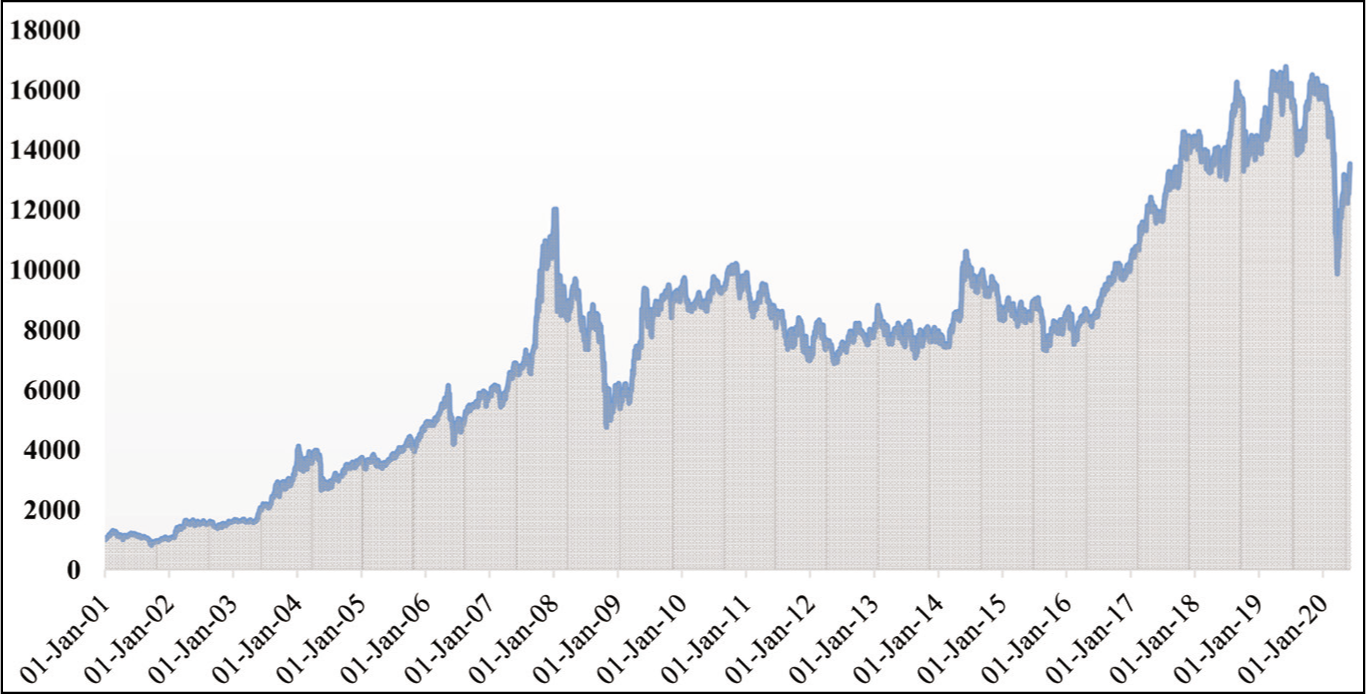
The NIFTY, as the benchmark index of India’s National Stock Exchange (NSE), launched in April 1996, comprises a well-diversified 50 companies across 14 sectors and represents 66.8% of the free-float market capitalization¹ of the stocks listed on NSE as on 29 March 2019; hence, it reflects the financial health of the listed universe of Indian companies (NSE website). As a sectoral index under NIFTY50, the NIFTY Energy index (NEI) was launched on 1 July 2005, with a base value of 1,000 counted from 1 January 2001 to represent the behaviour and performance of the Petroleum, Gas and Power sector. With an approximate ₹17.68 trillion market capitalization and a beta of 0.96 (correlation of 0.85) with the benchmark NIFTY50 index since its inception, the NEI ensured a price return of 14.15% so far, signifying its importance in the Indian capital market. Figure 1 shows the movement of the NEI and portrays its promising growth trajectory to ruminate the performance of the Indian energy sector in the last two decades, especially after 2015 with a steep rise in market cap.

Figure 1.

Source: NSE Factsheet.

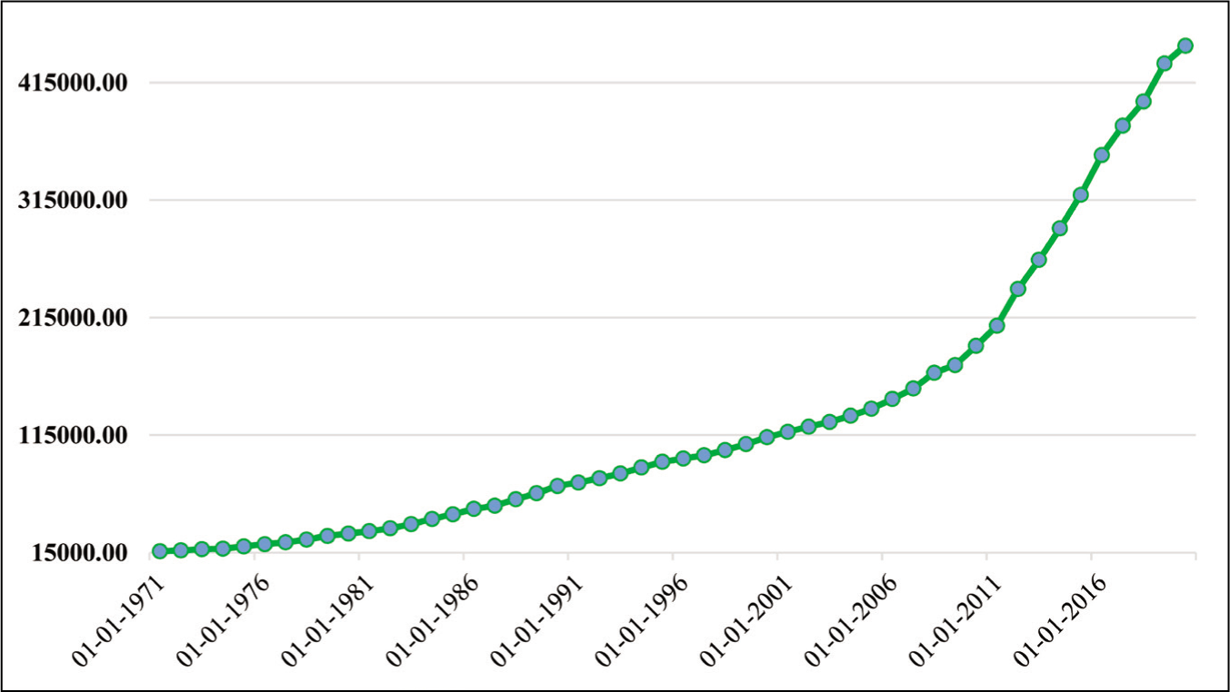
The present study overcomes a major limitation of almost all the previous researches, which are found to be ignoring the demand-side determinants of the stock returns. While dealing with the energy stocks, the installation of new generation capacity could be the yardstick to capture this signal for the industries to respond with more demand for funds from the capital market. Figure 2 shows the pattern of increased electricity installed capacity (IC) in India for the last five decades. The convex shape of the curve in this figure indicates the steepness of this increase and vindicates its importance as a determinant in the sphere of India’s energy industries. Hence, this study includes the electricity IV in an in-depth multivariate analysis of the benchmark index of India for the possibility of better forecasting and even predicting the market sentiments, which to the best of information, has never been done so far.

Figure 2.

Source: CEIC Insights.

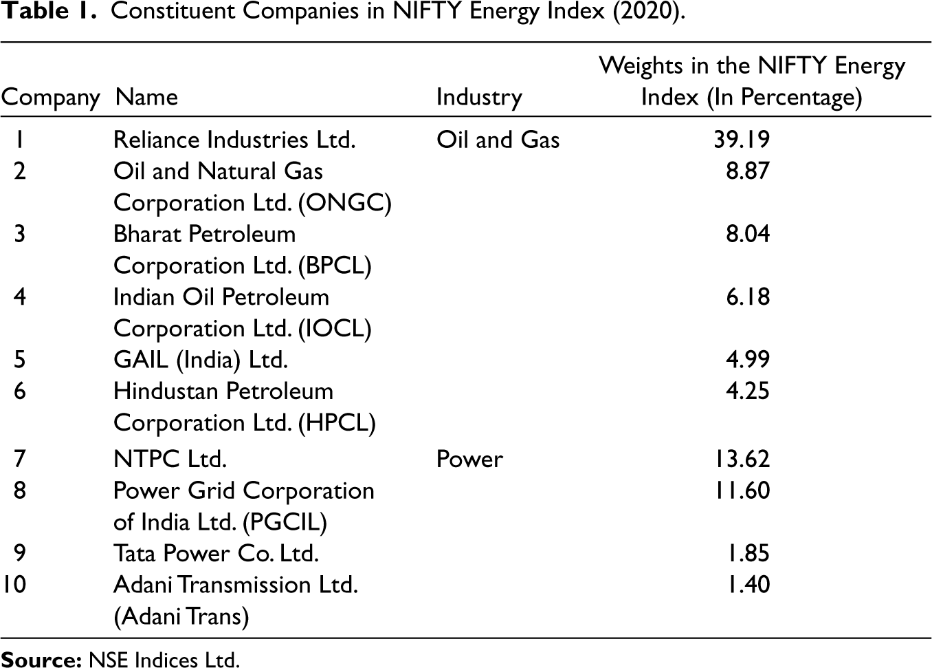
The coverage of the NEI is shown in Table 1. According to this table, the energy index is constituted of 10 big companies belonging majorly to two industries. The industry of Oil and Gas contributes around 71.88% as the weight in the NEI. On the other hand, four companies from the Power industry also contributes to around 28.12%. This substantial contribution of more than one-fourth in the index value from the Power industries is another major reason to consider the installed generation capacity in this present analysis as a potential determinant to influence the NEI. Hence, the novelty of the study lies in its first-ever systematic attempt to establish multivariate short-run and long-run relationships concerning the energy stock prices in an Indian context.

Table 1.

Constituent Companies in NIFTY Energy Index (2020)

Company Name		Industry	Weights in the NIFTY Energy Index (In Percentage)
1	Reliance Industries Ltd.	Oil and Gas	39.19
2	Oil and Natural Gas Corporation Ltd. (ONGC)		8.87
3	Bharat Petroleum Corporation Ltd. (BPCL)		8.04
4	Indian Oil Petroleum Corporation Ltd. (IOCL)		6.18
5	GAIL (India) Ltd.		4.99
6	Hindustan Petroleum Corporation Ltd. (HPCL)		4.25
7	NTPC Ltd.	Power	13.62
8	Power Grid Corporation of India Ltd. (PGCIL)		11.60
9	Tata Power Co. Ltd.		1.85
10	Adani Transmission Ltd. (Adani Trans)		1.40

Source: NSE Indices Ltd.

The article is structured as follows. Section II briefly represents a review of previous researches. Section III discusses the methodological details. Section IV elaborates the data sources used in the empirical exercises. Section V explains the results and derives implications therein to elaborate on the contribution of this study. Finally, Section VI concludes the study.

II. Literature Review

The OP and stock returns nexus is extensively addressed in the literature to improve the predictability in the capital market (Arouri et al., 2011; Arouri & Rault, 2010; Bondia et al., 2016; Kang et al., 2014; Narayan & Gupta, 2015; Sadorsky, 2014; Salisu & Isah, 2017; Salisu et al., 2019; Swaray & Salisu, 2018). One popular research domain that originated from this nexus is exploring the sustainability aspects of energy generation and use (Banerjee, 2019, 2020, 2021a; Banerjee & Murshed, 2020). On the other hand, this nexus is particularly examined in terms of clean energy stocks (Bondia et al., 2016; Henriques & Sadorsky, 2008; Managi & Okimoto, 2013; Sadorsky, 2012; Wurzburg et al., 2013), and technology stocks (Maji, 2015; Omri et al., 2015) due to the possibility of energy substitutions and technology adoptions in response to the increased OP (Ahmad, 2017; Banerjee et al., 2021a; Kumar et al., 2012).

However, the research direction so far is found mostly motivated in the capital markets of the United States (Dutta, 2017a, 2017b; Ferrer et al., 2018; Ghosh et al., 2019; Killian & Park, 2009; Managi & Okimoto, 2013; Salisu & Okolo, 2015; Salisu et al., 2019; Vo, 2011) and the European countries (Arago-Manzana & Fernandez-Izquierdo, 2007; Asteriou & Bashmakova, 2013; Cunado & Perez de Gracia, 2014; da Silva et al., 2016; Oberndorfer, 2009; Wurzburg et al., 2013). A handful of research is also devoted to studying the impact of OP movements on the stock markets of Australia, China, the GCC countries, Japan, Jordan and Lebanon (Arouri & Fouquan, 2009; Bouri, 2015a, 2015b; Faff & Brailsford, 1999; Kawashima & Takeda, 2012; Wei et al., 2019). Batten et al. (2016) considered the relationship between energy and stock prices both individually and as an energy portfolio in the context of China and Japan, and they found that in the post-global financial crisis period, Asia’s important stock markets moved in tandem with OP. Using weekly data of 1990–2017, Cevic et al. (2019) could not find crude OP significantly impacting the stock market returns in the case of Turkey in terms of their entire sample; however, they substantiated that there are significant spillover effects from crude OP changes to stock market returns during the crisis phases of 1993 and 2008–2009. Sun et al. (2018) explored the impacts of three fossil energy (coal, oil and natural gas) prices on new energy companies’ stock prices of China and found that previous stock prices of new energy companies had the most significant impact on the base level, but that the fossil energy prices account for only a small part of stock price fluctuations of new energy companies.

The review of the existing literature, however, found the aspect of OP–stock prices nexus inadequately addressed in the Indian context (Upadhyay, 2019). Rigorous investigation on this aspect is felt to not only predict the capital market fluctuations but also address the clean energy transition issues from private investment viability and international negotiation on emission mitigation perspectives (Anbumozhi et al., 2018; Banerjee, 2021b, 2021c; Banerjee et al., 2021b). Using an integrated non-parametric framework, Ghosh et al. (2019) investigated the co-movement and dynamic correlation of the financial and energy markets in the context of NIFTY and BSE Energy Index, and they brought new insights for portfolio management to mitigate risks. In a different study, Ghosh et al. (2018) considered the daily data of crude oil and natural gas prices. The NEI and US Dollar–Rupee exchange rate, however, brought only a methodological contribution that can be used for effective forecasting of the causal influences.

This study begins to fill a gap in the existing body of the literature by introducing a comprehensive investigation about the predictability of India’s stock market index in response to the overtime change in crude OP and the demand-driven factor of installed electricity generation capacity. Moreover, this study authenticates its analytical framework concentrating on the sectoral index, which is constituted with the stocks of only the energy industries and shows how this drives to predict the sectoral market sentiments.

III. Methodology

To empirically investigate how the power generation capacity and the crude OP are contributing to the NEI and to derive implications therein regarding how these contributions are acting as the potential drivers to predict the future market sentiments in the energy sector, the framework of this study may be divided into a two-fold time-series econometric exercise.

Primarily, the study explores the long-run relationship and the interactions of the NEI with the domestic electricity IC and the OP by conducting a multivariate exercise.

Null hypothesis (H₀): There is no long-run relationship between NEI, IC and OP.

Alternative hypothesis (H₁): There is a significant relationship between NEI, IC and OP.

After the multivariate exercise, the study conducts a univariate exercise to inspect how this index can be forecasted to predict the future movements in the stock prices of the energy sector.

Null hypothesis (H₀): NEI cannot be forecasted.

Alternative hypothesis (H₁): NEI can be effectively forecasted.

However, before conducting the econometric analysis, the study rigorously investigates and confirms the stability of the NEI. This is because the composition of the NEI in terms of contributing companies may significantly change over time. With major shuffles in this composition, the results from the econometric exercise may significantly be affected. To this objective of stability analysis, as market capitalization has historically proven to be the key indicator in identifying the gross contribution of any stocks into a composite index, the study evaluated similar market-cap-based contributions of the 14 stocks that appeared in the index under consideration for the last one decade. The analysis has been performed by preparing colour-coding-based heat maps using spreadsheet software. Besides, the study proposes to construct an alternative energy index comprising of those companies consistently contributing to the original NEI since the last decade. The study explores the near-similar trajectory of both the indices—the prevailing one and the proposed one—and signifies their correlational movement to substantiate the robustness of the results from the hypothesis testing in the presence of periodic changes in the NEI.

To establish the multivariate model for identifying the relationship, the study starts with a stationarity analysis exclusively by unit root tests with the help of the Augmented Dickey-Fuller (ADF) criteria to check the stochastic process in the variables under study such that their unconditional joint probability distribution does not change over time. Once the stationarity is identified, the variables are tested to assess the probable cointegration. The cointegration analysis is specified as follows in equation (1) in the form of a standard Vector Auto Regression (VAR) model of order p. Here, all the variables are transformed into their first difference log form² to better deal with the extreme values and for better interpretation of the results in terms of the independent variables. However, a suitable lag length is identified before performing the cointegration tests.

R N E I_{t} = A_{1} R N E I_{t -}_{1} + A_{2} R N E I_{t -}_{2} + \dots + A_{p} R N E I_{t - p} + B . R I C_{t} + C . R O P_{t} + ε_{t}

(1)

Here, RNEI_t is k-vector, RIC_t and ROP_t are the d-vectors of deterministic variables, and ε_t are the vectors of innovations. Therefore, the VAR may be expressed as follows:

Δ R N E I_{t} = \prod^{​} R N E I_{t - 1} + \sum_{i = 1}^{p - 1} Γ_{i} Δ R N E I_{t - i} + B . R I C_{t} + C . R O P_{t} + ε_{t}

(2)

Where: and $\prod^{} = \sum_{i = 1}^{p} A_{i} - I a n d Γ_{i} = - \sum_{j = i + 1}^{p} A_{j}$ ,

The cointegration analysis is initially conducted by the Johansen cointegration test. The VAR procedure, under the Johansen test, allows the simultaneous evaluation of multiple relationships and imposes no prior restrictions on the cointegration space. This procedure provides likelihood ratio tests based on the trace statistics and the Maximum Eigenvalue to test for cointegration. The study further investigates the possibility of cointegration among the underlying variables with the help of the bounds tests to cross-check the analysis and reinforce the conclusion drawn from the Johansen cointegration test. The autoregressive distributed lag (ARDL)-based estimation is applied for the short-run forecasting. An augmented ARDL bounds test for cointegration involves an extra F-test on the lagged levels of the independent variable(s) in the ARDL equation, and this testing strategy was introduced originally using the bootstrap procedure (Sam et al., 2019). The general ARDL model is written as follows:

\emptyset (L) y_{t} = δ + θ (L) x_{​} + υ_{t}

(3)

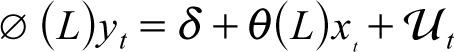
where $\emptyset (L)$ is an order-p polynomial that, for stability, has roots lying outside the unit circle and $θ (L)$ is an order-q polynomial. Expanding the lag polynomials, the following can be found.

y_{t} = δ + \emptyset_{1} y_{t - 1} + \dots + \emptyset_{p} y_{t - p} + θ_{0} x_{t} + θ_{1} x_{t - 1} + \dots + θ_{q} x_{t - q} + u_{t}

(4)

Therefore, the study performs the F-Bounds and the t-Bounds tests subsequently based on the ARDL consideration. The t-Bounds test, in particular, is a parameter significance test on the lagged value of the dependent variable. Since the distribution of this test is non-standard, the p-value provided in the regression output is not compatible with this distribution, although the t-statistic is valid and all the inferences are to be drawn using the t-Bounds test critical values. While the F-Bounds test will not have changed from the long-run form and the Bounds test view, the t-Bounds test here reflected the t-statistic associated with the regressors of the cointegration equation.

When the cointegration among the variables is established with both the tests with at least one cointegrating equation, the study proceeds with the Vector Error Correction model (VECM) to derive the long-run relationship. The VECM has cointegration relations built into its representation so that it restricts the long-run behaviour of the endogenous variables to converge to their cointegrating relationships while allowing for short-run adjustment dynamics.

To check the robustness of the VECM exercise, the study conducts a detailed residual analysis. VEC residual serial correlation LM test is performed to identify the possible correlation among residuals. A residual normality test is performed, and its significance is tested with Skewness, Kurtosis and Jarque-Bera values. Lastly, the residual heteroscedasticity test is undertaken to ascertain the innate nature of the residuals and the accuracy of forecasting the model.

In its second segment of the empirical exercise, this study conducts a univariate analysis with the NEI to investigate whether the stock prices can be forecasted to predict the future market sentiment in the energy sector. Here, the study tests the RNEI variable for its autocorrelation, which represents the degree of coherence or similarity between a given time series and its lagged versions over successive time intervals. The variable is tested with AR models of order 1, 2 and 3, and then the explanatory variable is tested with the Autoregressive Moving Average (ARMA) model of order (2, 2) as:

R N E I_{t} = c + ε_{t} + \sum_{i = 1}^{p} a_{i} R N E I_{t - i} + \sum_{i = 1}^{q} β_{i} ε_{t - i}

(5)

The error terms ϵ_t are generally assumed to be independent and identically distributed random variables sampled from a normal distribution with zero mean: ϵ_t ~ N (0, σ²), where σ² is the variance. This study tests the veracity of the ARMA (2,2) model and the significance of the lag variables using the Akaike information (AIC) criterion (Brockwell & Davis, 2009). After that, this study again performs the residual diagnosis to comprehend the nature and predictability of the error terms ϵ_t for more precise forecasting. This begins with understanding the possibility of heteroscedasticity amongst the error terms and then possible forecasting of the variance of the residual with a suitable statistical model. This study conducts the Exponential Generalized Autoregressive Conditional Heteroscedasticity (EGARCH) model to predict the RNEI. As proposed by Nelson (1991) that ϵ_t follows a generalized error distribution (GED)³, the specification for the conditional variance of EGARCH is as follows:

\log σ \begin{matrix} _{2} \\ t \end{matrix} = c + \sum_{j}^{a} β_{j} \log σ \begin{matrix} _{2} \\ t - j \end{matrix} + \sum_{j = 1}^{q} α_{j} | \frac{1_{t - 1}}{σ_{t - 1}} | + \sum_{k = 1}^{r} γ_{k \frac{ε_{t - k}}{α_{t - k}}}

(6)

The left-hand side is the log of the conditional variance, and it signifies that the leverage effect is exponential rather than quadratic and forecasts that the conditional variance is nonnegative. The presence of the leverage effects can be tested by the hypothesis that γ_i < 0. The impact is expected to be asymmetric if γ_i ≠ 0. The significance of the model is tested with not only the p-values of the model coefficients and ARMA variables but also with the results indicated by Akaike, Schwarz and Hannan-Quinn’s information criterion.

IV. The Data Sources

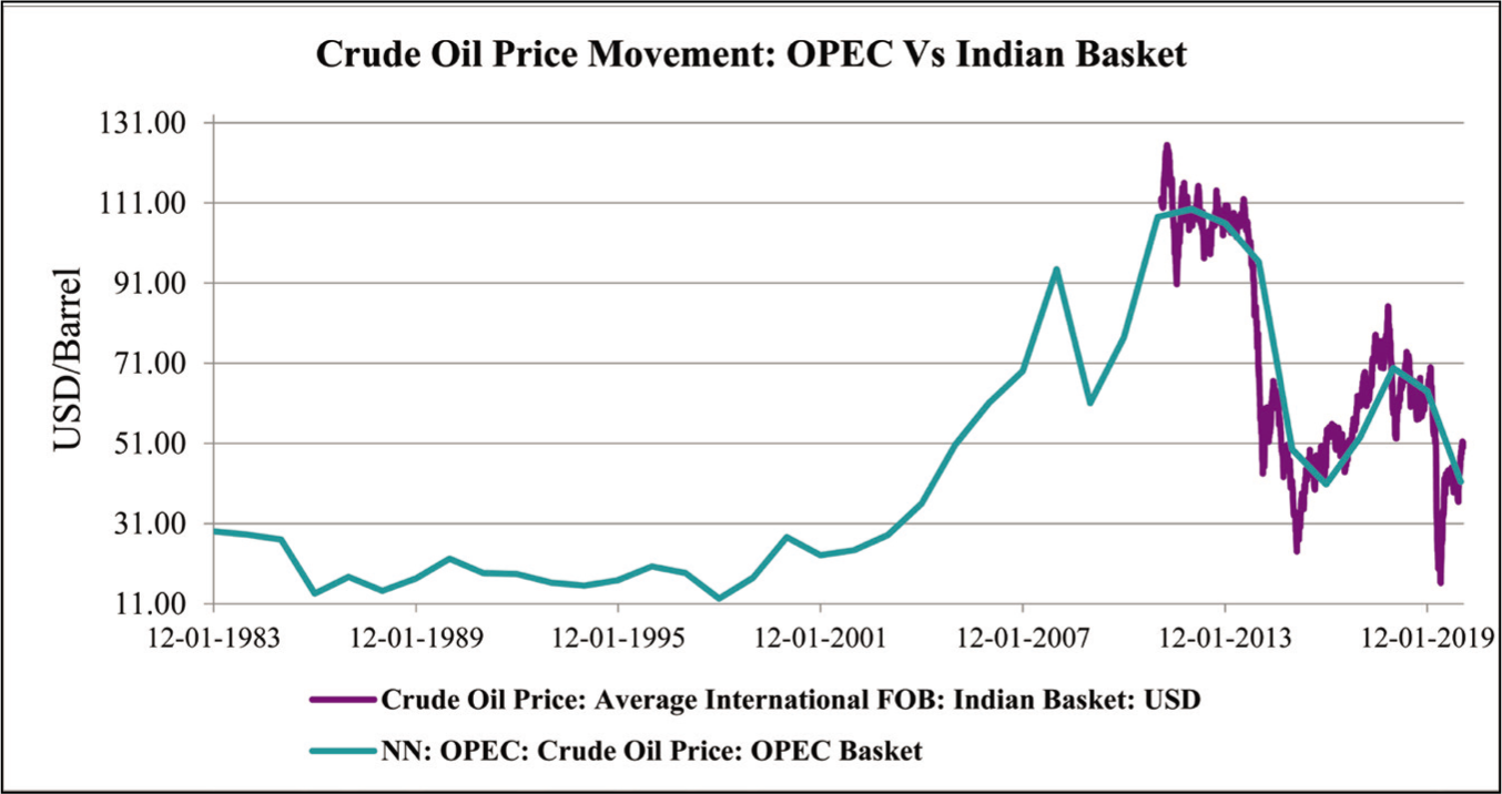
This study required multiple time series data points concerning the NEI, the electricity IC in India and the crude OP. For the multivariate analysis, this study used half-yearly based data points for all three variables from 2001 to 2019. The time series half-yearly data on the electricity IC in India since 2001 is gathered from the CEIC data repository. The crude OP data since 2001 is also obtained from the CEIC data portal where the OPEC basket data is considered for this analysis. The OPEC basket data is considered rather than the Indian basket because the former is found with more available data points. However, this study checked the correlation of the OPEC basket with the Indian basket of crude oil in terms of their price movements and found a strong correlation. Figure 3 emphasises their significant resemblance and shows consistency in the comparative movement of the OPEC and the Indian basket of crude OP, establishing the OPEC basket as a relevant independent data series for this analysis.

Figure 3.

Source: CEIC Insights.

For the univariate analysis, the daily data of the NEI is collected from the official data portal of the NSE of India. This analysis is performed with 4,746 data points from 1 January 2001 to 30 January 2020. For the construction of the alternative energy index, the study used financial data from the annual company financials of the individual companies that are consistently contributing to the existing NEI since 2014.

V. Results and Discussions

Stability of the NIFTY Energy Index

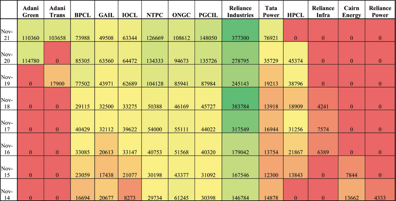
It has been ascertained that the composition of the NEI, constituted based on its free-float market capitalization considering that no individual stock contributes greater than 33% and the cumulative role of top three stocks shall not go beyond 62% at the time of rebalancing, has not been significantly altered over the years. An assessment of market capitalization of the NIFTY stocks under the Power and the Oil and Gas industry categories concludes that only 14 stocks appeared in the last ten years in composing the Index. The heat map as shown in Figure 4 depicts the comparative market cap volume of the stocks with an extraordinary consolidation over eight stocks. The green colour code signifies the higher market capitalization, which if eventually faded and successively turned into yellow and orange codes implies that the market capitalization is decreasing. On the other extreme, the red colour code implies the lowest market capitalization.

Figure 4.

Source: NSE Indices Ltd.

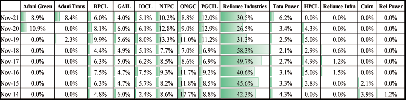
While digging deeper into the contribution of the gross market cap of those selected stocks to the overall energy index, this research zeroed in on the fact that eight stocks contributed to an average of 93% of the total energy index capitalization in the last decade. This aspect is portrayed in Figure 5, which reflects the percentage contribution of the total 14 stocks in the overall composition of the NEI since 2014. This finding not only strengthens the veracity of the index for this research but also conforms to its robustness for long-term sequential analysis.

Figure 5.

Source: NSE Indices Ltd.

Energy Index, Oil Price and Energy Generation Capacity

The study intends to find the long-run association of the NEI with the crude OP and India’s domestic electricity IC over time. The empirical exercise begins with testing the autocorrelation of the dependent variable ∆RNEI as indicated in equation (2) and the stationarity of all underlying variables RNEI, ROP and RIC. From the plots of autocorrelation and partial autocorrelation, RNEI is found to be autocorrelated at 1% significant level. The result of the ADF test for assessing the availability of unit root is represented in Table 2, showing rejection of the null hypothesis and implying that there is no unit root at first difference level for RNEI at 1% significant level. This confirms the stationarity of the variable RNEI and the possibility of forecasting it with a suitable empirical model. The ADF test of stationarity for the two explanatory variables RIC and ROP is also shown in Table 2, where the rejection of the null hypothesis declares these two variables as stationary with less than 1% level of significance.

Table 2.

Unit Root Test Results

Variables	Augmented Dickey Fuller Unit Root Test Exogenous: Constant
Variables	ADF Test Statistic	Prob.*	Lag-Length**
RNEI	−24.73678	0.0000	22
ROP	−4.981469	0.0013	0
RIC	−6.019588	0.0002	0

Source: The authors.

Notes: *MacKinnon (1996) one-sided p-values; **Based on SIC.

Table 3.

Johansen Cointegration Rank Test

		Unrestricted Cointegration Rank Test (Trace)		Unrestricted Cointegration Rank Test (Maximum Eigenvalue)
Hypothesized No. of CE(s)	Eigen Value	Trace Statistic	Prob.	Max Eigen-value Statistic	Prob.**
None*	0.920390	59.29879	0.0000	37.95923	0.0001
At most 1*	0.651952	21.93356	0.0047	15.83083	0.0280
At most 2*	0.334256	6.102761	0.0135	6.102761	0.0135

Source: The authors.

Notes: *Rejection of the hypothesis at 0.05 level; **MacKinnon-Haug-Michelis (1999) p-values.

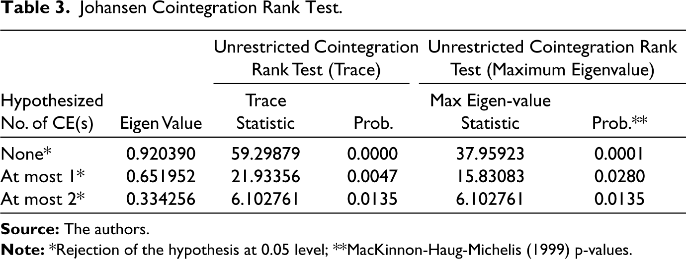
After the testing on the stationarity, suitable lag length is determined for further analysis of the variables. Hence an unrestricted VAR model is estimated considering RNEI as the dependent variable, whereas RIC and ROP are chosen as exogenous ones. This exercise found that the second order lag is the optimal length that is satisfying the Akaike, Schwarz and Hannan-Quinn selection criterion. Detection of the optimal lag order allows this study to further investigate the presence of a possible cointegration among the variables. This study applies the Johansen Cointegration test. Table 3 represents the outcome of the test where the cointegration is found established with three cointegrating equations at 5% level. This is emphasizing that the variables under study are cointegrated at a significant level and that there is a possibility of long-run forecasting of the dependent variable RNEI.

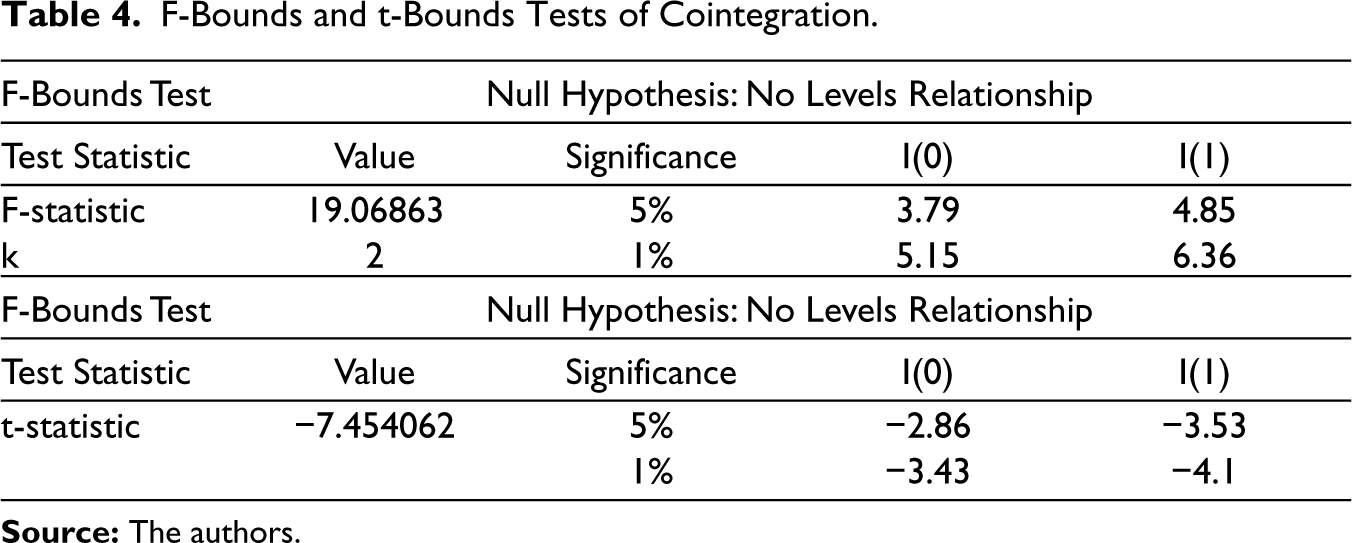
To reconfirm this possibility of cointegration and the opportunities for long-run forecasting, the F-Bounds and the t-Bounds tests are performed by considering an ARDL estimation of RNEI. Table 4 contains the details on the Bounds test results where the upper bound I(1) critical value of 6.36 at 1% significant level is much lower than the corresponding F-statistic that is 19.068, resulting in the rejection of the null hypothesis of no cointegration. The same can be revalidated with the absolute value of the t-statistic found to be 7.454 and is much higher than the corresponding I(1) critical value of 4.1 at 1% significant level. Hence, the study confirms the long-run relationship among the NEI, the Electricity IC and the OP with a very high significance level.

Table 4.

F-Bounds and t-Bounds Tests of Cointegration

F-Bounds Test	Null Hypothesis: No Levels Relationship
Test Statistic	Value	Significance	I(0)	I(1)
F-statistic	19.06863	5%	3.79	4.85
k	2	1%	5.15	6.36
F-Bounds Test	Null Hypothesis: No Levels Relationship
Test Statistic	Value	Significance	I(0)	I(1)
t-statistic	−7.454062	5%	−2.86	−3.53
		1%	−3.43	−4.1

Source: The authors.

The cointegrating relationship leads us to forecast the RNEI with VEC model. The Error Correction Term (ECT) is obtained from the Johansen cointegration test. Based on the result of this test, the ECT is ascertained as follows:

E C T_{t - 1} = R N E I_{t - 1} + 6.92098 R I C_{t - 1} + 0.1125 R O P_{t - 1} + ε_{t}

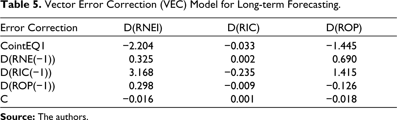
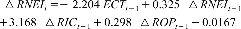
From this test, the coefficients of the independent variables with its respective error terms are found to be approximately 16 for RIC and 2 for ROP. Therefore, it can be concluded that the calculated ECT is significant. The same is revalidated through the significance of the ECT in the Bounds test result as well where the coefficients of both RIC and ROP are found to be significant at 5% level. The variables are modelled with the VEC model for subsequent forecasting of the dependent variable RNEI. The output of the VEC model is represented in Table 5 and can be written as the following. Here, the ECT_t–1, in this equation can be replaced with the representation obtained from its earlier equation.

Table 5.

Vector Error Correction (VEC) Model for Long-term Forecasting

Error Correction	D(RNEI)	D(RIC)	D(ROP)
CointEQ1	−2.204	−0.033	−1.445
D(RNE(−1))	0.325	0.002	0.690
D(RIC(−1))	3.168	−0.235	1.415
D(ROP(−1))	0.298	−0.009	−0.126
C	−0.016	0.001	−0.018

Source: The authors.

\begin{matrix} Δ R N E I_{t} = - 2.204 E C T_{t - 1} + 0.325 Δ R N E I_{t - 1} \\ + 3.168 Δ R I C_{t - 1} + 0.298 Δ R O P_{t - 1} - 0.0167 \end{matrix}

Once the multivariate analysis with the VECM is performed satisfactorily, the study further explores the sustenance of the model by diagnosing the model residual. The residual is first tested with the Serial Correlation LM test and subsequently with the VEC Residual Normality test as depicted in Table 6. In the top panel of Table 6, it is shown that the Serial Correlation LM test accepts the null hypothesis establishing no serial correlation among the residuals. On the other hand, the Residual Normality test is substantially found to be rejecting the null hypothesis of no normality with joint Jarque-Bera probability of 0.92 and Kurtosis probability of 0.86, as shown in Table 7’s middle panel. Hence, the residuals in the model possess considerable normality. After the serial correlation and normality testing, the residuals are subsequently tested for heteroscedasticity. Table 7’s bottom panel is showing that the residual heteroscedasticity diagnosis accepts the null hypothesis with a probability of 0.26 and signifying the residual as homoscedastic such that the basic model may be considered as sustainable. The cointegration analysis and the subsequent residual diagnosis only confirms the presence of long-run association and the short-run dynamics among the model variables, and establishes the robustness of the exercise; however, it does not indicate the direction of causality operating in this course.

Table 6.

Residual Diagnosis Tests

Residual Serial Correlation LM Test
Null Hypothesis: No serial correlation at lag 1 to h
Lag	LRE* stat	df	Prob.
1	10.38937	9	0.3199
2	3.956592	9	0.9142
VEC Residual Normality Test
Null Hypothesis: No residual normality
Component	Jarque-Bera	df	Prob.	(Kurtosis) Chi-square	df	Prob.
Joint	2.012537	6	0.9185	0.755939	3	0.8600
Residual Heteroscedasticity Test
Null Hypothesis: No residual heteroscedasticity (levels and squares)
Component	Chi-square	df	Prob.
Joint	53.66264	48	0.2663

Source: The authors.

Note: *Edgeworth expansion corrected Likelihood Ratio statistic.

Table 7.

Result of Pair-wise Granger Causality Test

Null Hypothesis	Observations	F-statistic	Prob.
RIC does not cause RNEI	17	8.77305	0.0103
RNEI does not cause RIC		3.20813	0.0949
ROP does not cause RNEI	17	0.09085	0.7675
RNEI does not cause ROP		0.06702	0.7995
ROP does not cause RIC	17	1.13462	0.3048
RIC does not cause ROP		3.09429	0.1004

Source: The authors.

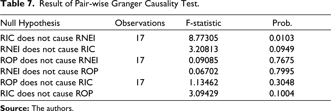
To inspect on the causality, this study conducts the pair-wise Granger causality test and the results are shown in Table 7. The results confirm that the RIC Granger causes the RNEI at 1% level of significance whereas the ROP doesn’t Granger cause the RNEI, signifying the RIC as a significant causal independent variable for RNEI. This finding is of notable importance due to its denial of causality between RNEI and ROP. A sizeable number of stocks of oil marketing companies in NEI, namely, IOC, HPCL and BPCL, are substantially benefitted with the dip in crude OP. These include, inter alia, improvement in marketing margin, increase in crude discounts from importing countries, reduction in gross input cost and lower working capital. On the other hand, a crude oil-producing entity like ONGC is negatively impacted with the fall in OP due to its high production cost and poor global competitiveness. Stock like RIL, catering to two-fifths of the index with petrochemicals contributing to 45% of its operating income and refining another 27.5% in FY 2019, are not benefitted with lower crude OP due to revenue erosion and significant swap/forward position in crude import. Table 7 reflects that RNEI also Granger causes RIC at a 10% level of significance, implying the possibility of a bi-directional causality between the two variables. This aspect is also important as far as its implications are concerned, since a stronger index, with one-fourth electricity production and transmission entities, may sustainably influence the electricity IC of India.

Predictability of the Energy Index

After arriving at the conclusion about the cointegration and causality among the model variables, this study uniquely investigates how far the NEI is predictable from its past values, provided there are exogenous shocks from outside the capital market. To this objective, the RNEI variable is first plotted to identify its distribution pattern and assess the possibility of regression modelling. The descriptive statistics for RNEI showing a near-normal distribution with short tail, slight negative skewness and considerably high Jarque-Bera with 4,745 observations, which permits this study for expected variable forecasting and residual modelling. Now the presence of autocorrelation in RNEI opens up the opportunity to test RNEI with first and second order autoregression AR(1) and AR(2) models. Both the models turned out to be insignificant in this case, resulting in the possibility of testing the variable with its residual terms. The ARMA model was checked to predict the RNEI with its past values and autoregressive error terms of first and second order lag. This study finds ARMA(2,2) model as the most appropriate in this case for RNEI. Table 8 represents the result of ARMA(2,2) modelling where all the coefficients are considerably found significant at 1% level, emphasizing the acceptability of the model. From these results, the generic ARMA (2,2) model can be represented for RNEI as follows:

Table 8.

Testing ARMA (2,2) Model for RNEI Variable

Variable	Coefficient	Std. Error	t-statistic	Prob.
C	0.000574	0.000245	2.340550	0.0193
AR(1)	−0.577571	0.094343	−6.122053	0.0000
AR(2)	−0.623811	0.058861	−10.59800	0.0000
MA(1)	0.656743	0.094063	6.981917	0.0000
MA(2)	0.642484	0.061153	10.50624	0.0000
SIGMASQ	0.000253	2.49E-06	101.5745	0.0000

Source: The authors.

\begin{matrix} R N E I_{t} = 0.000574 + ε_{t} - 0.577 R N E I_{t - 1} \\ - 0.624 R N E I_{t - 2} + 0.657 ε_{t - 1} + 0.642 ε_{t - 2} \end{matrix}

Once the ARMA(2,2) model is significantly established, the study checks the possibility of residual forecasting. Residuals are useful in analysing whether a model has adequately captured the information and trend in the data. Residuals contain information about the phenomenon modelled by function and about the goodness of fit (Vogel, 2010). A good forecasting method will yield uncorrelated residuals with zero means. The residual variations, the fitted plot and its comparison with the actual movement of RNEI variable reiterates the acceptance of the model and the necessity for residual analysis. The residual diagnosis starts with the assessment of the possible presence of heteroscedasticity through Autoregressive Conditional Heteroscedasticity (ARCH) test. The result of the heteroscedasticity test significantly rejects the null hypothesis of no heteroscedasticity at 1% level, resulting in the possible presence of heteroscedasticity in the residuals of RNEI forecasting model.

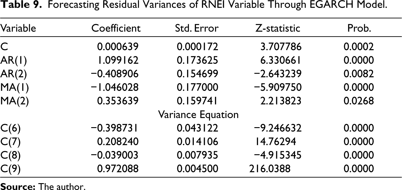
As the residual component can be demarcated to one stochastic and one deterministic process, the residual can be modelled with its variance by suitably predicting this with applicable ARCH model. The variance of the residual is tested with the Generalized Autoregressive Conditional Heteroscedastic (GARCH) model, where the coefficients are found to be insignificant. Subsequently, it is also tested with the EGARCH model and its results are portrayed in Table 9. The coefficients are obtained from the EGARCH model are shown in Table 9 and are found to be highly significant at 1% level. All the respective ARMA (2,2) terms also found significant at 5% level. This reinforces the forecasting possibility of RNEI and the uniqueness of the index due to its dependence on its past values and the error terms where the volatility can also be predicted using a suitable empirical model. For that matter, this analysis strongly accepts the alternative hypothesis that the NEI can be forecasted to predict the future market sentiment in the energy sector.

Table 9.

Forecasting Residual Variances of RNEI Variable Through EGARCH Model

Variable	Coefficient	Std. Error	Z-statistic	Prob.
C	0.000639	0.000172	3.707786	0.0002
AR(1)	1.099162	0.173625	6.330661	0.0000
AR(2)	−0.408906	0.154699	−2.643239	0.0082
MA(1)	−1.046028	0.177000	−5.909750	0.0000
MA(2)	0.353639	0.159741	2.213823	0.0268
Variance Equation
C(6)	−0.398731	0.043122	−9.246632	0.0000
C(7)	0.208240	0.014106	14.76294	0.0000
C(8)	−0.039003	0.007935	−4.915345	0.0000
C(9)	0.972088	0.004500	216.0388	0.0000

Source: The author.

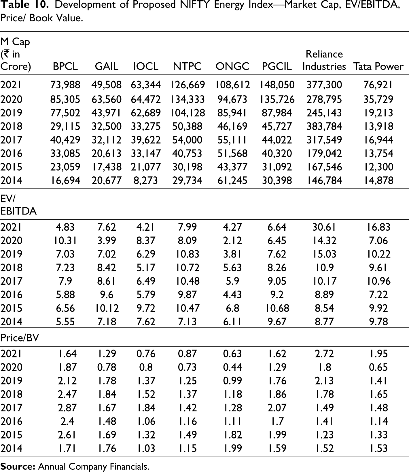
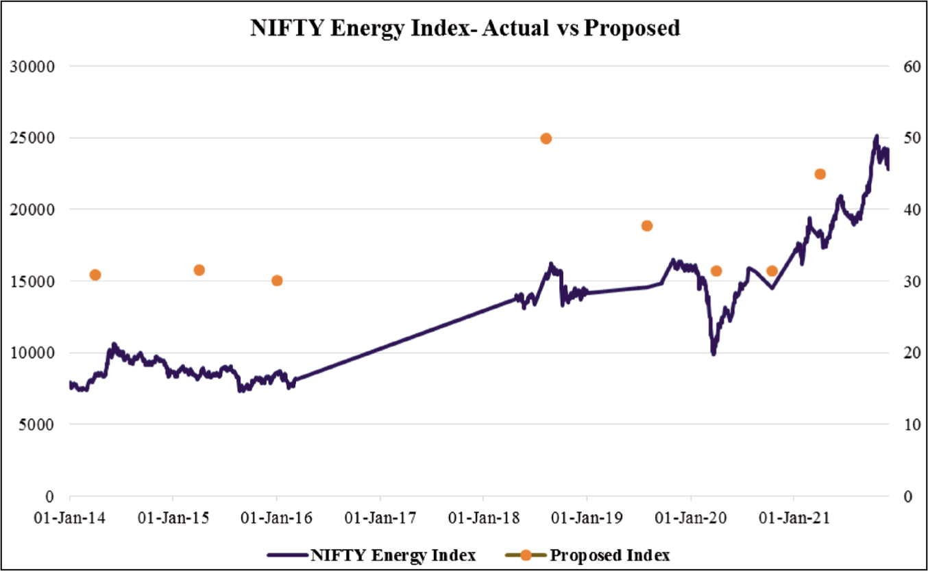
As the empirical analyses significantly rejected both the null hypotheses adopted in Section 3, the study further delved into considering an alternate energy index to relate it with the energy index under consideration or to contribute to future research on proposing a modified and robust Index. This analysis considered the eight stocks, as enumerated in the initial results, which contributed consequentially and sustainably to the sectoral market capitalization for developing an alternate energy index. The market cap value (in crores of Indian rupees), enterprise value/EBITDA ratio, and price/book value ratio have been considered as the key components to devise the index as shown in Table 10. To standardize the variables, the market cap variable has been divided by 10,000 and the price/book value ratio has been multiplied by 10. The weightage of these stocks has been maintained as their market cap proportion to the composite pool of these eight stocks. The individual contribution of these stocks has been evaluated and their weighted addition has been considered to be the new Index since 2014. The index values are shown in Table 11. This research has explicitly reiterated the effectiveness of the NEI for this study, and the same has been verified by comparing the alternate index with the prevailing one. Figure 6 demonstrates the near-similar trajectory of both indices, signifying their correlational movement. Although this study leaves food for thought for an alternate index in the future, it contemplates and reiterates the goodness of the NEI for empirically assessing the hypotheses.

Table 10.

Development of Proposed NIFTY Energy Index—Market Cap, EV/EBITDA, Price/ Book Value

M Cap (₹ in Crore)	BPCL		GAIL	IOCL	NTPC	ONGC	PGCIL	Reliance Industries	Tata Power
2021	73,988		49,508	63,344	126,669	108,612	148,050	377,300	76,921
2020	85,305		63,560	64,472	134,333	94,673	135,726	278,795	35,729
2019	77,502		43,971	62,689	104,128	85,941	87,984	245,143	19,213
2018	29,115		32,500	33,275	50,388	46,169	45,727	383,784	13,918
2017	40,429		32,112	39,622	54,000	55,111	44,022	317,549	16,944
2016	33,085		20,613	33,147	40,753	51,568	40,320	179,042	13,754
2015	23,059		17,438	21,077	30,198	43,377	31,092	167,546	12,300
2014	16,694		20,677	8,273	29,734	61,245	30,398	146,784	14,878
EV/EBITDA
2021	4.83		7.62	4.21	7.99	4.27	6.64	30.61	16.83
2020	10.31		3.99	8.37	8.09	2.12	6.45	14.32	7.06
2019	7.03		7.02	6.29	10.83	3.81	7.62	15.03	10.22
2018	7.23		8.42	5.17	10.72	5.63	8.26	10.9	9.61
2017	7.9		8.61	6.49	10.48	5.9	9.05	10.17	10.96
2016	5.88		9.6	5.79	9.87	4.43	9.2	8.89	7.22
2015	6.56		10.12	9.72	10.47	6.8	10.68	8.54	9.92
2014	5.55		7.18	7.62	7.13	6.11	9.67	8.77	9.78
Price/BV
2021		1.64	1.29	0.76	0.87	0.63	1.62	2.72	1.95
2020		1.87	0.78	0.8	0.73	0.44	1.29	1.8	0.65
2019		2.12	1.78	1.37	1.25	0.99	1.76	2.13	1.41
2018		2.47	1.84	1.52	1.37	1.18	1.86	1.78	1.65
2017		2.87	1.67	1.84	1.42	1.28	2.07	1.49	1.48
2016		2.4	1.48	1.06	1.16	1.11	1.7	1.41	1.14
2015		2.61	1.69	1.32	1.49	1.82	1.99	1.23	1.33
2014		1.71	1.76	1.03	1.15	1.99	1.59	1.52	1.53

Source: Annual Company Financials.

Table 11.

Composite Proposed Energy Index

	BPCL	GAIL	IOCL	NTPC	ONGC	PGCIL	Reliance Industries	Tata Power	Total Index
2021	1.71	1.02	0.93	3.00	1.88	4.50	29.11	2.73	44.88
2020	3.04	1.10	1.40	3.68	1.44	4.24	15.94	0.58	31.42
2019	3.56	1.64	2.10	4.49	2.45	3.82	19.04	0.64	37.74
2018	1.54	1.49	1.20	2.26	1.55	2.18	39.12	0.58	49.92
2017	2.57	1.43	1.79	2.54	2.09	2.35	28.26	0.73	41.77
2016	2.49	1.24	1.48	2.36	2.42	2.77	16.62	0.62	30.01
2015	2.19	1.36	1.43	2.33	3.46	2.85	17.13	0.82	31.57
2014	1.17	1.60	0.45	1.85	5.68	2.51	16.36	1.14	30.76

Source: Annual Company Financials.

Figure 6.

Source: The authors.

VI. Conclusion

The study attempted to verify the dependence of the NEI on crude OP from a long-run time-series perspective. This is because almost two-thirds of the contribution in the NEI is from companies that belong to the industrial production of petroleum goods and are reasonably exposed to the risk of fluctuations in the input prices. Besides this supply-side linkage, the consolidated demand for electricity in the economy instigates for mounting higher IC to meet these increased demands, resulting in an increase in the transactional opportunities for most of the stocks comprising the NEI. Hence, the study also incorporated the argument of the electricity IC to have a possible long-run association with the movement of the NEI. In this multivariate time series analysis, the study offers a thorough econometric analysis of the benchmark energy index in a manner that would fill the research gap in the context of India. From the econometric exercises, the study explored the volatility in the returns of the selected companies with reasonably high market capitalization and found significant short-run and long-run associations among the model variables. The study conducted a dual cointegration analysis and detailed residual analysis to substantiate these results with more robustness. The significant long-run relationship between the NEI, OP and installed electricity generation capacity will provide important insights for proactive policymaking to ensure the non-disruption of the financial market due to supply and demand-side shocks.

After the multivariate analysis, the study proceeds to conduct a univariate econometric exercise to evaluate the predictability of the NEI based on its past values even in the presence of unpredictable exogenous shocks from outside the capital market. The primary reason behind this exercise was to explore the scope for the market players to avoid forthcoming volatility. The study found that India’s benchmark energy index can be effectively prognosticated using an appropriate ARMA model and residual heteroscedasticity EGARCH analysis. Therefore, this prognostication accomplishes better stability and robustness of the entire capital market of India, resulting in the goodness of the broader macroeconomic perspective of the country as well.

The study commands uniqueness in its approach for a three most striking reasons. First, in its multivariate empirical model, it considers a less-explored demand-side impact on the NEI. Second, this study includes the univariate exercise to bring out the expedience of the analysis for forecasting the index. This study is extremely important in establishing non-causality between OP and the energy index, whereas it significantly established bidirectional causality with the electricity IC. This exhorted the importance of policy orientation towards the demand-driven IC to impact not only the financial results of the energy behemoths but also the sustainable growth of the Indian capital market. Third, the study proposed an alternative energy index comprising of financial features of eight consistently contributing companies to the NEI since the last decade. The steadiness of this alternative index and its co-movement with the NEI further substantiates the predictability of the existing index and offers important evidence that exogenous shocks from outside the capital market cannot significantly disturb the prognostication of the NEI.

Footnotes

Declaration of Conflicting Interests

The authors declared no potential conflicts of interest with respect to the research, authorship and/or publication of this article.

Funding

The authors received no financial support for the research, authorship and/or publication of this article.

Notes

References

Ahmad

(2017). An analysis of directional spillover between crude oil prices and stock prices of clean energy and technology companies. Research in International Business and Finance, 42. 10.1016/j.ribaf.2017.07.140

Anbumozhi

, Kalirajan

, & Kimura

(2018). Unlocking the potentials of private financing for accelerated low-carbon energy transition: An overview. In Anbumozhi

, Kalirajan

, & Kimura

(Eds.), Financing for low-carbon energy transition. Springer: 10.1007/978-981-10-8582-6_1

Arago-Manzana

, & Fernandez-Izquierdo

M.A.

(2007). Influence of structural changes in transmission of information between stock markets: A European empirical study. Journal of Multinational Financial Management, 17, 112–124.

Arouri

M.H.

, & Fouquau

(2009). On the short run influence of oil price changes on stock markets in GCC countries: Linear and nonlinear analyses. Economics Bulletin, 29, 806–815.

Arouri

M.E.

, Jouini

, & Nguyen

D.K.

(2011). Volatility spillovers between oil prices and stock sector returns: Implications for portfolio management. Journal of International Money and Finance, 30, 1387–1405.

Arouri

M. E.

, & Rault

(2010). between oil Causal relationships and stock prices: Some new evidence from gulf oil-exporting countries. International Economics, 122, 41–56.

Asteriou

, & Bashmakova

(2013). Assessing the impact of oil returns on emerging stock markets: A panel data approach for ten Central and Eastern European Countries. Energy Economics, 38, 204–211.

Banerjee

(2019). Addressing the drivers of carbon emissions embodied in Indian exports: an index decomposition analysis. Foreign Trade Review, 54(4), 300–333. 10.1177/0015732519874208

Banerjee

(2020). Carbon emissions embodied in India–United Kingdom Trade: A case study on North–South Debate. Foreign Trade Review, 55(2), 199–215. 10.1177/0015732519894149

10.

Banerjee

(2021a). Addressing the carbon emissions embodied in India’s bilateral trade with two eminent Annex-II parties: With input–output and spatial decomposition analysis. Environment Development and Sustainability, 23, 5430–5464. 10.1007/s10668-020-00824-9

11.

Banerjee

(2021b). Carbon adjustment in a consumption-based emission inventory accounting: A CGE analysis and implications for a developing country. Environmental Science and Pollution Research, 28, 19984–20001. 10.1007/s11356-020-11771-3

12.

Banerjee

(2021c). Conjugation of border and domestic carbon adjustment and implications under production and consumption-based accounting of India’s National Emission Inventory: A recursive dynamic CGE analysis. Structural Change and Economic Dynamics, 57, 68–86. 10.1016/j.strueco.2021.01.007

13.

Banerjee

, & Murshed

(2020). Do emissions implied in net export validate the pollution haven conjecture? Analysis of G7 and BRICS countries. International Journal of Sustainable Economy, 12(3), 297–319.

14.

Banerjee

, Hazra

, Khan

M.A.

, & Husnain

M.I.U.

(2021a). Investigating India’s pollution-intensive ‘dirty’ trade specialisation: Analysis with ‘revealed symmetric comparative advantage’ index. Environmental Science and Pollution Research, 28, 30153–30167. 10.1007/s11356-021-12790-4

15.

Banerjee

, Khan

M.A.

, & Husnain

M.I.U.

(2021b). Searching appropriate system boundary for accounting India’s emission inventory for the responsibility to reduce carbon emissions. Journal of Environmental Management, 295. 10.1016/j.jenvman.2021.112907

16.

Batten

, Kinateder

, Szilagyi

, & Wagner

(2017). Can stock market investors hedge energy risk? Evidence from Asia. Energy Economics, 66, 559–570.

17.

Bondia

, Ghosh

, & Kanjilal

(2016). International crude oil prices and the stock prices of clean energy and technology companies: Evidence from non-linear cointegration tests with unknown structural breaks. Energy, 101, 558–565.

18.

Bouri

(2015a). A broadened causality in variance approach to assess the risk dynamics between crude oil prices and the Jordanian stock market. Energy Policy, 85, 271–279.

19.

Bouri

(2015b). Return and volatility linkages between oil prices and the Lebanese stock market in crisis periods. Energy, 89, 365–371

20.

Brockwell

, & Davis

R.A.

(2009). Time series: Theory and methods (2nd ed.). Springer.

21.

Cevik

N.K.

, Cevic

E.I.

, & Dibooglu

(2020). Oil prices, stock market returns and volatility spillovers: Evidence from Turkey. Journal of Policy Modelling, 42(3), 597–614.

22.

Cunado

, & Perez de Gracia

(2014). Oil price shocks and stock market returns: Evidence for some European countries. Energy Economics, 42, 365–377.

23.

da Silva

P.P.

, Moreno

, & Figueiredo

N.C.

(2016). Firm-specific impacts of CO2 prices on the stock market value of the Spanish power industry. Energy Policy, 94, 492–501.

24.

Dutta

(2017a). Oil and energy sector stock markets: An analysis of implied volatility indexes. Journal of Multinational Financial Management, 44, 61–68.

25.

Dutta

(2017b). Oil price uncertainty and clean energy stock returns: New evidence from crude oil volatility index. Journal of Cleaner Production, 164, 1157–1166.

26.

Faff

, & Brailsford

, 1999. Oil price risk and the Australian stock market. Journal of Energy Finance and Development, 4(1), 69–87.

27.

Ferrer

, Shahzad

, Lopez

, Jareño

(2018). Time and frequency dynamics of connectedness between renewable energy stocks and crude oil prices. Energy Economics, 76. 1–20. 10.1016/j.eneco.2018.09.022.

28.

Ghosh

, Sanyal

M.K.

, Jana

R.K.

(2019). Co-movement and dynamic correlation of financial and energy markets: An integrated framework of nonlinear dynamics, wavelet analysis and DCC-GARCH. Computational Economics, 57(1). 10.1007/s10614-019-09965-0

29.

Ghosh

, Sanyal

M.K.

, Jana

R.K.

(2018). An integrated approach incorporating nonlinear dynamics and machine learning for predictive analytics and delving causal interaction. In Bhateja

, Coello

C. A. C.

, Satapathy

S. C.

, & Pattnaiket

P. K.

(Eds.), Intelligent engineering informatics, advances in intelligent systems and computing (pp. 285–300). Springer Nature. 10.1007/978-981-10-7566-7_29

30.

Henriques

, & Sadorsky

(2008). Oil prices and the stock prices of alternative energy companies. Energy Economics, 30, 998–1010.

31.

Jones

, & Kaul

(1996). Oil and the stock markets. The Journal of Finance, 51(2), 463–491.

32.

Kang

, Ratti

R.A.

, & Yoon

(2014). The impact of oil price shocks on U.S. bond market returns. Energy Economics, 44, 248–258.

33.

Kawashima

, & Takeda

(2012). The effect of the Fukushima nuclear accident on stock prices of electric power utilities in Japan. Energy Economics, 34, 2029–2038.

34.

Killian

, & Park

(2009). The impact of oil price shocks on the U.S. stock market. International Economic Review, 50(4), 1267–1287.

35.

Kumar

, Managi

, & Matsuda

(2012). Stock prices of clean energy firms, oil and carbon markets: A vector autoregressive analysis. Energy Economics, 34, 215–226.

36.

Maji

K. I.

(2015). Does clean energy contribute to economic growth? Evidence from Nigeria. Energy Reports, 1, 145–150.

37.

Managi

, & Okimoto

(2013). Does the price of oil interact with clean energy prices in the stock market? Japan and the World Economy, 27, 1–9.

38.

Murshed

, Ali

S.R.

, & Banerjee

(2021). Consumption of liquefied petroleum gas and the EKC hypothesis in South Asia: Evidence from cross-sectionally dependent heterogeneous panel data with structural breaks. Energy, Ecology and Environment, 6(4), 353–377.

39.

Narayan

P. K.

, & Gupta

(2015). Has oil price predicted stock returns for over a century? Energy Economics, 48, 18–23.

40.

Nelson

D.B.

(1991). Conditional heteroskedasticity in asset returns: A new approach. Econometrica, 59, 347–370.

41.

Noor

, & Dutta

(2017). On the relationship between oil and equity markets: Evidence from South Asia. International Journal of Managerial Finance, 13, 287–303.

42.

Oberndorfer

(2009). Energy prices, volatility, and the stock market: Evidence from the Eurozone. Energy Policy, 37, 5787–5795.

43.

Omri

, Mabrouk

N. B.

, Sassi-Tmar

(2015). Modeling the causal linkages between nuclear energy, renewable energy and economic growth in developed and developing countries. Renewable and Sustainable Energy Reviews, 42, 1012–1022.

44.

Rotemberg

J.J.

, & Woodford

(1996). Imperfect competition and the effects of energy price increases on economic activity. Journal of Money, Credit and Banking, 28(4), 549–577.

45.

Sadorsky

(2012). Correlations and volatility spillovers between oil prices and the stock prices of clean energy and technology companies. Energy Economics, 34, 248–255.

46.

Sadorsky

(2014). Modeling volatility and correlations between emerging market stock prices and the prices of copper, oil and wheat. Energy Economics, 43, 72–81.

47.

Salisu

A.A.

, & Isah

(2017). Revisiting the oil price and stock market nexus: A nonlinear panel ARDL approach. Economic Modelling, 66(C), 258–271.

48.

Salisu

A.A.

, & Oloko

T.F.

(2015). Modelling oil price-US stock nexus: A VARMA-BEKKAGARCH approach. Energy Economics, 50, 1–12.

49.

Salisu

A.A.

, Swaray

, & Okolo

T.F.

(2019). Improving the predictability of the oil–US stock nexus: The role of macroeconomic variables. Energy Modelling, 76, 153–171.

50.

Sam

, McNown

, Goh

S.K.

(2019). An augmented autoregressive distributed lag bounds test for cointegration. Economic Modelling, 80(3), 130–141.

51.

Sun

, Ding

, Fang

, Zhang

, Li

(2019). How do fossil energy prices affect the stock prices of new energy companies? Evidence from Divisia energy price index in China’s market. Energy, 169, 637–645.

52.

Swaray

, & Salisu

(2018). A firm-level analysis of the upstream-downstream dichotomy in the oil-stock nexus. Global Finance Journal, 37. 10.1016/j.gfj.2018.05.007.

53.

Ul Husnain

M.I.

, Nasrullah

, Khan

M.A.

, & Banerjee

(2021). Scrutiny of income related drivers of energy poverty: A global perspective. Energy Policy, 157, 112517.

54.

Upadhyay

H.J.

(2019). Examination of Oil Price and its Relationship with Auto Sector and Energy Sector: Case of India. IIMS Journal of Management Science, 10, 141–148. 10.5958/0976-173X.2019.00011.3.

55.

M. T.

(2011). Oil and stock market volatility: A multivariate stochastic volatility perspective. Energy Economics, 33, 956–965.

56.

Vogel

(2010). The significance of residuals for modelling data [Contributed paper]. Eighth International Conference on Teaching Statistics (ICOTS8), July 2010. International Association of Statistical Education (IASE)

57.

Wei

, Qin

, Li

, Zhu

, & Wei

(2019). Oil price fluctuation, stock market and macroeconomic fundamentals: Evidence from China before and after the financial crisis. Finance Research Letters, 30, 23–29.

58.

Wurzburg

, Landeira

, Linares

(2013). Renewable generation and electricity prices: Taking stock and new evidence for Germany and Austria. Energy Economics, 40, 159–171.