Victimization,Crime Propensity,and Deviance: A Multinational Test of General Strain Theory

Abstract

General Strain Theory (GST) identifies victimization as one of the strains most strongly related to crime which, like other sources of strain, is moderated by individual and social factors. Recently, Agnew extended the theorization of coping strategies by proposing that the effects of strain on deviance are conditioned by individual and social factors in combination, rather than singly, which he labeled crime propensity. Tests of the propensity hypothesis have so far yielded mixed results, highlighting the value of additional studies. Whereas previous tests have focused on single countries, either in North America or Asia, we test the propensity hypothesis using data on adolescents in 25 countries collected through the International Self-Report Delinquency Study (ISRD3; n = 57,760). A series of ordinary least squares (OLS) regressions show that the relationship between victimization and delinquency/substance use is conditioned by the effects of individuals’ crime propensity, thereby supporting the recent extension to GST.

Keywords

general strain theory victimization crime propensity ISRD3

Introduction

Even though it may be treated by popular opinion and the law as an incidental irony, criminal behavior subsequent to being victimized has been amply demonstrated in qualitative studies of offenders (e.g., Lockwood, 1997; Luckenbill, 1977; Manasse & Ganem, 2009). For its part, quantitative criminology has revealed the “overlap” between victimization and offending through surveys which show that some individuals report both types of experience during the recent past (Jennings, Piquero, & Reingle, 2012; Posick, 2013; Schreck, Stewart, & Osgood, 2008). The most conservative reading of such results treats the overlap simply as co-occurrence and seeks the causes of this phenomenon in a common underlying factor such as “exposure” to social environments that propitiate both offending and victimization (e.g., Osgood, Wilson, O’Malley, Bachman, & Johnston, 1996) or the personality trait of low self-control (e.g., Higgins, Jennings, Tewksbury, & Gibson, 2009). But there are two theories in criminology—Agnew’s (1992) General Strain Theory (GST) and Wikström’s (2010) Situational Action Theory (SAT)—which offer a causal link between prior victimization and subsequent offending. According to GST, victimization is a “noxious stimulus” (Agnew, 1992, p. 58) which causes strain in the individual and will, with certain coping strategies, lead to criminal behavior as a reaction to that strain. In SAT, victimization represents a source of provocation which, depending upon the characteristics of the person and the setting, can lead to crime as an immediate response. These theories are similar in positing at least some crime as a response to external frictions or provocations and in invoking crime propensity as a key component of the causal process. They differ, among other things, in their center of attention (the person in GST, situations and settings in SAT) and in their conception of crime propensity (multifactorial in GST, morality and self-control in SAT). In this article, we focus on GST, although SAT provides a useful comparator and makes a brief reappearance in our discussion and conclusion.

Although much work has tested GST in relation to varied sources of strain and largely found support for its main propositions (Agnew, 2001), the variables hypothesized as conditioning the link between strain and crime have received only mixed support in empirical studies (Agnew, 2013). This led Agnew (2013) to propose an extension to GST which specified that conditioning variables only play that role when considered in combination rather than singly. However, tests of this extension—most of them including victimization as a source of strain—have also produced mixed results, thereby indicating the need for additional work. In this article, we present a new test of the extension using data from a large multinational sample. We begin with a brief overview of GST and its main concepts and propositions. We then review the prior tests of the extension to GST, noting the varied study designs and mixed results. Following this, we describe the dataset and present our analysis.

GST and the Path From Victimization to Offending

GST has been amply developed and discussed within criminology and the reader is referred to Agnew’s (1992, 2001, 2007, 2013) key publications for a full appreciation of the perspective. In brief, strains are defined as “negative relationships with others” (Agnew, 1992, p. 48) involving failure to achieve valued goals, removal of positively valued stimuli, or exposure to negative stimuli. Victimization is a quintessential strain (Agnew, 1992; Moon, Hays, & Blurton, 2009; Sigfusdottir, Kristjansson, & Agnew, 2012) which can be experienced directly or vicariously and, when perceived as particularly unjust and serious, may lead to subsequent criminal behavior. Agnew (2001) distinguished between “objective strains” (“events or conditions that are disliked by most members of a given group” [p. 320]) and “subjective strains” (“events or conditions that are disliked by the people who are experiencing (or have experienced) them” [p. 321]), both of which play a causal role in subsequent behavior. Victimization can be treated as an objective strain, by measuring its occurrence, and as a subjective strain, by measuring the victim’s evaluation of what happened. According to GST, the link between objective/subjective strain and subsequent offending is mediated by negative emotions, especially anger, which create pressure to adopt corrective actions to alleviate negative feelings. In addition, whether or not individuals respond to victimization (or other sources of strain) with crime depends upon their coping strategies which condition the link between victimization, emotions, and behavioral outcomes. Coping strategies include personal capabilities such as self-efficacy and self-control, social support, social control (e.g., bonding with parents, investment in school), association with (non)criminal peers, and beliefs regarding crime (Agnew, 2013, p. 653). When those coping strategies typify a propensity to crime (i.e., low self-efficacy, low self-control, weak social bonds), offending behavior is more likely to ensue.

Although GST in general and its specific application to the study of the victimization-offending link have received significant empirical support (e.g., Baron, 2009; Hay & Evans, 2006; Kort-Butler, 2010; Manasse & Ganem, 2009; Moon et al., 2009; Turanovic & Pratt, 2013), the proposition regarding the conditional effect of coping strategies has received only mixed empirical support (Agnew, 2013). Some studies have found support for GST in this regard (e.g., Agnew & White, 1992; Baron, 2009; Baron & Hartnagel, 2002; Hay & Evans, 2006; Mazerolle & Maahs, 2000; Turanovic & Pratt, 2013), whereas others have not (e.g., Botchkovar, Tittle, & Antonaccio, 2009; Hoffmann & Miller, 1998; Mazerolle & Piquero, 1997; Paternoster & Mazerolle, 1994). In proposing an extension to GST, Agnew (2013) argued that these varied findings derived from an empirical focus on the separate effects of one or two conditioning variables which measured coping strategies. However, he argued that the effect of any individual conditioning variable is small or modest and it is a combination of coping variables that conditions the response to victimization. Agnew proposed that key coping variables include self-control, social support, association with criminal peers, and beliefs regarding crime. Taken together, these “create a strong propensity for criminal coping” (Agnew, 2013, p. 654). Therefore, a general index measuring the overall crime propensity of individuals is critical to an assessment of its conditional effect on the relationship between strain and crime. It is crime propensity, rather than its individual components, which conditions the link between strain and crime.

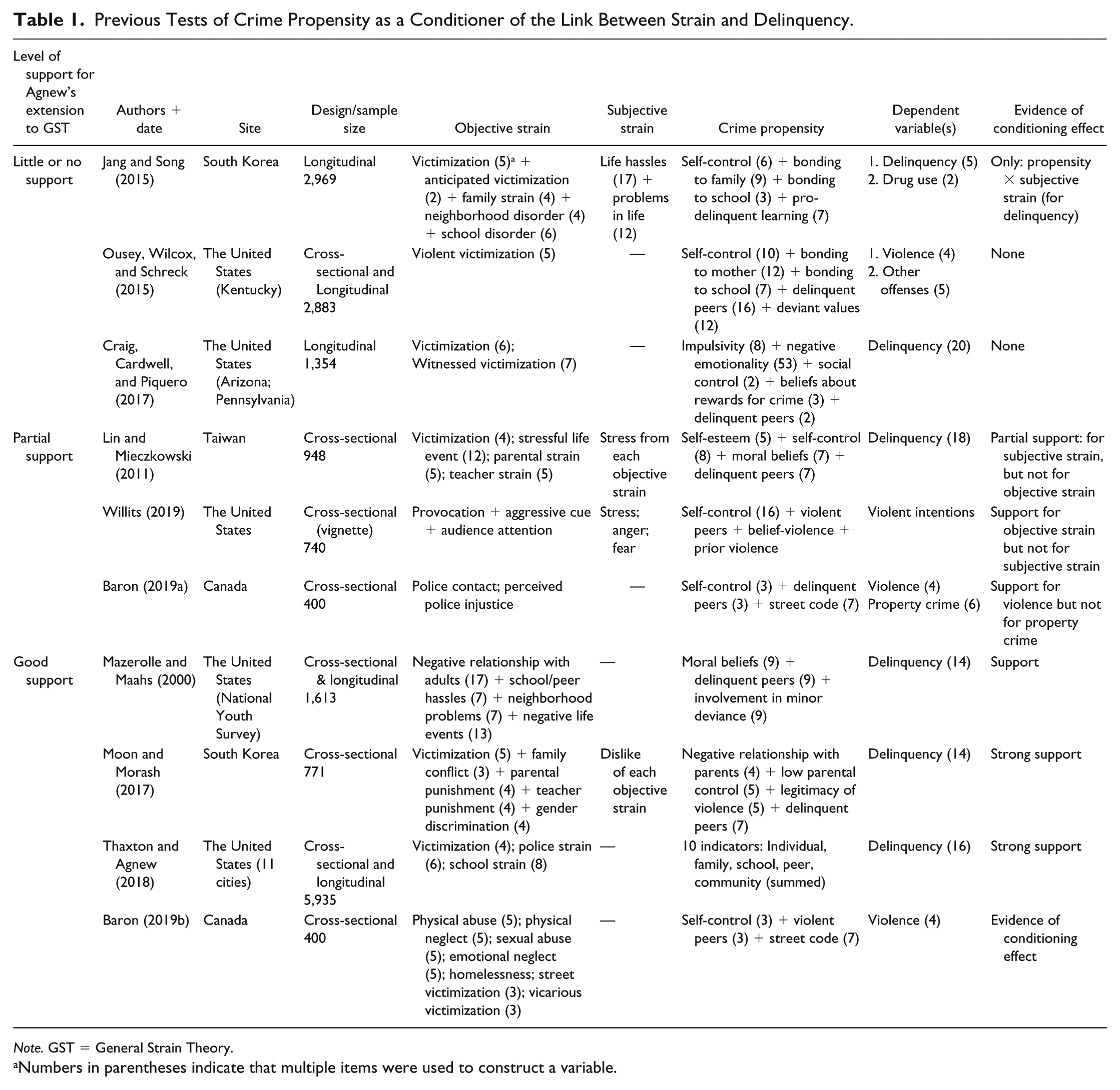
To the best of our knowledge, 10 studies have examined the propensity hypothesis, eight of which have included victimization as a source of strain (see Table 1). Three of these studies (Craig, Cardwell, & Piquero, 2017; Jang & Song, 2015; Ousey, Wilcox, & Schreck, 2015) found little or no support for the hypothesis. For example, Jang and Song (2015) used data from two waves of the Korean Youth Panel Survey. They developed a composite measure of objective strain which combined incidents of victimization, anticipated victimization, family strain, neighborhood disorder and school disorder; and a measure of subjective strain combining levels of stress in relation to common “hassles” (e.g., too much parental control) and the magnitude of common personal problems (e.g., mental health). They also created an index of crime propensity by combining scales for self-control, bonding to family and school, and pro-delinquent learning. The dependent variables were a five-item measure of delinquency and a two-item measure of drug use. The authors found little support for the conditioning effect of propensity on the relationship between strain at Time 1 and crime or drug use at Time 2. Of the four interaction terms they used to examine delinquency (objective strain × delinquent propensity; subjective strain × delinquent propensity; anger × delinquent propensity; depression × delinquent propensity), only subjective strain × delinquent propensity related to crime in the expected direction, whereas none of the interaction terms for propensity was related to drug use.

Table 1.

Previous Tests of Crime Propensity as a Conditioner of the Link Between Strain and Delinquency.

Level of support for Agnew’s extension to GST	Authors + date	Site	Design/sample size	Objective strain	Subjective strain	Crime propensity	Dependent variable(s)	Evidence of conditioning effect
Little or no support	Jang and Song (2015)	South Korea	Longitudinal 2,969	Victimization (5)^a + anticipated victimization (2) + family strain (4) + neighborhood disorder (4) + school disorder (6)	Life hassles (17) + problems in life (12)	Self-control (6) + bonding to family (9) + bonding to school (3) + pro-delinquent learning (7)	1. Delinquency (5) 2. Drug use (2)	Only: propensity × subjective strain (for delinquency)
	Ousey, Wilcox, and Schreck (2015)	The United States (Kentucky)	Cross-sectional and Longitudinal 2,883	Violent victimization (5)	—	Self-control (10) + bonding to mother (12) + bonding to school (7) + delinquent peers (16) + deviant values (12)	1. Violence (4) 2. Other offenses (5)	None
	Craig, Cardwell, and Piquero (2017)	The United States (Arizona; Pennsylvania)	Longitudinal 1,354	Victimization (6); Witnessed victimization (7)	—	Impulsivity (8) + negative emotionality (53) + social control (2) + beliefs about rewards for crime (3) + delinquent peers (2)	Delinquency (20)	None
Partial support	Lin and Mieczkowski (2011)	Taiwan	Cross-sectional 948	Victimization (4); stressful life event (12); parental strain (5); teacher strain (5)	Stress from each objective strain	Self-esteem (5) + self-control (8) + moral beliefs (7) + delinquent peers (7)	Delinquency (18)	Partial support: for subjective strain, but not for objective strain
	Willits (2019)	The United States	Cross-sectional (vignette) 740	Provocation + aggressive cue + audience attention	Stress; anger; fear	Self-control (16) + violent peers + belief-violence + prior violence	Violent intentions	Support for objective strain but not for subjective strain
	Baron (2019a)	Canada	Cross-sectional 400	Police contact; perceived police injustice	—	Self-control (3) + delinquent peers (3) + street code (7)	Violence (4) Property crime (6)	Support for violence but not for property crime
Good support	Mazerolle and Maahs (2000)	The United States (National Youth Survey)	Cross-sectional & longitudinal 1,613	Negative relationship with adults (17) + school/peer hassles (7) + neighborhood problems (7) + negative life events (13)	—	Moral beliefs (9) + delinquent peers (9) + involvement in minor deviance (9)	Delinquency (14)	Support
	Moon and Morash (2017)	South Korea	Cross-sectional 771	Victimization (5) + family conflict (3) + parental punishment (4) + teacher punishment (4) + gender discrimination (4)	Dislike of each objective strain	Negative relationship with parents (4) + low parental control (5) + legitimacy of violence (5) + delinquent peers (7)	Delinquency (14)	Strong support
	Thaxton and Agnew (2018)	The United States (11 cities)	Cross-sectional and longitudinal 5,935	Victimization (4); police strain (6); school strain (8)	—	10 indicators: Individual, family, school, peer, community (summed)	Delinquency (16)	Strong support
	Baron (2019b)	Canada	Cross-sectional 400	Physical abuse (5); physical neglect (5); sexual abuse (5); emotional neglect (5); homelessness; street victimization (3); vicarious victimization (3)	—	Self-control (3) + violent peers (3) + street code (7)	Violence (4)	Evidence of conditioning effect

Note. GST = General Strain Theory.

Numbers in parentheses indicate that multiple items were used to construct a variable.

Three tests of the propensity hypothesis yielded partial support (Baron, 2019a; Lin & Mieczkowski, 2011; Willits, 2019). For example, Willits (2019) used a factorially designed vignette to measure intentions to use violence. Objective strains were written in to the vignette as variations in provocative and aggressive cues from another person and in audience attention to what was happening. Subjective strains measured the respondent’s projected stress, anger, and fear in the scenarios they were presented with. Crime propensity was defined as violent propensity, and operationalized as a combined measure of self-control, beliefs about the use of violence, association with violent criminal peers, and previous use of violence. The dependent variable measured how likely the respondent would be to punch or strike the other person in each scenario. Willits found that violent propensity conditioned the link between objective strains and the intention to use violence, although the relevant interaction term (violent propensity × scenario strain) did not greatly alter the basic pattern and size of the main effects. By contrast, the interaction between violent propensity and subjective strain was not significant.

Four studies found considerable support for the propensity hypothesis (Baron, 2019b; Mazerolle & Maahs, 2000; Moon & Morash, 2017; Thaxton & Agnew, 2018). For example, Thaxton and Agnew (2018) used a large U.S. sample from the project monitoring Gang Resistance Education and Training (GREAT). They developed three separate measures of objective strain: prior victimization, police strain, and school strain. Their measure of crime propensity was the broadest of any used so far to test the conditioning hypothesis, encompassing all major life domains—individual, family, peer, school, and community—and consisting of 10 variables, such as low maternal attachment, poor parental monitoring, impulsivity, risk-taking, low school attachment, criminal neutralizations, and commitment to deviant peers. Their dependent variable was a 16-item scale measuring property offenses, violence, and drug use. Citing a number of problems with statistical models containing interaction terms that assume a normally distributed dependent variable and linear relationships between crime propensity and offending behavior, they employed hurdle models and semiparametric techniques designed to overcome these problems. Their results showed that the conditioning effects of crime propensity are significant and nonlinear, with higher levels of crime propensity significantly increasing the frequency of criminal responses to strain.

As can be seen, the results of these tests of the propensity hypothesis have varied from not supportive through partially supportive to mainly supportive. Table 1 shows that there are numerous variations in study site, sample size and design, and measures of key variables. Much of this variation arises because of the need—which is general in criminology—to rely on datasets that have been designed for a variety of purposes rather than to test a particular theory. However, it also means that thus far, and in relation to tests of the propensity hypothesis, there is no evident pattern of association between a study’s design and its results. For example, the propensity hypothesis has been both confirmed and rejected for: Asian and North American sites, longitudinal and cross-sectional designs, victimization strain, propensity measures including self-control and delinquent peers, and delinquency scales with many or few items. Thus, there is clearly a need to continue testing this hypothesis to accumulate additional results that can contribute to generalizations about its validity and further thought about its specification. The present study is no different to previous ones in that it presents a test of the hypothesis using data from a survey which was not specifically designed to test GST or the propensity hypothesis. However, the sample is markedly different from previous studies because it comprises respondents in 25 countries. Given that theories such as GST claim to be applicable across time and space (Agnew, 2015), this sample offers a unique opportunity to explore the conditionality of the victimization-offending link in a wide variety of societies and cultures. In contrast, previous studies have involved single countries in only two regions of the world: Asia and North America. The next section describes the survey and the measures used to capture key theoretical concepts.

Method

Data

The data are drawn from the International Self-Report Delinquency Study, which has now completed its third sweep (ISRD3; Enzmann et al., 2018). The survey was designed to collect data on the prevalence and incidence of victimization and offending among adolescents, to measure variables of relevance to one or more criminological theories, and to capture key sociodemographic information which is often used as control variables in multivariate modeling of delinquent behavior. As we will see below, it incorporated many of the key variables postulated by GST, including those said to characterize crime propensity. ISRD3 involved the collection of data by national teams using a standard method in each participating country. At the time of the current study, data were available for 25 countries (total n = 57,760) which belong to eight of the world’s cultural groups identified by Inglehart and Baker (2000): African-Islamic, Baltic, Catholic Europe, English-Speaking, Latin America, Orthodox, and Protestant Europe. The average sample size in each country was 2,310 (maximum = 6,430; minimum = 321).¹ Samples were drawn from secondary school students in grades 7 through 9 in a large urban area, one or more additional cities, and sometimes in a wider region. The ISRD samples were not, therefore, representative of all adolescents in each country but of adolescents in urban schools. Classes were randomly selected in each urban area/region included in the study and all students in those classes were invited to participate in the survey. The sample was split almost evenly between female (n = 29,185) and male (n = 28,546) respondents and the ages ranged from 12 to 17 years. To maximize comparability, a standard core questionnaire was used in each participating country, although the mode of delivery varied between online and paper-and-pencil versions.

Measures

Dependent variables

We use two different dependent variables because Agnew (2007) suggested that the causal mechanism linking strain and deviance varies depending upon the conduct analyzed. Some negative emotions, such as anger, should lead to delinquency. By contrast, emotions such as depression or anxiety should lead to substance use, that is, what Agnew (2007) called “passive crimes” (p. 34).

Delinquency

We constructed a 13-item variety scale of self-reported offending during the 12 months prior to the survey. The constituent behaviors were graffiti, damaging property, shoplifting, burglary, bicycle theft, car theft, theft from a car, robbery, theft from a person, carrying a weapon, group fighting, assault (with injury), and drug selling. Each item was scored as 0 = no, and 1 = yes, and the responses to these questions were summed to obtain a variety score ranging from 0 to 13. A higher score reflects more engagement in criminal activity (Kuder–Richardson reliability = .742).²

Substance abuse

We created a six-item variety scale to measure respondents’ use of alcohol and drugs. Respondents were asked to report if they had consumed alcoholic beverages (beer or alcopops, wine, or strong spirits) during the previous 30 days. They were also asked if they had consumed soft (e.g., XTC, speed) or hard drugs (heroin, cocaine, crack) during the previous 12 months. Similar to the delinquency scale, each item was scored as 0 for no substance use, and 1 for each kind of reported use. These dichotomous items were added to create a variety score ranging from 0 to 6. Higher scores indicate more substance use (Kuder–Richardson reliability = .644).

Independent variable: Victimization

The independent variable for GST is strain, in this case victimization. ISRD3 asked about seven types of victimization during the previous 12 months: hate crime, assault, extortion or robbery, theft, cyberbullying, and corporal punishment by parents (two items). We constructed a seven-item variety scale, by scoring 1 for each type of victimization that was reported and 0 when it was not reported (see Craig et al., 2017; Posick & Rocque, 2015; Sweeten, Piquero, & Steinberg, 2013), to give a scale ranging from 0 (no victimization experienced) to 7 (all types of victimization reported). Higher scores indicate a higher level of victimization or strain (Kuder–Richardson reliability = .525).³

Conditioning variables: Crime propensity

Crime propensity is a combined measure of four variables discussed by Agnew (2013).

Criminal peers

We constructed a five-item scale based on respondents’ associations with criminal peers. Respondents were asked whether they had friends who used drugs, shoplifted, or committed burglaries, robberies, or assaults. A score of 1 was given for each of the crimes in which the respondent had a friend involved and 0 if no friend was involved. The scale ranges from 0 to 5 and higher scores indicate greater levels of delinquent behavior among friends (Kuder–Richardson reliability = .655).

Self-control

IRSD3 included a nine-item scale (taken from Grasmick, Tittle, Bursik, & Arneklev, 1993) measuring three dimensions of self-control: impulsivity, risk-taking, and self-centeredness. Respondents were asked how much they agreed with statements such as “I act on the spur of the moment without stopping to think” (impulsivity), “Sometimes I will take a risk just for the fun of it” (risk-taking), and “If things I do upset people, it’s their problem not mine” (self-centeredness). The response categories varied from 1 = “agree fully” to 4 = “disagree fully.” The nine items were entered into an exploratory principal components analysis (Kaiser–Meyer–Olkin [KMO] = .869, p for Bartlett’s test < .001) with the results showing two factors above one unit eigenvalue. However, the second factor barely exceeded the unit value (eigenvalue = 1.091) and was 3 times smaller than the first factor (eigenvalue = 3.954). The first factor explains 44% of the variance, and we therefore use a unidimensional construct of self-control (Cronbach’s α = .838). Responses were coded so that higher values indicate higher self-control.

Beliefs

The scale consists of seven items measuring respondents’ beliefs regarding the wrongness of common crimes or problem behaviors: rebelliousness toward adults, hate speech, vandalism, theft, burglary, assault, and robbery.⁴ Response categories ranged from 1 = “not wrong at all” to 4 = “very wrong.” The seven items were subjected to an exploratory principal components analysis (KMO = .855, p for Bartlett’s test < .001) and formed a single factor with a sole eigenvalue greater than 1 (eigenvalue = 3.612, variance explained = 51.594%). Higher values on this scale (Cronbach’s α = .818) indicate a lower level of beliefs favorable to crime.

Parental supervision

This scale consists of 12 items measuring the extent to which respondents’ activities were controlled or supervised by their parents. Respondents were asked how often, for example, they told their parents who they spent time with, or if their parents knew where they were when they went out. Response categories ranged from 1 = “almost never” to 4 = “almost always.” An exploratory principal components analysis was conducted (KMO = .911, p for Bartlett’s test < .001) and identified three factors above one unit eigenvalue. However, two of them barely overcame the unit value (eigenvalue = 1.185; 1,045) and were around 5 times smaller than the first factor (eigenvalue = 5.094). The first factor explains more than 42% of the variance, and we therefore use a unidimensional construct of parental supervision (Cronbach’s α = .866). Higher values on this scale indicate higher levels of parental supervision.

To create the overall index of crime propensity, first, we standardized the scores for criminal peers. Second, we reversed the scores for the other conditioning variables so that higher scores indicate higher crime propensity. Third, the scores for criminal peers, self-control, beliefs favorable to crime, and parental supervision were added together to form the crime propensity variable (Cronbach’s α = .647).⁵

Control variables

We included the standard demographic variables of age (12-17 years old) and gender (0 = male, 1 = female).

Analytic Plan

First, we conducted a series of ordinary least squares (OLS) regression analyses with two models for each of our dependent variables. As expected, our dependent variables were positively skewed (delinquency skewness = 4.38, substance use skewness = 1.66). However, we logged them to normalize the scales for use in OLS models (delinquency skewness = 1.74, substance use skewness = 0.91). The results did not differ significantly between models with the original and logged values of the dependent variables. Indeed, by and large, the standardized residuals in those models regressing on the original values of our dependent variables are more normally distributed than those with logged dependent variables. In addition, on average, the coefficients $R_{adj}^{2}$ are slightly higher for models with the original values of both delinquency and substance use. Finally, no problems with heteroscedasticity were detected in any of the set of models. Consequently, only the results for the original variables are presented here. In Models 1 and 3, we regress delinquency and substance use, respectively, on victimization, after controlling for the other variables. Second, to determine the impact of the interaction with crime propensity on the relationship between victimization and the dependent variables, we include two additional regression models with interaction terms (Models 2 and 4). We created the interaction term by multiplying the standardized values of victimization and crime propensity (see Aiken, West, & Reno, 1991).⁶

The final set of regression analyses estimated the magnitude of the effect of different levels of individuals’ crime propensity on the relationship between victimization and delinquency/substance use.⁷ To do that, we estimated split-sample models for respondents with low, medium, or high crime propensity. Following other authors’ procedures (see Baron, 2019a; Mazerolle & Maahs, 2000; Serrano-Maíllo, 2018), we divided the sample such that those located at more than one standard deviation below the mean (14% of the sample) were considered low in crime propensity; those located between −1 and +1 standard deviation from the mean (65% of the sample) represented medium crime propensity; and those located more than one standard deviation above the mean (21% of the sample) were high in crime propensity. Finally, to identify significant differences among the coefficients for the three crime propensity clusters for each of our dependent variables, we conducted a series of z tests (Clogg, Petkova, & Haritou, 1995; Paternoster, Brame, Mazerolle, & Piquero, 1998). Table 2 shows the descriptive statistics for all variables included in the models.

Table 2.

Descriptive Statistics for All Variables.

	N	M	SD	Minimum	Maximum
Delinquency	54,318	0.481	1.199	0.000	13.0
Substance use	53,235	0.668	1.076	0.000	6.0
Victimization	55,074	0.762	1.078	0.000	7.0
Crime propensity	51,442	0.0	1.0	−1.672	5.957
Gender	57,731	0.494	—	0.0	1.0
Age	57,760	13.833	1.066	12.0	17.0
Victimization × Crime propensity	49,720	0.086	2.764	−7.376	34.485

Hypotheses

Hypothesis 1 (H1): All else constant, there is a positive relationship between victimization and delinquency/substance use.

Hypothesis 2 (H2): All else constant, victimization leads to higher levels of delinquency/substance use as the level of crime propensity increases.

Results

Table 3 shows the bivariate correlations among all the variables of interest. As is to be expected in samples of this size, all coefficients are significant; thus, it is the size of these coefficients which is of more interest. The analysis shows moderate associations between victimization and delinquency and substance use in the expected direction (.290, .204, at p < .01 level). It also shows strong positive associations between crime propensity and delinquency and substance use (.517, .460, p < .01 level). Given the latter results, multicollinearity could have been an issue affecting modeling. However, Variance Inflation Factors (VIFs) were estimated for each model, and the results did not reveal any variables with a value greater than 1.3 (see Gujarati, 2003). Therefore, multicollinearity is ruled out.

Table 3.

Bivariate Correlations Among Variables.

	1	2	3	4	5	6
1. Delinquency	1
2. Substance use	.395**	1
3. Victimization	.290**	.204**	1
4. Crime propensity	.517**	.460**	.282**	1
5. Gender	.122**	.010*	−.020**	.134**	1
6. Age	.099**	.294**	.034**	.236**	.029**	1

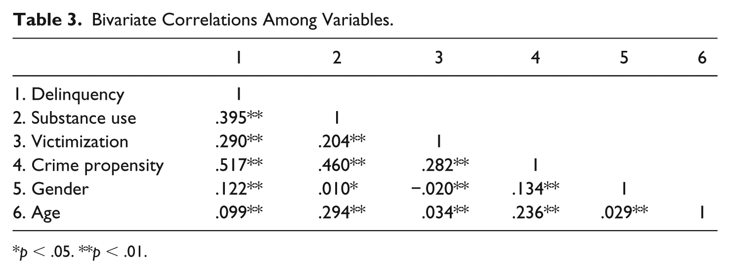
p < .05. **p < .01.

Models 1 and 3, in Table 4, test H1 by estimating the impact of victimization and crime propensity on delinquency and substance use, respectively. Model 1 shows that victimization is positively associated with delinquency after controlling for the other variables, including crime propensity (b = .190, β = .159, p < .001). The model also reveals a strong relationship between the overall index of crime propensity and delinquency (b = .569, β = .468, p < .001). The model fits well and explains more than 29% of the variance, $R_{adj}^{2} = . 294$ , Akaike information criterion (AIC) = 136,395, Bayesian information criterion (BIC) = 136,439. Model 4 shows a similar pattern, although not so strong. There is a positive relationship between victimization and substance use (b = .086, β = .079, p < .001) after controlling for crime propensity (b = .432, β = .395, p < .001) and other variables. Model 4 explains around 26% of the variance ( $R_{adj}^{2} = . 259$ , AIC = 126,662, BIC = 126,706). We can confirm our H1: all else constant, there is a positive relationship between victimization and deviance.

Table 4.

OLS Regression Models Predicting Delinquency and Substance Use.

	Delinquency		Substance use
	Model 1	Model 2	Model 3	Model 4
	b (SE) [β]	b (SE) [β]	b (SE) [β]	b (SE) [β]
Victimization	.190*** (.005) [.159]	.119*** (.005) [.100]	.086*** (.004) [.079]	.069*** (.005) [.064]
Crime propensity	.569*** (.005) [.468]	.530*** (.005) [.435]	.432*** (.005) [.395]	.423*** (.005) [.387]
Gender	.148*** (.009)	.164*** (.009)	−.096*** (.008)	−.092*** (.008)
Age	−.019*** (.004) [−.017]	−.011* (.004) [−.010]	.207*** (.004) [.203]	.209*** (.004) [.205]
Victimization × Crime propensity		.183*** (.004) [.199]		.042*** (.004) [.051]
Constant	.685*** (.062)	.520*** (.060)	−.2,129*** (.058)	−2,166*** (.058)
n	48,021	48,021	47,074	47,074
R ² _adj	.294	.328	.259	.261
AIC	136,395	134,037	126,662	126,522
BIC	136,439	134,090	126,706	126,574

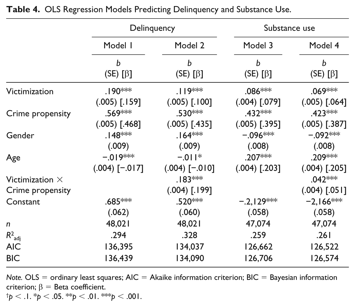
Note. OLS = ordinary least squares; AIC = Akaike information criterion; BIC = Bayesian information criterion; β = Beta coefficient.

†

p < .1. *p < .05. **p < .01. ***p < .001.

To test H2, we introduced the interaction term (victimization × crime propensity) in Models 2 and 4. Model 2 shows a positive relationship between the interaction term and delinquency, net of the effect of the other variables (b = .183, β = .199, p < .001). Results show that the interaction term is statistically significant at p < .001, and the magnitude of the effect is moderately strong (β = .199). In addition, Model 2 shows a better fit than Model 1 ( $R_{adj}^{2} = . 328$ , AIC = 134,037, BIC = 134,090). To assess whether the differences between the coefficients in Models 1 and 2 are statistically significant, we conducted a z test (results not shown). The results confirmed that the coefficients in Model 2 are significantly different from the coefficients in Model 1 at p < .001.

For substance abuse, Model 4 also shows a positive relationship between the interaction term (victimization × crime propensity) and substance use (b = .042, β = .051, p < .001). In addition, the introduction of the interaction term into the equations barely increases the model’s fit ( $R_{adj}^{2} = . 261$ , AIC = 126,522, BIC = 126,574), although it still explains more than 26% of the variance. A z test also indicated that the coefficients in Model 4 are significantly different at p < .01 from the coefficients in Model 3.

These results provide support for H2. There is a positive relationship between the interaction term (victimization × crime propensity) and delinquency, holding victimization and other variables constant. In other words, the frequency of delinquent behavior is significantly higher for victimized individuals with higher levels of crime propensity. For substance use, we find a similar pattern of results: the effect of the interaction term on the link between victimization and substance use is statistically significant after controlling for the other predictors of crime. Thus, substance use is significantly higher at higher levels of association between victimization and crime propensity. The results also show that the model predicting delinquency yields better goodness-of-fit statistics than the model predicting substance use. As such, the data show stronger support for the propensity hypothesis when applied to delinquency as compared with substance use. It is also worth noting that Models 2 and 4 show that the introduction of the interaction term reduces the size of the coefficients for the main effects of victimization and crime propensity (e.g., from β = .159 [Model 1] to β = .100 [Model 2] for victimization and from β = .468 [Model 1] to β = .435 [Model 2] for crime propensity); however, it does not reduce them to negligible values. Overall, Table 4 shows that there is a conditioning effect of crime propensity, but its main effect is still much stronger.

Finally, to reinforce the results found in the previous analysis, we used an additional procedure to test the interactions. Table 5 and Figure 1 present the results of a series of OLS regressions examining the relationship between victimization and delinquency/substance use for three levels of crime propensity. Findings indicate that the association between victimization and delinquency is stronger in the medium crime propensity group (b = .175, β = .215) than in the low propensity group (b = .048, β = .131), and the effects are strongest in the high propensity group (b = .537, β = .324). All the coefficients in Table 5 are significantly different from zero at p < .001. The findings show an identical pattern for substance use, although the differences between propensity groups are not as large as for delinquency. The higher the level of crime propensity, the larger the association between victimization and substance use (low propensity [b = .035, β = .056], medium [b = .113, β = .109], and high [b = .288, β = .250]). All the regression equations show significant relationships between victimization and delinquency/substance use at p < .001. To test whether the coefficients were significantly different between groups, we also conducted a series of z tests (not shown). The results indicated that the coefficients for the low propensity group are significantly different from the coefficients for the medium propensity group, and in turn, these are significantly different from the coefficients for the high propensity group. In addition, all the coefficients are substantially above zero. Figure 1 illustrates the regression lines for the conditioning effect by showing that the slope and intercept in the relationship between victimization and delinquency/substance are higher as the level of individuals’ crime propensity increases.

Table 5.

OLS Regression: The Relationship Between Victimization and Delinquency/Substance Use by Level of Crime Propensity.

Crime propensity	Delinquency			Substance use
	Low	Medium	High	Low	Medium	High
	b (SE) [β]	b (SE) [β]	b (SE) [β]	b (SE) [β]	b (SE) [β]	b (SE) [β]
Victimization	.048*** (.004) [.131]	.175*** (.004) [.215]	.537*** (.015) [.324]	.035*** (.007) [.056]	.113*** (.005) [.109]	.288*** (.011) [.250]
Constant	.066*** (.003)	.322*** (.004)	1.090*** (.019)	.134*** (.006)	.612*** (.005)	1.100*** (.013)
n	7,146	34,249	10,992	7,067	33,438	10,853

Note. OLS = ordinary least squares. β = Beta coefficient.

†

p < .1. *p < .05. **p < .01. ***p < .0005.

Figure 1.

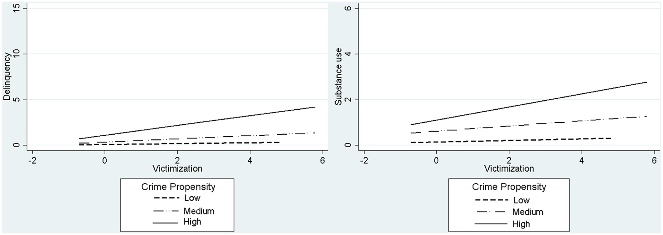
OLS regression lines of victimization predicting delinquency/substance use for three crime propensity groups.

Discussion and Conclusion

Our findings show support for the hypothesized main effect of victimization on delinquency and drug use, and also for the conditioning effect of propensity. In line with prior research (e.g., Baron, 2009; Hay & Evans, 2006; Kort-Butler, 2010; Manasse & Ganem, 2009; Sigfusdottir et al., 2012), our results show that victimization was positively associated with delinquency and substance use when controlling for other predictors of deviance (H1). In relation to H2, our results show that individuals’ crime propensity conditioned the relationship between victimization and deviance, although with varying magnitudes. Thus, the interaction between victimization and crime propensity had a stronger effect on delinquency than on substance abuse. These results therefore represent a fifth study that supports the propensity hypothesis alongside those conducted by Baron (2019b), Mazerolle and Maahs (2000), Moon and Morash (2017), and Thaxton and Agnew (2018). That our findings derive from a large 25-country sample collected in eight of the world’s cultural regions also provides strong support for the generality of the propensity hypothesis, at least in relation to the link between victimization and deviance.

However, it is important to note that this study only provides what Agnew (2013, p. 666) called a “rough” test of the propensity hypothesis (cf. Jang & Song, 2015). More rigorous tests of GST and its extension would require the measurement of several types of objective and subjective strain, of the mediating emotions, and of additional components of propensity. Associated analytical decisions, for example, testing the theory in relation to specific types of victimization and delinquent behavior as opposed to using variety scales, deciding on the constituent elements of composite measures of victimization, propensity and delinquency, and choosing between additive or multiplicative combinations of these elements (see Agnew, 1992), need to be informed where possible by the theory rather than by considerations of method.

An additional limitation of our study lies in its cross-sectional survey design, which does not allow robust inferences about causality. This limitation has been noted in prior studies using a cross-sectional design to test the propensity hypothesis and has been addressed in contrasting ways. On one hand, several authors reporting support for the propensity hypothesis have cited the similarity between the results from tests with cross-sectional and longitudinal designs (Lin & Mieczkowski, 2011; Mazerolle & Maahs, 2000; Thaxton & Agnew, 2018). In their view, this indicates that spurious causal ordering can be ruled out in cross-sectional designs. On the other hand, although they did not find support for the propensity hypothesis, Ousey et al. (2015) argued that the effects of victimization on subsequent deviant behavior are most likely to be short-term such that “situation-specific responses . . . should be more robust in cross-sectional than longitudinal analyses” (p. 172). This is a criticism of the assumption that longitudinal designs are better because it raises the question of the appropriate time lag between victimization as a cause and deviant behavior as an effect. In his initial outline of GST, Agnew (1992) proposed that “recent events are more consequential than older events and that events older than three months have little effect” (p. 65). If this is the case, the longitudinal designs employed in previous tests of the extension to GST have mis-specified the likely time lag between the dependent and independent variables and cannot be considered superior to tests with cross-sectional data. But neither can current cross-sectional survey designs test for causal ordering if they do not measure the temporal ordering of victimization and crime events. Gottfredson and Hirschi (1987) argued that crimes are nontrivial events which can be located quite precisely in time by those who commit them, and we would argue that the same is true for victimization events. They suggested that cross-sectional surveys with retrospective measurement focusing on the previous 6 or 12 months could be designed to capture the temporal sequence of delinquent acts and key causal variables. While not without its own problems, this strategy warrants serious consideration and development, although to our knowledge no such survey has so far been designed.

As noted above, Agnew (2013) argued that existing survey data do not allow rigorous testing of the propensity hypothesis. Indeed, other studies using ISRD data have also found strong associations between the variables herein included and different types of deviant behavior (Manzoni & Schwarzenegger, 2018; Näsi, Aaltonen, & Kivivuori, 2016; Posick & Gould, 2015). These variables can be linked to other theoretical perspectives which also explain the relationship between victimization and delinquency; however, they identify distinct intervening mechanisms (Hay & Evans, 2006). In a similar vein, it is noteworthy that Willits’ test of the propensity hypothesis in GST using a factorially designed vignette does not differ greatly from Wikström, Oberwittler, Treiber, and Hardie’s (2012) test of SAT with a similarly designed vignette. There are, of course, differences between these two theories in the measurement and modeling of key variables, but the overlap is striking. Thus, only more precise specification and testing can fully evaluate the predictive capability of GST’s propensity hypothesis.

Footnotes

Acknowledgements

We are grateful to the ISRD3 Steering Committee, and particularly Dirk Enzmann, for preparing and sharing the data used in this article. We have also benefited greatly from the comments of Alfonso Serrano-Maíllo. We also thank an anonymous reviewer for comments on a previous draft.

Declaration of Conflicting Interests

The author(s) declared no potential conflicts of interest with respect to the research, authorship, and/or publication of this article.

Funding

The author(s) received no financial support for the research, authorship, and/or publication of this article.

Notes

Author Biographies

Marco Teijón-Alcalá is a student on the international doctorate programme at the Universidad Nacional de Educación a Distancia (UNED) in Madrid, Spain, co-supervised by the University of Salford, UK. He has undergraduate degrees in Law and Criminology and a master’s degree in Security. His research interests are: theory testing (especially General Strain Theory), the effects of victimization on criminal behaviour, and quantitative data analysis.

Christopher Birkbeck is professor of Criminology at the University of Salford, UK. Prior to this, he was professsor of Criminology at the Universidad de Los Andes in Venezuela. His current research interests include: testing theories of crime; comparative criminology; and restorative justice.

References

Agnew

(1992). Foundation for a general strain theory of crime and delinquency. Criminology, 30, 47-88.

Agnew

(2001). Building on the foundation of general strain theory: Specifying the types of strain most likely to lead to crime and delinquency. Journal of Research in Crime & Delinquency, 38, 319-361.

Agnew

(2007). Pressured into crime: An overview of general strain theory. New York, NY: Oxford University Press.

Agnew

(2013). When criminal coping is likely: An extension of general strain theory. Deviant Behavior, 34, 653-670.

Agnew

(2015). Using general strain theory to explain crime in Asian societies. Asian Journal of Criminology, 10, 131-147.

Agnew

White

H. R.

(1992). An empirical test of general strain theory. Criminology, 30, 475-500.

Aiken

L. S.

West

S. G.

Reno

R. R.

(1991). Multiple regression: Testing and interpreting interactions. Thousand Oaks, CA: Sage.

Aseltine

R. H.

Jr. Gore

Gordon

(2000). Life stress, anger and anxiety, and delinquency: An empirical test of general strain theory. Journal of Health and Social Behavior, 41, 256-275.

Baron

S. W.

(2009). Street youths’ violent responses to violent personal, vicarious, and anticipated strain. Journal of Criminal Justice, 37, 442-451.

10.

Baron

S. W.

(2019a). Police strain, negative emotions, criminal propensity, and criminal coping. American Journal of Criminal Justice. Advance online publication. doi:10.1007/s12103-019-9471-0

11.

Baron

S. W.

(2019b). Strain, criminal propensity, and violence: Examining the role of the composite moderator in Agnew’s extension to GST. Crime & Delinquency, 65, 801-821.

12.

Baron

S. W.

Hartnagel

T. F.

(2002). Street youth and labor market strain. Journal of Criminal Justice, 30, 519-533.

13.

Botchkovar

E. V.

Tittle

C. R.

Antonaccio

(2009). General strain theory: Additional evidence using cross-cultural data. Criminology, 47, 131-176.

14.

Clogg

C. C.

Petkova

Haritou

(1995). Statistical methods for comparing regression coefficients between models. American Journal of Sociology, 100, 1261-1293.

15.

Craig

J. M.

Cardwell

S. M.

Piquero

A. R.

(2017). The effects of criminal propensity and strain on later offending. Crime & Delinquency, 63, 1655-1681.

16.

Enzmann

Kivivuori

Marshall

I. H.

Steketee

Hough

Killias

(2018). A global perspective on young people as offenders and victims: First results from the ISRD3 Study. Cham, Switzerland: Springer.

17.

Gottfredson

Hirschi

(1987). The methodological adequacy of longitudinal research on crime. Criminology, 25, 581-614.

18.

Grasmick

H. G.

Tittle

C. R.

Bursik

R. J.

Jr. Arneklev

B. J.

(1993). Testing the core empirical implications of Gottfredson and Hirschi’s general theory of crime. Journal of Research in Crime & Delinquency, 30, 5-29.

19.

Gujarati

D. N.

(2003). Basic econometrics. New York, NY: McGraw Hill.

20.

Hay

Evans

M. M.

(2006). Violent victimization and involvement in delinquency: Examining predictions from general strain theory. Journal of Criminal Justice, 34, 261-274.

21.

Higgins

G. E.

Jennings

W. G.

Tewksbury

Gibson

C. L.

(2009). Exploring the link between low self-control and violent victimization trajectories in adolescents. Criminal Justice and Behavior, 36, 1070-1084.

22.

Hirschi

Gottfredson

M. R.

(1995). Control theory and the life-course perspective. Studies on Crime & Crime Prevention, 4, 131-142.

23.

Hoffmann

J. P.

Miller

A. S.

(1998). A latent variable analysis of general strain theory. Journal of Quantitative Criminology, 14, 83-110.

24.

Inglehart

Baker

W. E.

(2000). Modernization, cultural change, and the persistence of traditional values. American Sociological Review, 65, 19-51.

25.

Jang

S. J.

Song

(2015). A “rough test” of a delinquent coping process model of general strain theory. Journal of Criminal Justice, 43, 419-430.

26.

Jennings

W. G.

Piquero

A. R.

Reingle

J. M.

(2012). On the overlap between victimization and offending: A review of the literature. Aggression and Violent Behavior, 17, 16-26.

27.

Kort-Butler

L. A.

(2010). Experienced and vicarious victimization: Do social support and self-esteem prevent delinquent responses? Journal of Criminal Justice, 38, 496-505.

28.

Lin

W. H.

Mieczkowski

(2011). Subjective strains, conditioning factors, and juvenile delinquency: General strain theory in Taiwan. Asian Journal of Criminology, 6, 69-87.

29.

Lockwood

(1997). Violence among middle school and high school students: Analysis and implications for prevention. Washington, DC: National Institute of Justice, Office of Justice Programs, U.S. Department of Justice.

30.

Luckenbill

D. F.

(1977). Criminal homicide as a situated transaction. Social Problems, 25, 176-186.

31.

Manasse

M. E.

Ganem

N. M.

(2009). Victimization as a cause of delinquency: The role of depression and gender. Journal of Criminal Justice, 37, 371-378.

32.

Manzoni

Schwarzenegger

(2018). The influence of earlier parental violence on juvenile delinquency: The role of social bonds, self-control, delinquent peer association and moral values as mediators. European Journal on Criminal Policy and Research. Advance online publication. doi:10.1007/s10610-018-9392-3

33.

Mazerolle

Maahs

(2000). General strain and delinquency: An alternative examination of conditioning influences. Justice Quarterly, 17, 753-778.

34.

Mazerolle

Piquero

A. R.

(1997). Violent responses to situations of strain: A structural examination. Justice Quarterly, 15, 65-91.

35.

Moon

Hays

Blurton

(2009). General strain theory, key strains, and deviance. Journal of Criminal Justice, 37, 98-106.

36.

Moon

Morash

(2017). A test of general strain theory in South Korea: A focus on objective/subjective strains, negative emotions, and composite conditioning factors. Crime & Delinquency, 63, 731-756.

37.

Näsi

Aaltonen

Kivivuori

(2016). Youth hate crime offending: The role of strain, social control and self-control theories. Journal of Scandinavian Studies in Criminology and Crime Prevention, 17, 177-184.

38.

Osgood

D. W.

Wilson

J. K.

O’Malley

P. M.

Bachman

J. G.

Johnston

L. D.

(1996). Routine activities and individual deviant behavior. American Sociological Review, 61, 635-655.

39.

Ousey

G. C.

Wilcox

Schreck

C. J.

(2015). Violent victimization, confluence of risks and the nature of criminal behavior: Testing main and interactive effects from Agnew’s extension of General Strain Theory. Journal of Criminal Justice, 43, 164-173.

40.

Paternoster

Brame

Mazerolle

Piquero

(1998). Using the correct statistical test for the equality of regression coefficients. Criminology, 36, 859-866.

41.

Paternoster

Mazerolle

(1994). General strain theory and delinquency: A replication and extension. Journal of Research in Crime & Delinquency, 31, 235-263.

42.

Posick

(2013). The overlap between offending and victimization among adolescents: Results from the second international self-report delinquency study. Journal of Contemporary Criminal Justice, 29, 106-124.

43.

Posick

Gould

L. A.

(2015). On the general relationship between victimization and offending: Examining cultural contingencies. Journal of Criminal Justice, 43, 195-204.

44.

Posick

Rocque

(2015). Family matters: A cross-national examination of family bonding and victimization. European Journal of Criminology, 12, 51-69.

45.

Schreck

C. J.

Stewart

E. A.

Osgood

D. W.

(2008). A reappraisal of the overlap of violent offenders and victims. Criminology, 46, 871-906.

46.

Serrano-Maíllo

(2018). Crime contemplation and self-control: A test of Situational Action Theory’s hypothesis about their interaction in crime causation. European Journal of Criminology, 15, 93-110.

47.

Sigfusdottir

I. D.

Kristjansson

A. L.

Agnew

(2012). A comparative analysis of general strain theory. Journal of Criminal Justice, 40, 117-127.

48.

Sweeten

(2012). Scaling criminal offending. Journal of Quantitative Criminology, 28, 533-557.

49.

Sweeten

Piquero

A. R.

Steinberg

(2013). Age and the explanation of crime, revisited. Journal of Youth and Adolescence, 42, 921-938.

50.

Thaxton

Agnew

(2018). When criminal coping is likely: An examination of conditioning effects in general strain theory. Journal of Quantitative Criminology, 34, 887-920.

51.

Turanovic

J. J.

Pratt

T. C.

(2013). The consequences of maladaptive coping: Integrating general strain and self-control theories to specify a causal pathway between victimization and offending. Journal of Quantitative Criminology, 29, 321-345.

52.

Wikström

P.-O.

(2010). Explaining crime as moral actions. In Hitlin

Vaisey

(Eds.), Handbook of the sociology of morality (pp. 211-239). New York, NY: Springer.

53.

Wikström

P.-O.

Oberwittler

Treiber

Hardie

(2012). Breaking rules: The social and situational dynamics of young people’s urban crime. Oxford, UK: Oxford University Press.

54.

Willits

(2019). Violent propensity, strain, and violent intentions: A test of Agnew’s revised conditioning hypothesis. Deviant Behavior, 40, 122-137.