Reliability Estimates for Multilevel Designs in Group Research

Abstract

Items that capture group members’ outcomes from small group processes (e.g., satisfaction, cohesion) are often nonindependent. A primary assumption of most measurement models is that the data are independent; applying such models to group-outcome data measured at the individual level of analysis is thus likely to produce inaccurate estimates. A solution to the measurement of nonindependent data involves the use of multilevel modeling to estimate variances at item, individual, and group levels of analysis. Examples from several different statistics programs are provided, and Monte Carlo simulations are used to evaluate the effects of group size and number of items on reliability estimates.

Keywords

reliability estimates multilevel modeling group outcomes

Group processes are related to outcomes at different levels of analysis (Bonito & Hollingshead, 1997). Problems arise, however, when one measures a given individual-level outcome with multiple items because any group member’s true score is not independent from the group to which he or she belongs. Consider, for example, group satisfaction (Keyton, 1991). Individual satisfaction likely varies within and across groups, due in part to differences in the perceived quality of group interaction. Thus, satisfaction within groups is both heterogeneous (based on a set of individual differences) and homogeneous (related to the satisfaction of other members within the group). When data such as these are treated as independent, standard reliability estimates, for example, Cronbach’s (1951) alpha, may provide inaccurate estimates for the scale in question. Thus, one must use different, but by now familiar (at least to most group researchers), methods for assessing individual- and group-level influences on certain types of outcomes, but with a twist that we illustrate below.

We have three purposes in this article. The first is to provide details regarding the estimation of reliability from nonindependent data, focusing specifically on variables that are conceptualized as outcomes of group processes, but are measured at the individual level with multiple items. To illustrate our concerns and to demonstrate an alternative, we limit our discussion to unidimensional constructs, or subconstructs, for which this technique could be used for each dimension. Crucially, we concern ourselves with data collected from groups whose members have interacted with one another prior to measuring the outcome in question and for whom interaction is related to the outcome.¹ These techniques do not apply to, for example, examination of individuals’ satisfaction with groups in general (e.g., Anderson, Martin, & Riddle, 2001). Second, we provide examples of the data structures, syntax, and output for three popular statistical packages: SAS, SPSS, and R. Third, we provide data from Monte Carlo simulations that show the effects of group size, number of items, and interitem correlations on reliability estimates.

The logic underlying many of these issues has been published previously (e.g., Miller & Murdock, 2007; Raudenbush, Rowan, & Kang, 1991), mostly in education research. But group researchers are largely unaware of both the statistical problem and the means by which one generates appropriate estimates with current software packages. In addition, the phenomena of interest to group scholars generally differ from those in education research and can influence estimates of reliability and the inferences drawn from them (as Bonito & Kenny, 2010, have demonstrated in other, relevant areas of group research). The primary difference is the nature of interdependence. In education research, interdependence is often a result of common fate (see Kenny, Kashy, & Cook, 2006); students in a classroom do not generally work toward a common goal (because both the average class size and pedagogical objectives work against it). For groups of the sort that are featured in this journal, interdependence, both in terms of process and outcomes, is a common, often explicit, goal. It follows that interdependence among group members is a characteristic of groups that influences group outcomes as well as individual members’ evaluation of a group’s outcomes or the group processes by which those outcomes were achieved.

It is worth noting at the outset that there are other means to handle such data. For example, one might subtract group means from individual scores and then analyze those deviation scores using techniques that assume independence of observations (e.g., Dineen, Noe, Shaw, Duffy, & Wiethoff, 2007), or one might simply analyze group means for the variables of interest. But doing so is not without cost. When only group means are used as estimates, one is ignoring potentially important variation within groups. And the use of group mean–deviated scores subtracts and ignores the very thing that should be of interest to group researchers, namely, the effect of the group. By pursuing analyses at both the group and individual levels instead, one has a window into both individual functioning within groups and group influences on what individuals say, think, and do (see O’Connor, 2004). It is our hope that researchers and practitioners will employ these methods to gain a better understanding of behavioral phenomena that occur within various types of small groups.

Measurement Reliability

Classical measurement theory is based on the distinction between unobservable or latent constructs and their observable manifest indicators (DeVellis, 1991). Often, but not always, some sort of survey instrument with multiple items is used to assess the construct in question. Keyton (1999), for example, used such an instrument to measure satisfaction with group processes. In other cases, a set of related behaviors might indicate a given construct, such as when group members exhibit power or dominance via interruptions and turn-management (Ng, Brooke, & Dunne, 1995; Smith-Lovin & Brody, 1989). In either case, the items or behaviors are imperfect indicators of the actual magnitude or true score of the construct.

The correlation among multiple items or behaviors serves as a proxy for the relationship between the true score and a given item. The correlations among a set of items are assumed to be caused by the construct they purportedly measure; they function as estimates of association between the true score and the items used to measure it. Of course, the relationship between the true score and its indicators is imperfect and some variance among the items is common and is assumed to be caused by the construct and the remainder is unique to each item. The ratio of the sum of the item variances to the total variation provides the estimate of unique variance, and its complement (subtracting unique variation from one) provides the estimate of common variance. This leads to the familiar equation for Cronbach’s alpha:

α = \frac{k}{k - 1} (1 - \frac{\sum^{​} σ_{i}^{2}}{σ_{y i}^{2}})

The term within parentheses is the common variance of the items, and the ratio of k items to one less than the number of items assures that the range for alpha is between 0 and 1.

The preceding is based on a set of assumptions related to the independence of the items, namely, that item error terms (a) vary randomly, (b) are not correlated with one another, and (c) do not correlate with the true score of the construct in question. For constructs such as the outcomes of group processes, however, such assumptions may not be tenable because manifest indicators covary among group members. It is assumed that such covariation is not coincidental because the outcomes in question share a common antecedent—the coordinated behaviors and verbal contributions to discussion. In short, one’s true score on a given construct depends, in part, on those of his or her colleagues, as evidenced by the intraclass correlations on the manifest indicators.

Generalizability theory (Cronbach, Gleser, Nanda, & Rajaratnam, 1972; Marcoulides, 1996, 2000) provides a window into the problem. Equivalence of measurement is the notion that assessment is relatively consistent across a variety of potentially relevant situations. Equivalence is assumed, for example, if a set of items provides similar assessments across paper and web-based administrations of a survey instrument. However, if mode of administration caused scores to vary, then measurement does not generalize to the universe of all possible types of administrations. The same principle applies to nonindependent data from groups; if a group member’s true score depends, in part, on the group to which a member belongs, then measurement cannot be said to be equivalent across groups.

In fact, several authors have evaluated procedures for estimating the reliability of nonindependent data in other types of designs and have shown how adjustments might be made. For example, Bonito and Kenny (2010) showed how reliability estimates for the social relations model are affected by dyadic- and group-level factors. In addition, Bost (1995) and DeShon, Ployhart, and Sacco (1998) have demonstrated that repeated-measures designs with correlated errors severely bias generalizability estimates when independence is assumed. Because reliability estimates from nonindependent data are informative about both the individual- and group-level processes associated with a construct, it is important to employ appropriate means of calculating such estimates. In the case of single-construct measures from group data, the item-based variance remains the estimate of unique variance, but the covariances represent commonality both within persons and within groups.

In what follows, we describe how to assess reliability for constructs that are assumed to be the outcome of group processes. Our aim is to alert researchers to the problems associated with measurement of nonindependent data, and to provide steps, using several popular software packages, for doing so.

Multilevel Reliability for a Single Construct

The estimation of reliability in the unidimensional case is surprisingly straightforward and is based on concepts familiar to group researchers who have used multilevel techniques. The first step is to compute a version of the so-called unconditional model and then use those estimates to compute reliability estimates at the individual and group levels.

The Unconditional Multilevel Model

Most group and relationship researchers are familiar with the two-level multilevel model (MLM), where individual responses are the first level, and the second level, the group, is the nesting variable. The unconditional model, which does not contain any predictors, is generally the first step in such modeling because it simultaneously identifies variation at the group and individual levels of analysis (Singer, 1998). The model with predictors is called the conditional model. Because computation of reliability estimates for the single-construct case requires only the unconditional model, we will not address the conditional model here. The variance components from the unconditional model are used to estimate the intraclass correlation for the outcome variable, expressed as a percentage. Thus, if 30% of the variation occurs at the group level, then 70% is at the individual level (reported as the residual in most statistical programs). Significance tests are also provided to evaluate whether, for example, group-level variance is significantly different from zero. One then generally adds theoretically relevant predictors at the individual and/or group levels of analysis to explain variation in the outcome variable.

Some statistical notation is warranted. Following Hox (2002), the unconditional model is

Y_{i j} = β_{0 j} + e_{i j}

where

β_{0 j} = γ_{00} + μ_{0 j} .

Here, Y_ij is the score on the outcome measure (for continuous variables) for person i in group j, β_0j is the intercept for group j, γ₀₀ is the grand mean (or the average of all j intercepts), µ_0j is the group effect (or the difference between group j’s intercept and the grand mean, γ₀₀), and e_ij is the error term for person i in group j (which is randomly distributed). As Singer (1998) noted, the unconditional model is simply a one-way random effects ANOVA (analysis of variance) with group as the predictor. The model has two random components, µ_0j and e_ij.The remaining terms are fixed. The MLM decomposes the random components into two variances: $σ_{μ 0}^{2}$ , the variance at the lowest level (in this case, the individual), and $σ_{μ 0}^{2}$ , the variance of the group. The intraclass correlation, which identifies the proportion of variance explained by the nesting variable (again, the group), is computed with the following equation:

ρ = \frac{σ_{μ 0}^{2}}{σ_{μ 0}^{2} + σ_{e}^{2}}

If there is no significant group-level variance, then a researcher could use more common statistical techniques (see O’Connor, 2004, for more on this point).²

MLM Reliability Estimates Based on the Unconditional Model

Multilevel software allows for one dependent variable, but to estimate reliability in the multilevel case we must manipulate the software into working with multiple outcome variables, with group and individual as the predictors. In effect, we need to create a three-level unconditional model, with items nested within individuals who are nested within groups. In this case, all that is needed to estimate the measurement model is one vector containing all the scores from all of the items in the scale, a second vector indicating the participant to whom a given score belongs, and a third vector that identifies the group to which a given participant belongs.³ Item is the lowest level—the error or residual variance $σ_{i t e m}^{2}$ indicates the extent to which items differ within individuals (nested within groups). As Raudenbush and Bryk (2002) have noted, this allows estimation of reliability at the individual and group levels, free from measurement error. The variance $σ_{i n d i v i d u a l}^{2}$ indicates variation in individual means around the group mean on the scale items within groups, and the group-level variation $σ_{g r o u p}^{2}$ indicates variation in the group means on the scale items around the average of the group means.

With the output from a three-level unconditional MLM, one may compute individual- and group-level reliability estimates (see Raudenbush et al., 1991). For the individual-level reliability estimate, the formula is

α_{i} = \frac{σ_{i n d i v i d u a l}^{2}}{σ_{i n d i v i d u a l}^{2} + \frac{σ_{i t e m}^{2}}{p}}

where p is the number of items in the scale. Group-level reliability is estimated with the following formula:

α_{g} = \frac{σ_{g r o u p}^{2}}{σ_{g r o u p}^{2} + \frac{σ_{i n d i v i d u a l}^{2}}{n} + \frac{σ_{i t e m}^{2}}{p * n}}

where n is group size. (In cases where a study includes groups of different sizes, the average group size may be used.) One might define group-level reliability as the homogeneity of means within a cluster or group, but as heterogeneity across groups or clusters. Just as knowing an individual’s mean for the set of items in question allows one to predict his or her score on any given item, knowing the group mean allows for the prediction of an individual’s mean score (as well as his or her item scores) within the group. The group or cluster has some influence on an individual’s response to the item set in question.

Illustration

Data

For illustration, we use data from a study by Park (2008), who examined the effect of socially shared cognition on satisfaction in small groups. Park studied 32 three-person and 35 four-person groups. These groups were composed of different male-to-female ratios. Each group was tasked with assembling an AM radio from a kit; discussion occurred during that task. Participants were asked to respond to the satisfaction items after discussion. The shared cognition manipulation involved giving all members in some groups the same instructions for communicating with other members, whereas members of other groups were given mixed instructions (in a given group, two members were given one set of instructions, and the other members of the group were given a different set).

Park (2008) measured satisfaction using a reduced version of Keyton’s (1991) satisfaction instrument. The original inventory contained 50 items, each of which was categorized as a global satisfier, global dissatisfier, situational satisfier, or situational dissatisfier. Keyton argued that satisfaction is a global construct if discussion progresses as anticipated but becomes more situational when groups fail to deliver what was expected. Park used only the 24 items that measured global satisfiers and of those kept 15, dropping items that related to politeness and efficiency, as well as those that seemed irrelevant to zero-history groups (e.g., “Everyone attends each group meeting”). Confirmatory factor analysis on the remaining 15 items revealed a unidimensional scale, with α = .93. Given the likely nonindependent nature of the data, however, the estimate does not account for group influences on satisfaction. In what follows, we describe how to obtain estimates that account for the nonindependent nature of these data.

Data Structure

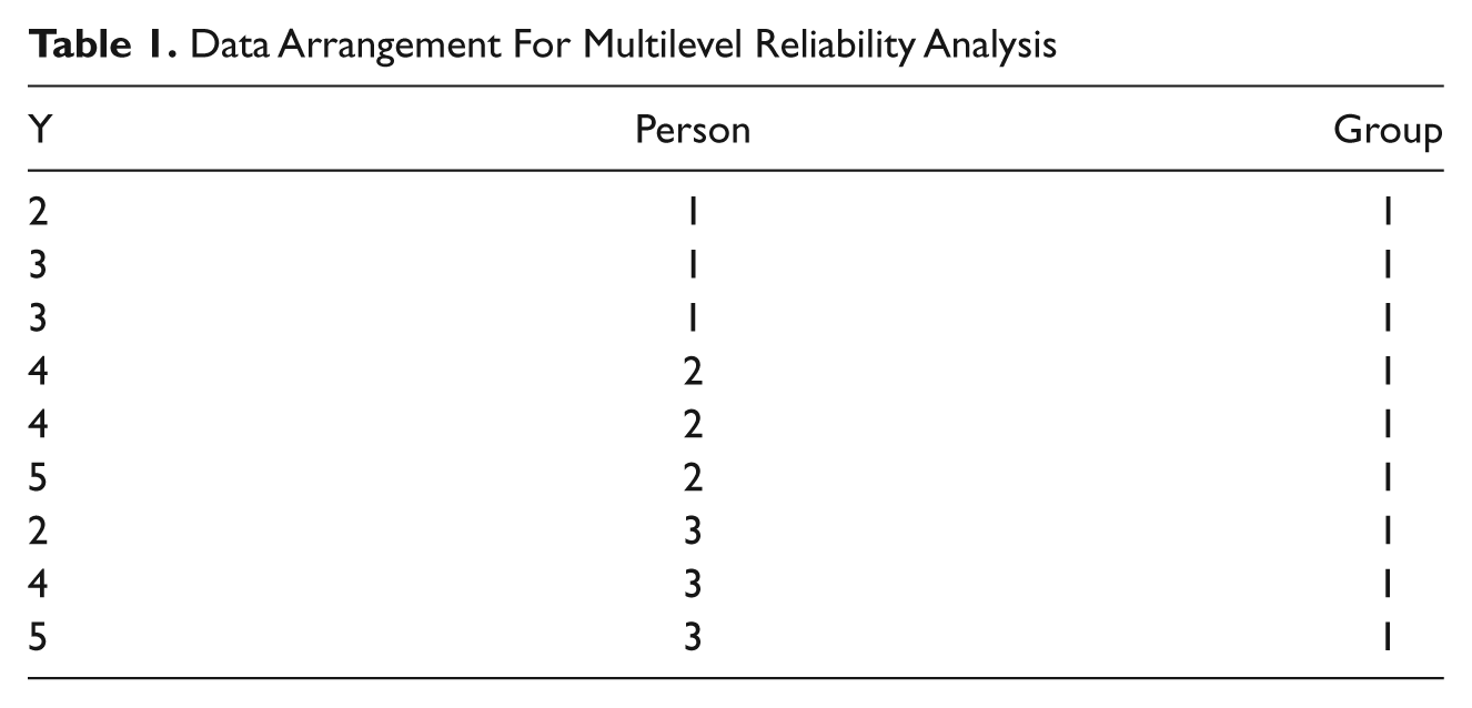
As noted, the basic structure for estimating the reliability of a single construct using the unconditional model is to have a column containing scores for all the items, a column indicating the person who provided the scores, and a column indicating the group to which that person belongs. Space concerns prevent showing the data for all of Park’s 15 items. Instead, as depicted in Table 1, we illustrate how the data were organized using the three-variable case with three-person groups. This can easily be extended to Park’s data by including all 15 scores on the satisfaction items for each participant. The score on the first variable for Person 1 in Group 1 is in the first three columns of the first row, the score for the second variable for that person is in the second row, and so on. Note that each person must have a unique identification number (e.g., the first person in Group 2 would have an ID of 4, and so on).⁴

Table 1.

Data Arrangement For Multilevel Reliability Analysis

Y	Person	Group
2	1	1
3	1	1
3	1	1
4	2	1
4	2	1
5	2	1
2	3	1
4	3	1
5	3	1

Syntax

SAS

PROC MIXED is SAS’s implementation of multilevel modeling and is arguably the most versatile, and most complex, of the three statistical programs discussed here. The syntax for estimating the unconditional model as described above is as follows:

PROC MIXED METHOD=ML COVTEST NOBOUND DATA= DATAFILE;

CLASS GROUP PERSON;

MODEL Y = /SOLUTION DDFM=SATTERTH;

RANDOM INTERCEPT / SUB= PERSON(GROUP) TYPE=UN;

RANDOM INTERCEPT / SUB= GROUP TYPE=UN;

RUN;

Going through each line, “proc mixed” invokes the MLM procedure, “method=ml” specifies maximum likelihood estimation⁵, “covtest” requests statistical tests for each of the variances and covariances estimated, and “nobound” allows the estimation of negative variances when the “random” statement is used.⁶ The “class” statement identifies each of the nesting variables in the design; in this case, items or variables are nested within persons and persons are nested within groups. The “model” statement has the dependent or outcome variable to the left of the equal sign (independent variables go to the right of the equal sign, but the unconditional model does not use them). The “solution” switch tells SAS to print the fixed-effect estimates (which in this case is the intercept), and the DDFM = Satterth requests the Satterthwaite approximation for the degrees of freedom associated with the statistical test for the fixed effects (see Kenny et al., 2006). The first “random” statement (a) indicates the random variable in the design at the person level (intercept), (b) identifies the nesting at the person level (“person(group)”),⁷ and (c) specifies the covariance structure, which is “unstructured.” This covariance structure estimates the variance of the intercept at the individual level. The second “random” statement is identical to the first, except that the nesting variable is the group.

SPSS

Unlike SAS, SPSS has a menu-based interface that allows the user to select a host of procedures with customized output. But SPSS also uses syntax, which, in the interest of space, we will provide here. If the reader would prefer to work with SPSS’s menu options, it should be a relatively simple matter to work from the syntax below to the menu choices available in the Mixed procedure (see Hayes, 2006, for a primer on using SPSS to analyze nested models).

SPSS syntax is similar to that for SAS:

MIXED Y

/FIXED=| SSTYPE(3)

/METHOD=ML

/PRINT=SOLUTION TESTCOV

/RANDOM=INTERCEPT | SUBJECT(SUBJECT) COVTYPE(UN)

/RANDOM=INTERCEPT | SUBJECT(GROUP) COVTYPE(UN).

The first line invokes the “Mixed” procedure, which is SPSS’s implementation of multilevel modeling, and identifies the outcome variable, Y. (Some readers might notice that the “with” statement is missing from the first line, but this is correct, because normally one puts covariates to the right of the “with” statement. The unconditional model does not have covariates.) The “fixed” statement identifies the first level of the three-level unconditional model—there are no fixed predictors, so nothing goes to the right of the equal sign. The “print” statement requests that the parameter estimates and tests for the covariance parameters are included in the output. The remaining lines are comparable to the random statements in SAS.⁸

R

Syntax for the R statistical package (available at http://www.r-project.org/) is much different from that in SAS and SPSS. The basics of R are beyond the scope of this article, and the reader is encouraged to invest the time needed to learn how to read, modify, and write data for that software, as well as to perform basic statistical tests. Two excellent references are Baayen (2008) and Faraway (2006). The syntax for R to estimate an unconditional model is as follows:

MODEL1<-LMER(Y ~ 1 + (1|PERSON) + (1|GROUP), DATAFILE, REML=FALSE)

SUMMARY(MODEL1)

The statement begins with an arbitrary model name to the left of the “<-” symbol—here we use “model1,” but any useful name will do. It is important to note, however, that R uses this name when referencing estimates associated with the model that are stored in memory. The “lmer” statement is R’s MLM implementation and is extensively discussed by Baayen (2008) and Bliese (2009).⁹ The model statement begins with the first open parenthesis, which is followed by the name for the column that contains the dependent variable (“Y,” in this case). The tilde (~) that follows is akin to the equal sign used by both SAS and SPSS, and the 1 immediately following the tilde includes the intercept in the model. (The default in R is to estimate the intercept. One may use “-1” to omit that estimate when needed.) The second open parenthesis contains the random effects at the individual level, which in this case is the variance associated with the intercept. The first closed parenthesis ends the individual-level specification. The next open parenthesis contains the group-level random effects and is identical to the statement for individuals (except, of course, the nesting variable). It ends with another closed parenthesis. The name of the data file (which for illustration is called “datafile” here), the estimation method “REML=FALSE” (which tells R to use maximum likelihood), and a closed parenthesis end the syntax. (It is important to note that R defaults to the unstructured covariance matrix and automatically computes the estimates of the random variances). Finally, the “summary” statement prints the results of the “lmer” procedure in the previous line.

Output

SAS

Relevant SAS output (excluding, for example, iteration history) is in Table 2. The intercept (the grand mean) is 5.27 on a scale of 7—see the “Fixed Effect Estimates” portion of the table. The column labeled “Cov Parm” provides two important pieces of information. The first is the abbreviation for the covariance structure used in the analysis (“UN” for “unstructured”), and the second is the matrix position for the variables in the analysis. Thus, “UN(1, 1)” is the first-row and first-column position for the first variable (the intercept) in the variance–covariance matrix. Because there is only one variable, the matrix consists of just one value, and because the row and column markers are the same, the estimate is a variance. In more complicated designs, one may have several random variances and covariances. The column “Subject” identifies the level of analysis, which in this case indicates that we have two intercept variances, one at the individual and the other at the group level of analysis. The “Estimate” column provides the value for the variance or covariance in question, and the remaining columns provide information regarding the statistical test for the null hypothesis that a parameter is zero in the population.

Table 2.

SAS Output for Park’s (2008) 15-Item Satisfaction Scale

		Covariance Parameter Estimates
Cov Parm	Subject	Estimate	Standard Error	z Value	Pr z
UN(1,1)	SUBJECT (GROUP)	0.5222	0.06508	8.02	<.0001
UN(1,1)	GROUP	0.3744	0.09558	3.92	<.0001
Residual		1.0976	0.02725	40.28	<.0001

		Solution for Fixed Effects
Effect	Estimate	Standard Error	df	t Value	Pr > \|t\|

Intercept	5.2683	0.09097	67.3	57.91	<.0001

SPSS

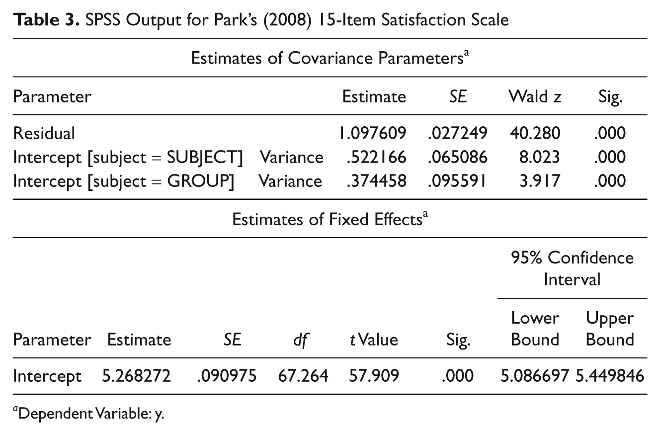
Output from the SPSS mixed procedure is reported in Table 3. Note that the output format differs from that used in SAS, but the estimates are virtually identical. In this case, the residual appears first in the table, the variance estimate for the individual-level analysis is next, and the group-level variance is last.

Table 3.

SPSS Output for Park’s (2008) 15-Item Satisfaction Scale

Estimates of Covariance Parameters^a
Parameter				Estimate	SE	Wald z	Sig.
Residual				1.097609	.027249	40.280	.000
Intercept [subject = SUBJECT] Variance				.522166	.065086	8.023	.000
Intercept [subject = GROUP] Variance				.374458	.095591	3.917	.000

Estimates of Fixed Effects^a
						95% Confidence Interval
Parameter	Estimate	SE	df	t Value	Sig.	Lower Bound	Upper Bound

Intercept	5.268272	.090975	67.264	57.909	.000	5.086697	5.449846

Dependent Variable: y.

R

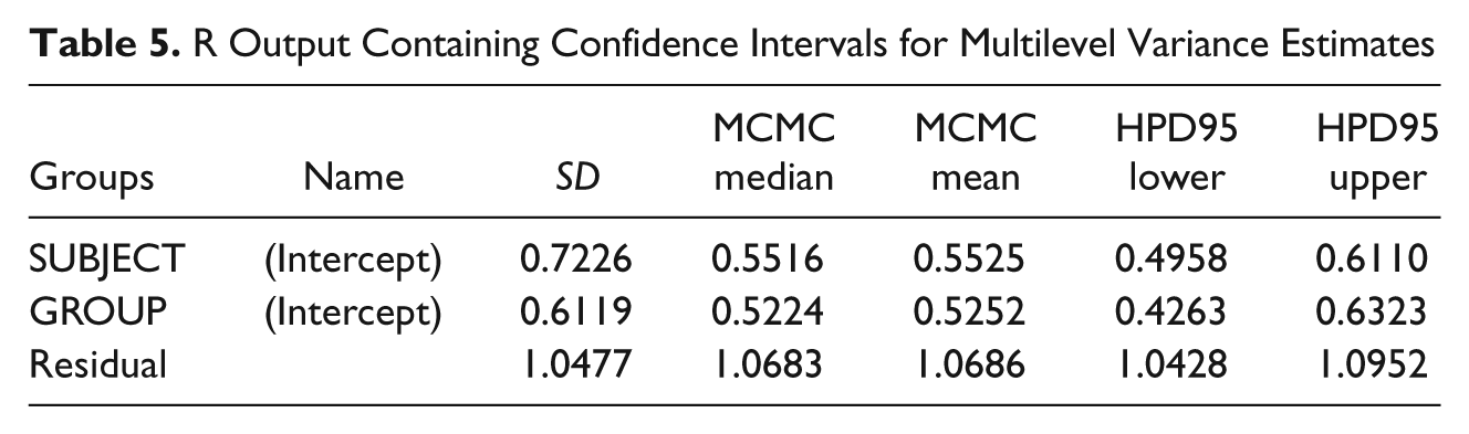
Output from R is presented in Table 4. Notice that the “summary” command (with the model name in parenthesis) was used to display model estimates that were computed by the lme4 procedure. The estimates are comparable to those produced by SAS and SPSS. An interesting issue regarding R multilevel output is the absence of significance tests. This is by design, because the R community treats such tests as flawed for these estimates and prefers Monte Carlo simulations to estimate confidence intervals (Baayen, Davidson, & Bates, 2008). Following Bayeen et al., the parameter estimates and confidence intervals for Park’s data are presented in Table 5.¹⁰ The two rightmost columns contain the lower and upper bounds, respectively, for the confidence interval. Because variances are positive, and are never zero, the confidence interval will never contain zero. Estimates whose lower bounds approach zero should be treated with caution.

Table 4.

R Output for Park’s (2008) 15-Item Satisfaction Scale Random effects

Groups	Name	Variance	SD
SUBJECT	(Intercept)	0.52217	0.72261
GROUP	(Intercept)	0.37446	0.61193
Residual		1.09761	1.04767

Table 5.

R Output Containing Confidence Intervals for Multilevel Variance Estimates

Groups	Name	SD	MCMC median	MCMC mean	HPD95 lower	HPD95 upper
SUBJECT	(Intercept)	0.7226	0.5516	0.5525	0.4958	0.6110
GROUP	(Intercept)	0.6119	0.5224	0.5252	0.4263	0.6323
Residual		1.0477	1.0683	1.0686	1.0428	1.0952

Computing the Multilevel Reliability Estimates

Output from any of the three software packages may be used to calculate reliability for Park’s data using formulas 5 and 6.¹¹ Because group size is variable, the average of group size, approximately 3.5, was used. The number of items was 15. Individual-level reliability was estimated as .88, whereas group-level reliability was .69. These data still exhibit acceptable, by conventional standards,¹² reliability at the individual level, but the estimate is somewhat smaller than the estimate (.93) computed when the data were assumed to be independent. The group-level reliability of .69 indicates that the average of the scores within a group cluster around the group mean and that group means differ from one another. Thus, the group mean for a variable can be a relatively accurate predictor of the mean scores within the group on that variable. This is analogous to the information provided by acceptable individual-level reliability; that is, an individual’s score on a given item can be predicted from that individual’s mean score with relative accuracy. Thus, knowing the group to which a person belongs helps to estimate that person’s true score, at least in this case.

Simulation Studies

In this section, we provide the results of Monte Carlo simulations for the estimation of multilevel reliability. Individual- and group-level reliability (as shown in Formulas 5 and 6) differ slightly in terms of the components used in their estimation. Reliability at the individual level increases with the number of items and the correlation among items, whereas group size, the number of items, the correlation among items, and the homogeneity of scores of individuals within groups (i.e., intraclass correlation) influence group-level reliability (see Raudenbush et al., 1991, for computational details). Not evident in the formulas, but an inherent feature of MLM designs, is the separation of the variances at the three levels of analysis. Thus, the individual-level reliability estimate does not contain variance due to groups, which is preferred, and the group-level estimate accounts for individual variance in the numerator as part of the overall variance (controlling for group size). It is not clear, however, how the three levels of variance (item, individual, and group) interact to affect estimates. Thus, the general thrust of our simulations is to investigate the effects of group size, average item correlation, and number of scale items on the distribution of estimates that reach or exceed the conventionally accepted threshold of .70 for individual-level, nonindependent assessments of reliability.

Our simulations were based on our analysis of Park’s (2008) data. We used a grand mean of 5 (which is close to what Park observed) and set the group deviations from the grand mean to be randomly and normally distributed with variance = 1.00. Our approach was to generate a true score for each individual based on these estimates and then use that true score as the basis for each person’s item score (DeVellis, 1991).¹³ This kept the item means and variances roughly similar but allowed the scores to vary within individuals (nested within groups). The average of the item correlations for Park’s data was approximately .50, but we varied the correlations using a range (.30-.80) that we reasoned was typical of self-report data—smaller correlations are typically not significant and larger ones are fairly rare. We used 1,000 simulations per run. Finally, we examined group sizes of 2, 4, and 6.¹⁴

Table 6 contains the output from the simulations. Our primary concern is the difference between raw (unadjusted) and individual-level (adjusted according to Formula 5) reliability estimates, but we also report group-level reliability estimates because they provide an estimate of the extent to which the group figures into the individual-level estimates. The results show that raw alpha is relatively larger than adjusted individual alpha, and the difference persists across group size and number of items for low interitem correlations. The differences decrease, however, as the interitem correlations increase. For a five-item scale, interitem reliability must be relatively high, above .70, in order for individual-level reliability to reach conventionally adequate levels. Using 10 items, however, requires an interitem correlation of only .50 for adequate reliability. In general, for estimates of individual-level reliability, group size does not matter nearly as much as does the number of correlated items.

Table 6.

SAS Output From Simulations Based On Park’s (2008) Data

	Number of Items = 5
	n = 2			n = 4			n = 6
Correlation	Raw	Individual	Group	Raw	Individual	Group	Raw	Individual	Group
.30	0.46 (0.09)	0.26 (0.16)	0.38 (0.17)	0.48 (0.06)	0.32 (0.09)	0.53 (0.11)	0.48 (0.06)	0.32 (0.07)	0.63 (0.09)
.40	0.61 (0.06)	0.42 (0.11)	0.46 (0.15)	0.62 (0.04)	0.45 (0.06)	0.64 (0.08)	0.62 (0.04)	0.46 (0.05)	0.71 (0.06)
.50	0.72 (0.04)	0.56 (0.10)	0.5 (0.16)	0.72 (0.04)	0.56 (0.06)	0.67 (0.09)	0.72 (0.03)	0.56 (0.05)	0.76 (0.06)
.60	0.78 (0.04)	0.63 (0.08)	0.53 (0.13)	0.79 (0.02)	0.66 (0.04)	0.71 (0.07)	0.79 (0.02)	0.65 (0.03)	0.79 (0.05)
.70	0.84 (0.03)	0.70 (0.07)	0.58 (0.12)	0.84 (0.02)	0.72 (0.03)	0.73 (0.07)	0.84 (0.02)	0.72 (0.03)	0.80 (0.04)
.80	0.87 (0.02)	0.78 (0.04)	0.57 (0.12)	0.87 (0.02)	0.78 (0.03)	0.74 (0.06)	0.87 (0.02)	0.77 (0.02)	0.80 (0.05)

	Number of Items = 10
	n = 2			n = 4			n = 6
Correlation	Raw	Individual	Group	Raw	Individual	Group	Raw	Individual	Group

.30	0.65 (0.05)	0.49 (0.11)	0.44 (0.17)	0.64 (0.04)	0.47 (0.06)	0.63 (0.09)	0.64 (0.04)	0.48 (0.05)	0.72 (0.07)
.40	0.76 (0.04)	0.61 (0.08)	0.52 (0.13)	0.77 (0.03)	0.63 (0.05)	0.69 (0.08)	0.77 (0.02)	0.62 (0.04)	0.78 (0.05)
.50	0.83 (0.03)	0.71 (0.06)	0.57 (0.12)	0.84 (0.02)	0.72 (0.03)	0.73 (0.07)	0.84 (0.02)	0.72 (0.03)	0.80 (0.05)
.60	0.88 (0.02)	0.79 (0.04)	0.58 (0.10)	0.88 (0.01)	0.79 (0.02)	0.75 (0.05)	0.88 (0.01)	0.79 (0.02)	0.82 (0.04)
.70	0.91 (0.01)	0.83 (0.03)	0.60 (0.09)	0.91 (0.01)	0.84 (0.02)	0.74 (0.07)	0.91 (0.01)	0.84 (0.02)	0.82 (0.04)
.80	0.93 (0.01)	0.87 (0.03)	0.61 (0.09)	0.93 (0.01)	0.87 (0.02)	0.76 (0.05)	0.93 (0.01)	0.87 (0.01)	0.83 (0.04)

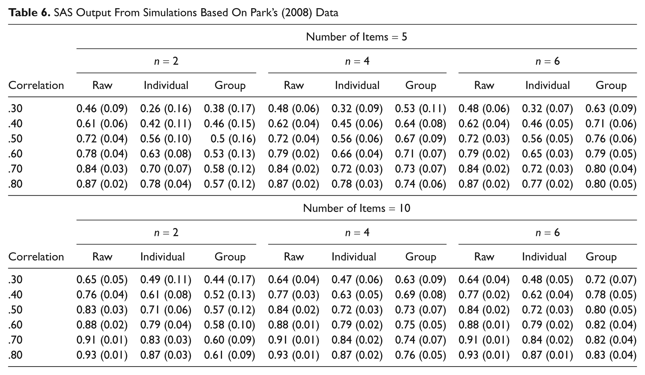
It is instructive to examine how varying group size and the item correlations affects group-level reliability because group-level reliability (a) figures prominently in the estimation of individual-level reliability, and (b) is of potential interest in its own right. The larger the group, the greater the group-level alpha. For six-person groups, a moderate to small correlation among items provides acceptable group-level reliability estimates in both 5- and 10-item scales. In contrast, for two-person groups, a large interitem correlation of .80 and 10 items is not sufficient to increase group-level alpha above .70. This trend follows other features of multilevel designs, for example, that power to detect significant differences rests on larger cluster sizes but not necessarily more clusters (e.g., Hox, 2002).

Discussion

Conceptual and Practical Issues

Scale reliability estimation using MLM relies on a three-level model, with scale items nested within individuals and individuals nested within groups. Implementation of MLM for reliability estimation allows researchers to answer questions about correlations among scale items at multiple levels of analysis. Our goal was to demonstrate the application of MLM to the computation of correlations and reliability estimates in multilevel data using three popular statistics packages and to report on the effects of number of groups, group size, average item correlation, and number of scale items on reliability estimates with nonindependent data. We provided an example of applying the MLM to the computation of individual- and group-level Cronbach’s reliability estimates and Monte Carlo simulation regarding the effects of group size, average item correlation, and number of scale items on reliability estimates at the group and individual levels.

In our example of reliability estimation using Park’s (2008) study of group satisfaction, Keyton’s (1991) global satisfier scale displayed internal consistency at the individual level but not at the group level. Furthermore, the individual-level reliability estimate was slightly inflated when nonindependence was ignored. As the results of our example suggest, accounting for the multilevel nature of group data when examining correlations and reliability is important to the appropriate conceptualization of both observed effects and the variables on which those effects are based. Failing to account for group membership confounds group- and individual-level effects, producing an estimate that might not be representative of either.

Although the statistical benefits of an appropriate analysis of the correlations and reliabilities in nonindependent data are clear, the conceptual implications of such analyses are less straightforward. For example, it is not clear what to do with scales that lack sufficient reliability at the individual level, but exceed conventional thresholds of reliability at the group level, or vice versa. Statistically, we know that poor reliability increases the standard error for statistical tests, so it makes sense to refine the instrument rather than go ahead with tests based on unreliable (and, by extension, not valid) scales.

Furthermore, it would be helpful to know which aspects of group process account for variation at the group level of analysis. Consider, for example, the case of participation in small groups (e.g., Bonito & Hollingshead, 1997). It is possible that groups with higher mean participation rates have higher (or lower) means on the outcome measure of interest (e.g., satisfaction), which obviously contributes to variation in that outcome measure at the group level. The principle is similar for the effect of the group on reliability estimates and is analogous to how generalizability theory (Cronbach et al., 1972; Marcoulides, 2000) evaluates the contributions of testing context to the variability of the items in question. In both cases, the goal is to identify and isolate sources of variance to better understand internal consistency.

The preceding is not limited to the unidimensional case. Although not discussed here, the techniques for assessing reliability for the unidimensional case can be extended (with difficulty) to constructs with multidimensional features. The basics for developing covariance matrices at multiple levels are found in Hox (2002) and Gonzalez and Griffin (2002). Also problematic is the fact that measurement models may fit the data at one level of analysis but not at others. Hollenbeck and associates (Hollenbeck, Ilgen, LePine, Colquitt, & Hedlund, 1998; Hollenbeck et al., 1995), for example, have argued for multilevel model of decision making, in which factors at the individual, dyadic, and group levels influence (or at least account for significant amounts of variance in) decision making. It is not yet clear how measurement issues should be addressed at multiple levels, but any theory or model of group processes that makes claims at multiple levels should consider how measurement may work at one level but not at others (see also Bonito & Kenny, 2010, on this point).

The Importance of Evaluating Outcomes Associated With Group Process

As some psychologists have noted, there is a research trend away from the direct observation of people working together (e.g., “people talking to one another”; Moreland, Fetterman, Flagg, & Swanenburg, 2010, p. 28) to the study of less social activities (e.g., self- or other-ratings), using social cognition as a research foundation. Thus, in psychology, process is anchored at the individual and internal level rather than at the group and observable level. The examination of individual- and group-level outcomes is similarly anchored in internal rather than in social and communication processes (see Hewes, 1996, 2009, for more on this point). Our analysis of Park’s satisfaction data shows, however, that even something that is putatively an internal, individual-level process is also imbued with group-level influences.

Throughout this article, we have acknowledged our preference for evaluating outcomes associated with group processes. More specifically, as communication scholars we argue that group processes (i.e., interactions among group members) are the primary influence on group outcomes. Moreover, we posit that what happens is communication among group members and that such communication will account for the interdependence of group members’ perceptions. A group’s outcomes are a direct result of all members’ interactions. Although reliability estimates of individual group members’ perceptions may be useful if individual rather than group outcomes are evaluated, the presence of group outcomes in a research design, especially when process variables are outcome measures, requires a different approach. Pavitt (1993) cleverly directed readers through different configurations of the role that communication can play in group decision making. He argued that “process is related to outcome variables independent of the impact of relevant input variables on that outcome” (p. 224) and that any change that occurs in a group (e.g., from pre- to post-discussion preferences) “implies that we must consider communication for an adequate explanation of the decision-making process” (p. 225). And as with many processes, communication can influence more than group decision making. For example, communication can also influence cognitive change at the individual level and relationship development among group members. As demonstrated in this article, however, that influence will vary for members within and across groups. We posit that only by estimating reliabilities at both individual and group level will group researchers better understand group process.

If group process (and hence, communication) does not matter, then why do communities and societies rely on groups to problem solve at work, create laws, adjudicate guilt or innocence, nurture children, entertain, socialize, or worship? Even in groups or teams that have more physical than cognitive tasks (e.g., soccer team vs. decision-making group), verbal and nonverbal communication as a process matters. If not, then how could team players signal to one another to change their strategy for making a goal while playing the game? Moreover, the influence of communication (or any process) among group members is not universal in causing within-group variation. Thus, we argue that group process, especially group members’ interactions, drives variation in group outcomes (e.g., satisfaction) and outputs (e.g., winning). Teams do not exist without members and the interactions among them. Thus, the inherent nesting of individuals in groups and teams requires that researchers account for group membership when assessing the reliability of outcome variables.

Conclusion

Although use of the MLM is not without complications and complexities remain regarding the interpretation of the resulting reliability estimates, the ability to examine those estimates at multiple levels of analysis allows for the use of theories and investigation of effects in which individual- and group-level processes are distinguished. This type of analysis can be applied not only to groups but also to dyads, families, organizations, and any other type of data in which some nesting variable serves to group individuals. We hope that the examples we have provided will allow team and group researchers interested in examining the influence of group process to more easily implement the MLM in relevant investigations.

Footnotes

Declaration of Conflicting Interests

The author(s) declared no potential conflicts of interest with respect to the research, authorship, and/or publication of this article.

Funding

The author(s) received no financial support for the research, authorship, and/or publication of this article.

Notes

Bios

Joseph A. Bonito (PhD, University of Illinois at Urbana–Champaign) is associate professor of communication at the University of Arizona. His research interests include group communication, decision making, and methodological issues related to nested data structures.

Erin K. Ruppel (PhD, University of Arizona) is an assistant professor in the Department of Communication at SUNY College at Brockport. She studies communication technologies, health information seeking, and interpersonal communication.

Joann Keyton (PhD, The Ohio State University) is professor of communication at North Carolina State University. Her group scholarship focuses on relational communication, collaboration, and team science.

References

Anderson

C. M.

Martin

M. M.

Riddle

B. L.

(2001). Small Group Relational Satisfaction Scale: Development, reliability and validity. Communication Studies, 52, 220-233. doi:10.1080/1051097010938855510.1080/10510970109388555

Baayen

R. H.

(2008). Analyzing linguistic data: A practical introduction to statistics using R. Cambridge, UK: Cambridge University Press.

Baayen

R. H.

Davidson

D. J.

Bates

D. M.

(2008). Mixed-effects modeling with crossed random effects for subjects and items. Journal of Memory and Language, 59, 390-412. doi:10.1016/j.jml.2007.12.00510.1016/j.jml.2007.12.005

Bliese

(2009). Multilevel modeling in R (2.3): A brief introduction to R, the multilevel package and the nlme package. Retrieved from http://cran.r-project.org/doc/contrib/Bliese_Multilevel.pdf

Bonito

J. A.

Hollingshead

A. B.

(1997). Participation in small groups. In Burleson

B. R.

(Ed.), Communication yearbook 20 (pp. 227-261). Newbury Park, CA: SAGE.

Bonito

J. A.

Kenny

D. A.

(2010). The measurement of reliability of social relations components from round-robin designs. Personal Relationships, 17, 235-251. doi:10.1111/j.1475-6811.2010.01274.x10.1111/j.1475-6811.2010.01274.x

Bonito

J. A.

Sanders

R. E.

(2011). The existential center of small groups: Member’s conduct and interaction. Small Group Research, 42, 343-358. doi:10.1177/104649641038547210.1177/1046496410385472

Bost

J. E.

(1995). The effects of correlated errors on generalizability and dependability coefficients. Applied Psychological Measurement, 19, 191-203. doi:10.1177/01466216950190020610.1177/014662169501900206

Cronbach

L. J.

(1951). Coefficient alpha and the internal structure of tests. Psychometrika, 16, 297-334. doi:10.1007/BF0231055510.1007/BF02310555

10.

Cronbach

L. J.

Gleser

G. C.

Nanda

Rajaratnam

(1972). The dependability of behavioral measurements: Theory of generalizability for scores and profiles. New York, NY: John Wiley.

11.

DeShon

R. P.

Ployhart

R. E.

Sacco

J. M.

(1998). The estimation of reliability in longitudinal models. International Journal of Behavioral Development, 22, 493-515. doi:10.1080/01650259838424310.1080/016502598384243

12.

DeVellis

R. F.

(1991). Scale development: Theory and applications. Newbury Park, CA: SAGE.

13.

Dineen

B. R.

Noe

R. A.

Shaw

J. D.

Duffy

M. K.

Wiethoff

(2007). Level and dispersion of satisfaction in teams: Using foci and social context to explain the satisfaction-absenteeism relationship. Academy of Management Journal, 50, 623-643. doi:10.5465/AMJ.2007.2552598710.5465/AMJ.2007.25525987

14.

Faraway

J. J.

(2006). Extending the linear model with R: Generalized linear, mixed effects and nonparametric regression models. Boca Raton, FL: Chapman & Hall/CRC.

15.

Gonzalez

Griffin

(2002). Modeling the personality of dyads and groups. Journal of Personality, 70, 901-924. doi:10.1111/1467-6494.0502710.1111/1467-6494.05027

16.

Griffin

Gonzalez

(1995). Correlational analysis of dyad-level data in the exchangeable case. Psychological Bulletin, 118, 430-439. doi:10.1037//0033-2909.118.3.43010.1037//0033-2909.118.3.430

17.

Hayes

A. F.

(2006). A primer on multilevel modeling. Human Communication Research, 32, 385-410. doi:10.1111/j.1468-2958.2006.00281.x10.1111/j.1468-2958.2006.00281.x

18.

Hewes

D. E.

(1996). Small group communication may not influence decision making: An amplification of socio-egocentric theory. In Hirokawa

R. Y.

Poole

M. S.

(Eds.), Communication and group decision making (2nd ed., pp. 179-212). Thousand Oaks, CA: SAGE.

19.

Hewes

D. E.

(2009). The influence of communication processes on group outcomes: Antithesis and thesis. Human Communication Research, 35, 249-271. doi:10.1111/j.1468-2958.2009.01347.x10.1111/j.1468-2958.2009.01347.x

20.

Hollenbeck

J. R.

Ilgen

D. R.

LePine

J. A.

Colquitt

J. A.

Hedlund

(1998). Extending the multilevel theory of team decision making: Effects of feedback and experience in hierarchical teams. Academy of Management Review, 41, 269-282. doi:10.2307/25690710.2307/256907

21.

Hollenbeck

J. R.

Ilgen

D. R.

Sego

D. J.

Hedlund

Major

D. A.

Phillips

(1995). Multilevel theory of team decision making: Decision performance in teams incorporating distributed expertise. Journal of Applied Psychology, 80, 292-316. doi:10.1037//0021-9010.80.2.29210.1037//0021-9010.80.2.292

22.

Hox

(2002). Multilevel analysis techniques and applications. Mahwah, NJ: Lawrence Erlbaum.

23.

Kenny

D. A.

Kashy

D. A.

Cook

W. L.

(2006). Dyadic data analysis. New York, NY: Guilford.

24.

Keyton

(1991). Evaluating individual group member satisfaction as a situational variable. Small Group Research, 22, 200-219. doi:10.1177/104649649122200410.1177/1046496491222004

25.

Kincaid

(2005). Guidelines for selecting the covariance structure in mixed model analysis. SUGI 30 Proceedings. Philadelphia, PA: SAS Institute. Retrieved from http://www2.sas.com/proceedings/sugi30/198-30.pdf

26.

Marcoulides

G. A.

(1996). Estimating variance components in generalizability theory: The covariance structure analysis approach. Structural Equation Modeling, 3, 290-299. doi:10.1080/1070551960954004510.1080/10705519609540045

27.

Marcoulides

G. A.

(2000). Generalizability theory. In Tinsley

H. E. A.

Brown

S. D.

(Eds.), Handbook of applied multivariate statistics and mathematical modeling (pp. 527-551). San Diego, CA: Academic Press.

28.

Miller

Murdock

(2007). Modeling latent true scores to determine the utility of aggregate student perceptions as classroom indicators in HLM: The case of classroom goal structures. Contemporary Educational Psychology, 32, 83-104. doi:10.1016/j.cedpsych.2006.10.00610.1016/j.cedpsych.2006.10.006

29.

Moreland

R. L.

Fetterman

J. D.

Flagg

J. J.

Swanenburg

K. L.

(2010). Behavioral assessment practices among social psychologists who study small groups. In Agnew

C. R.

Carlston

D. E.

Graziano

W. G.

Kelly

J. R.

(Eds.), Then a miracle occurs: Focusing on behavior in social psychological theory and research (pp. 28-53). New York, NY: Oxford University Press.

30.

S. H.

Brooke

Dunne

(1995). Interruption and influence in discussion groups. Journal of Language and Social Psychology, 14, 369-381. doi:10.1177/10.1177/ 0261927X950144003

31.

O’Connor

B. P.

(2004). SPSS and SAS programs for addressing interdependence and basic levels-of-analysis issues in psychological data. Behavior Research Methods, Instruments & Computers, 36, 17-28. doi:10.3758/BF0319554610.3758/BF03195546

32.

Park

H. S.

(2008). The effects of shared cognition on group satisfaction and performance: Politeness and efficiency in group interaction. Communication Research, 35, 88-108. doi:10.1177/009365020730936310.1177/0093650207309363

33.

Pavitt

(1993). Does communication matter in social influence during small group discussion? Five positions. Communication Studies, 44, 216-227. doi:10.1080/1051097930936839610.1080/10510979309368396

34.

Peugh

J. L.

Enders

C. K.

(2005). Using the SPSS mixed procedure to fit cross-sectional and longitudinal multilevel models. Educational and Psychological Measurement, 65, 717-741. doi:10.1177/001316440527855810.1177/0013164405278558

35.

Raudenbush

S. W.

Bryk

A. S.

(2002). Hierarchical linear models: Applications and data analysis methods (2nd ed.). Thousand Oaks, CA: SAGE.

36.

Raudenbush

S. W.

Rowan

Kang

S. J.

(1991). A multilevel, multivariate model for studying school climate with estimation via the EM algorithm and application to U.S. high-school data. Journal of Educational Statistics, 16, 295-330. doi:10.2307/116510510.2307/1165105

37.

Reynolds

K. J.

(2011). Advancing group research: The (non) necessity of behavioral data? Small Group Research, 42, 359-373. doi:10.1177/104649641038982110.1177/1046496410389821

38.

Singer

J. D.

(1998). Using SAS PROC MIXED to fit multilevel models, hierarchical models, and individual growth models. Journal of Educational and Behavioral Statistics, 24, 323-355. doi:10.3102/1076998602300432310.3102/10769986023004323

39.

Smith-Lovin

Brody

(1989). Interruptions in group discussions: The effects of gender and group composition. American Sociological Review, 54, 424-435. doi:10.2307/209561410.2307/2095614

40.

Williams

K. D.

(2010). Dyads can be groups (and often are). Small Group Research, 41, 268-274. doi:10.1177/104649640935861910.1177/1046496409358619