Simulation of a Dynamic Theory of Reasoned Action

Abstract

Background

The Theory of Reasoned Action (TRA) is invoked frequently when social science scholars examine messages, affect, cognition, and action. Nevertheless, the fact that the TRA is a cross-sectional model limits its utility as an explanatory mechanism for those who study relationships among these variables as they change over time. This essay addresses this limitation by developing three versions of a Dynamic Theory of Reasoned Action (DTRA).

Method

Simulations were conducted to examine the properties of these varying DTRA models. The extent of autoregression was varied in these simulations, and the subsequent effects on the size and stability of the model parameters, the fit of the cross-sectional TRA, and the distributional properties of the variables that comprise the model were assessed.

Results

Results indicate that in the absence of an external shock (such as a persuasive message), these models reach equilibrium, and that trials to equilibrium increase as the autoregression parameters increase. The TRA fits perfectly at equilibrium, but may fail when the system is not in equilibrium, even when the DTRA fits perfectly. Finally, although starting with seed distributions closely approximating normality, distributional properties depart decidedly from normality over trials.

Conclusion

Implications for the fit of cross-sectional causal models and the meaning of cross-sectional associations are discussed.

Keywords

affect attitude behavior causal model cognition communication dynamic Dynamic Theory of Reasoned Action longitudinal model message modeling persuasion psychological theory psychology simulation social influence Theory of Reasoned Action

Building on Dulany’s (1968) work on propositional control, Fishbein and Ajzen (1975) developed the Theory of Reasoned Action (TRA). Subsequently, the TRA has proved to be an influential description of the underlying processes that determine intentional behavior (Sheppard, Hartwick, & Warshaw, 1988; Trafimow, 1998). By clarifying distinctions among the four major components of the theory—normative social pressure (the subjective norm), affect (attitude toward the behavior), cognition (behavioral intention), and action (behavior)—this approach to predicting, explaining, and understanding action is more sophisticated and defensible than its predecessors, and has served as the yardstick by which all theorizing on the subject is measured (Pavitt, 2001). Scholars from diverse academic disciplines have employed the TRA (e.g., Weber, Martin, & Corrigan, 2007) to predict and explain behavior ranging from church attendance (e.g., Brinberg, 1979) to contraceptive usage (e.g., McCarty, 1981). Despite its frequent invocation as an explanatory mechanism of diverse phenomena (e.g., Romano & Netland, 2008), the TRA is not without its critics (Liska, 1984; Ogden, 2003; Ouellette & Wood, 1998).

In the spirit of extending the TRA, addressing some of the critiques of the model, and examining its implications, this manuscript has two goals. The first is to extend the model by developing dynamic versions of it (DTRA). In the process, responses to critiques of the TRA will be offered. The second is to develop the implications of a DTRA for cross-sectional tests of the TRA. To these ends, a brief description of the TRA is provided, and corresponding dynamic versions are developed. Finally, simulation results are presented to demonstrate how dynamic processes can affect cross-sectional tests of fit of the TRA.¹

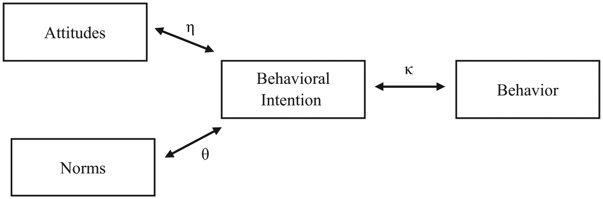
The TRA

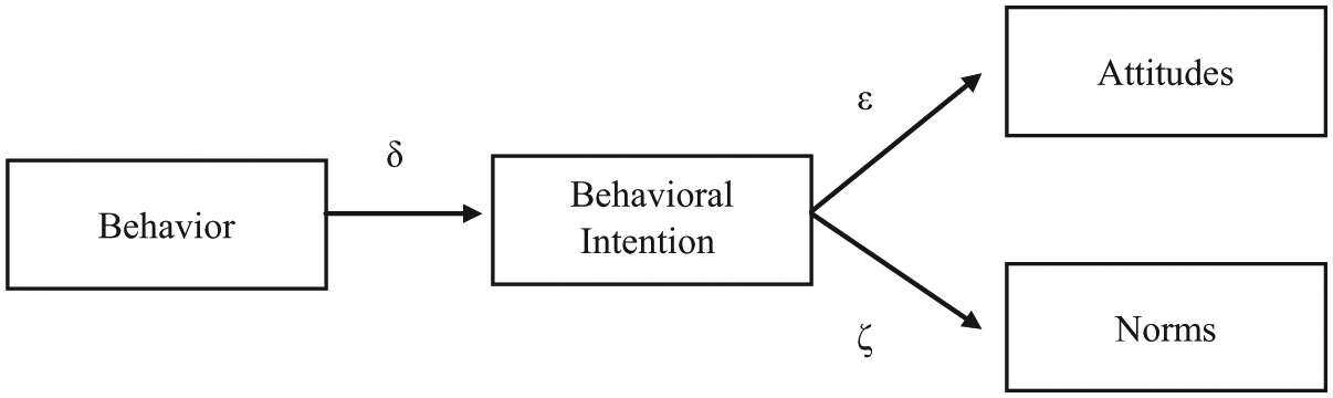
As Figure 1 illustrates, the TRA can be viewed as a cross-sectional causal model positing that volitional behavior (B) is a function of behavioral intention (I), with I conceived as the subjective probability that an action will be performed (Fishbein & Ajzen, 1975). As the sole determinant of B in the model, I is hypothesized to mediate completely the influence of attitude toward the behavior (A) and subjective norm (N) on B. As Figure 1 indicates, A and N are the only predictors of I, with A typically exhibiting stronger influence on I than does N (Armitage & Connor, 2001; O’Keefe, 2002). Conceptually, A “represents a person’s general favorableness or unfavorableness toward some stimulus object” (Fishbein & Ajzen, 1975, p. 216), the stimulus object being a specific B. In contrast, N is defined as “the person’s perception that most people who are important to him think that he should or should not perform the behavior in question” (Fishbein & Ajzen, 1975, p. 302). 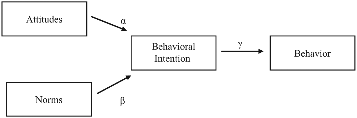Fishbein and Ajzen’s (1975) equation specifies the TRA’s main tenets, $B \sim I = (A) W_{1} + (N) W_{2}$ , with $W_{1}$ and $W_{2}$ being empirically determined weights. The regression of B onto I is presumed to be linear, and the regression of I onto A and N is presumed to be both linear and additive.

Figure 1.

The Theory of Reasoned Action.

The model presented in Figure 1 allows a spurious association between A and N, and generally, these constructs covary positively. Presumably, this positive covariation arises from causal forces antecedent to the model. For example, the existence of a common cause(s) that correlates either positively with both variables or negatively with both variables can produce such positive covariation.

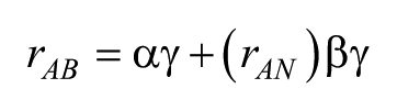
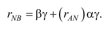
For this model to fit a set of data, two general conditions must be met. First, the three direct effect parameters in Figure 1, α, β, and γ, must be ample because for one variable to be considered a direct cause of another requires substantial covariation between them, or, in the case of α and β, substantial covariation after controlling for the effect of another posited cause. Second, the obtained values of the correlations unconstrained by estimation must not deviate substantially from their predicted values. Both the correlations between A and B and between N and B are unconstrained by estimation. Causal analysis indicates that the structure of this model predicts that

r_{A B} = α γ + (r_{A N}) β γ

and

r_{N B} = β γ + (r_{A N}) α γ .

Furthermore, when ordinary least squares (OLS) is employed to estimate the model’s parameters, the standardized estimates are,

α = \frac{(r_{A I} - r_{N I} r_{A N})}{(1 - r_{A N}^{2})},

β = \frac{(r_{N I} - r_{A I} r_{A N})}{(1 - r_{A N}^{2})},

and

γ = r_{I B} .

Substituting these parameter values into the preceding expressions for r_AB and r_NB yields the more elegant expressions,

r_{A B} = r_{A I} r_{I B}

and

r_{N B} = r_{N I} r_{I B},

for the predicted correlations, r_AB and r_NB.

The DTRA

The theoretical mechanisms by which the components of the TRA change, however, have not been elucidated. This lacuna is critical for theory, because the causal links in cross-sectional models arise from change processes.² A DTRA can be developed by considering the manner in which each of the four variables in the TRA change.³ Cases in which there is an absence of an exogenous shock were examined. Because both A and N are posited to be exogenous, in the absence of any force designed to change them, such as a persuasive message, no reason to expect them to change exists. Thus, for this model,

Δ N = 0

and

Δ A = 0

By the definition of the change operator, it follows that

N_{t} = N_{t - 1} = N_{0}

and

A_{t} = A_{t - 1} = A_{0} .

Hence, this model asserts that in the absence of a shock, such as an effective persuasive message, both A and N exhibit perfect first-order autoregression.

I, however, is endogenous in the TRA, its direct causes being both A and N. All three of these variables can be scaled on a continuum that ranges from extremely positive to extremely negative, so that it is sensible to speak of persons comparing them. This DTRA model posits that I changes when persons compare I with A and N, and adjusts I to reduce discrepancies. Converting this verbal proposition to a difference equation yields,

Δ I = Φ (N - I) + Ψ (A - I),

where 0 < Φ ≤ 1 and 0 < Ψ ≤ 1.

This equation implies that when A is more positive than I, then I will change in the direction of becoming more positive; whereas when A is more negative than I, then I will change in the direction of becoming more negative. Furthermore, when N is more positive than I, then change in I will be positive; whereas when N is more negative than I, then change in I will be negative.

The symbols Φ and Ψ represent the relative impact of A and N on I. The restriction on the values that the parameters Φ and Ψ may take indicate important features of how these variables affect I. Such restrictions are that I changes in the direction of A (N), so that no boomerang occurs (i.e., 0 < Φ and 0 < Ψ), and that this change does not become more extreme than A (N), so that no overshoot occurs (i.e., Φ ≤ 1 and Ψ ≤ 1).

Given a two-wave panel study, Equation 1 can be written in recursive form as,

I_{t + 1} = Φ N_{t} + Ψ A_{t} + Ω I_{t},

where Ω = 1 − Φ − Ψ,

and in which the subscripts refer to time, zero representing the initial measurement and one representing the subsequent measurement. The recursive equation has the intuitively appealing feature of predicting that I, at any given time, is determined completely by the immediately preceding (temporally) linear combination of A, N, and the previous I. As with A and N, I exhibits first-order autoregression. Because the model posits multiple causes of I, however, I does not exhibit perfect positive first-order autocorrelation.

The TRA also asserts that B is endogenous, I being its sole antecedent. This DTRA model claims that B is changed when persons compare their B with their I and adjust B proportionally to reduce any discrepancy between the two. Converting this verbal proposition to a difference equation yields,

Δ B = Λ (I - B),

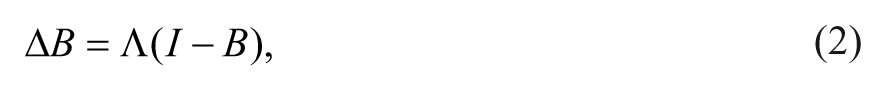
where 0 < Λ ≤ 1.

Equation 2 implies that when I is more positive than B, then change in B will be positive; whereas when I is more negative than B, then change in B will be negative. The proportionality constant, Λ, measures the proportion of the I − B discrepancy that is reduced. Again, the restrictions on the values that the parameter can assume reflect the theoretical proposition that boomerang and overshoot do not occur.

Writing Equation 2 in recursive form yields,

B_{t + 1} = Λ I_{t} + Π B_{t},

where Π = 1 − Λ.

This recursive form has the feature of predicting that B, at any given time, is determined completely by the immediately preceding (temporally) linear combination of I and B. B exhibits positive first-order autoregression, but because the model posits multiple causes, B is not expected to exhibit perfect positive first-order autocorrelation. Notably, to the extent that Ouellette and Wood’s (1998) claim that habit needs to be included in causal models of B is accurate, this effect is incorporated in this dynamic version of the TRA by the parameter Π. Consistent with this position, Webb and Sheeran’s (2006) meta-analysis of intention and behavior found that I has a smaller effect on B when habits are likely to be strong.

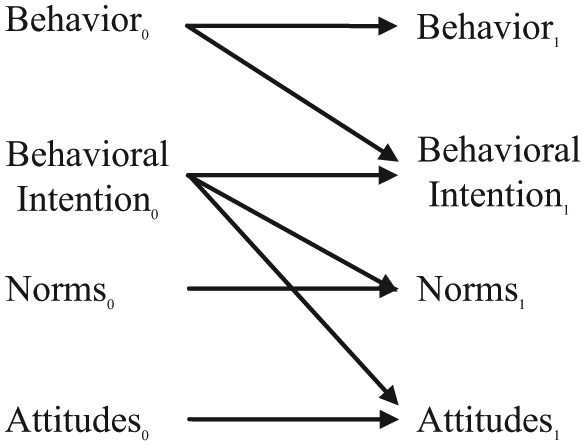
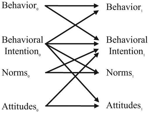
The recursive forms of these equations can be generalized and combined to produce the longitudinal causal model presented in Figure 2. The change equations provide the theoretical basis of this model, and Figure 2 follows logically from them. Measurements of A, N, I, and B taken at multiple times can be used to test this model, and by extension, the theory summarized in the change equations.

Figure 2.

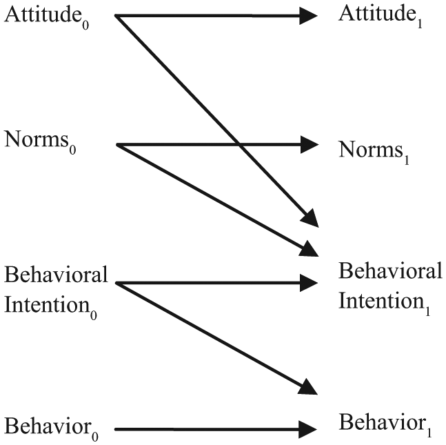
The longitudinal causal model produced by the Dynamic Theory of Reasoned Action.

Because in the absence of a shock, such as a persuasive message, there is no reason to expect A or N to change, these variables are in equilibrium. The equilibrium prediction for I can be obtained by setting the change equation for I equal to zero and solving. This procedure yields the following solution for I:

I = (\frac{Φ}{(Φ + Ψ)}) N + (\frac{Ψ}{(Φ + Ψ)}) A .

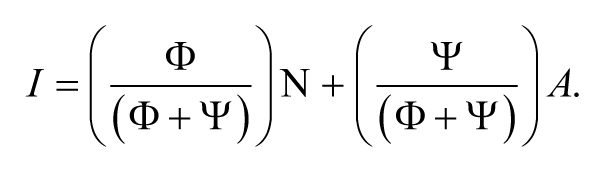
Therefore, the model has the intuitive appealing property that at equilibrium, I becomes a weighted sum of one’s A and N, such that the stronger the impact of the A − I discrepancy (i.e., Ψ) relative to the impact of the N − I discrepancy (i.e., Φ), the more heavily weighted is A in determining I. Conversely, the stronger the impact of the N − I discrepancy (i.e., Φ) relative to the impact of the A − I discrepancy (i.e., Ψ), the more heavily weighted is N in determining I.

The equilibrium prediction for B can be obtained by setting the change equation for B to zero and solving. This procedure yields the solution, B = I. Hence, at equilibrium, B becomes completely consistent, and hence correlated perfectly, with I.

A simulation was conducted to examine the implications of the DTRA for cross-sectional tests of the TRA. In addition to examining the fit of the cross-sectional TRA at each time point, the time necessary to reach equilibrium was examined.

Given the focus of this article on the fit of the cross-sectional TRA, it is valuable to scrutinize time to reach equilibrium as it is expected that, in the absence of an external shock, as the DTRA approaches equilibrium, the fit of the cross-sectional TRA will improve (Kaplan, Harik, & Hotchkiss, 2001). In addition, when the DTRA reaches equilibrium, it is expected that, in the absence of an external shock, it will stay in equilibrium; that is, it will be a stable equilibrium. At that point, the cross-sectional TRA is expected to exhibit perfect fit. Thus, the sooner the DTRA reaches equilibrium, the sooner will the cross-sectional TRA model begin to fit the data perfectly.

The time to reach equilibrium is expected to be a function of the strength of autoregression such that the stronger the autoregression parameters (i.e., Ω and Π) relative to the cross-lag parameters (i.e., Φ, Ψ, and Λ), the less time required to reach equilibrium. As the change equations for A and N indicate, in the absence of change, autoregression is perfect. Although strong, and even perfect, autoregression can result when a variable is changing, less than perfect autoregression implies that change must be occurring. In addition, generally, the lower the autoregression coefficients, the more change would be occurring. Ceteris paribus, the more change, the longer will a system take to reach equilibrium. Consequently, it is expected that varying the autoregression coefficients will vary the time taken for the system to reach equilibrium, which will, in turn, determine the time taken for the cross-sectional TRA to fit perfectly.

To examine this notion, Ω and Π were varied. The details of a simulation designed to test these propositions are presented subsequently.

Forward Simulation

Method

Seed distribution

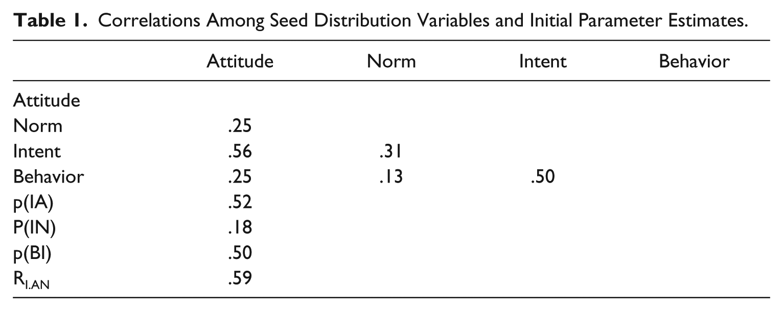
Initial distributions of each of the four key components of the TRA (A, N, I, and B) were constructed. Several criteria were employed when developing these distributions. First, a large sample, but not unreasonably large by social science standards, was deemed desirable. Second, the range of each variable was to be bounded in a manner found commonly in social science research. Third, uniformity in central tendency and dispersion for each variable was sought to simplify both cross-sectional and longitudinal comparisons. Fourth, a familiar and uniform (across variables) distribution shape was judged useful for comparison purposes. Pursuant to these goals, the distribution of each variable was composed of 1,600 hypothetical cases, scores ranged from 1 to 5 for each variable with a mean of 3.0, a standard deviation of 1.0, and the distribution was approximately normal with no skewness, but slight platykurtosis (−.498, s_e = .122).

These initial distributions were also created, so that the regression of B on I was linear, the regression of I on both A and N was linear, and the correlations among these four variables fit the cross-sectional TRA within sampling error. The initial correlation matrix is presented in Table 1, and testing the fit of the cross-sectional causal model with Hamilton and Hunter’s (1995) algorithm produced ample and reasonable parameter estimates for all postulated causal paths (see Table 2) and excellent fit, χ²(2, N = 1,600) = 1.37, p = .50, RMSE = .03.

Table 1.

Correlations Among Seed Distribution Variables and Initial Parameter Estimates.

	Attitude	Norm	Intent
Attitude
Norm	.25
Intent	.56	.31
Behavior	.25	.13	.50
p(IA)	.52
P(IN)	.18
p(BI)	.50
R_I.AN	.59

Table 2.

Summary of the Parameters.

DTRA	Weak	Moderate	Strong
Φ	.20	.15	.10
Ψ	.35	.25	.15
Ω	.45	.60	.75
Λ	.40	.25	.10
Π	.60	.75	.90
DRTRA	Weak	Moderate	Strong
λ	.60	.75	.90
Γ	.40	.25	.10
ζ	.60	.75	.90
Ξ	.40	.25	.10
Θ	.60	.75	.90
π	.40	.25	.10
DNTRA	Weak	Moderate	Strong
α	.40	.25	.10
δ	.60	.75	.90
β	.40	.25	.10
ϵ	.60	.75	.90
τ	.18	.14	.08
µ	.18	.14	.08
ϕ	.18	.14	.08
κ	.46	.58	.76
γ	.40	.25	.10
ρ	.60	.75	.90

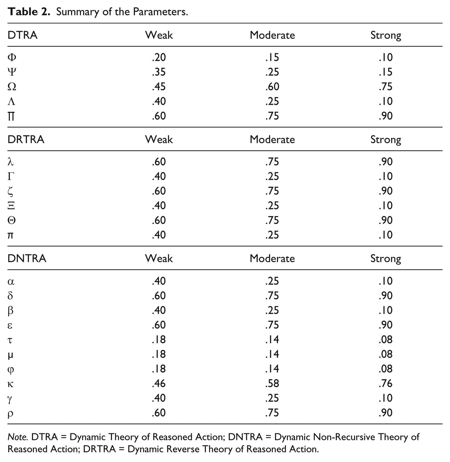
Note. DTRA = Dynamic Theory of Reasoned Action; DNTRA = Dynamic Non-Recursive Theory of Reasoned Action; DRTRA = Dynamic Reverse Theory of Reasoned Action.

Design

To simulate the change in the components of the TRA, it was necessary to specify reasonable values for the parameters. To assess the impact of differences in the parameters on the fit of the cross-sectional TRA, the autoregression parameters were varied and the cross-lag parameters were adjusted to meet the constraints specified in the change equations and their recursive forms. Table 2 presents the parameter values for the weak, moderate, and strong autoregression conditions.

Notably, in each condition, the autoregression parameters are larger than the cross-lag parameters, so that cognitive and behavioral inertia are deemed stronger causal forces than the impact of exogenous variables or the mediating variable. Moreover, in each condition, the A component is set so that it is stronger than the N component so as to comport with the empirical evidence (Armitage & Connor, 2001; O’Keefe, 2002).

Procedure

The recursive equations were employed to generate values for each of the four variables in the system over time. The iterative process was terminated when variable specific criteria for equilibrium or stability were reached.

Instrumentation

The number of iterations (trials) required for the system to reach equilibrium was assessed by examining the mean and the variance in the change in I and B. The impact of the change processes on the fit of cross-sectional tests of the TRA was assessed by examining three features of these models. First, the effect on the size and stability of the parameters was estimated. Second, the effect on model fit was examined. Third, the effect on the distributional properties of the variables that compose the model was assessed.

Results

A criterion of both the mean and the standard deviation in the change in I equaling zero to two decimal places (i.e., M_ΔI = S_ΔI < .005) for five consecutive trials was used to define equilibrium in I. From Table 3, it may be observed that the number of trials to reach this criterion increased as autoregression increased. The same criterion was employed to define the equilibrium in B (i.e., both M_ΔB < .005 and S_ΔB < .005 must be reached). Again, the number of trials to reach equilibrium increased as autoregression increased (see Table 3).⁴

Table 3.

Trials to Reach Equilibrium as a Function of Strength of Autoregression.

DTRA	Weak	Moderate	Strong	M
S(ΔI)	7	10	15	10.67
S(ΔB)	12	18	34	21.33
M	9.5	14	24.5
DRTRA	Weak	Moderate	Strong	M
S(ΔA)	14	22	45	27
S(ΔN)	14	22	45	27
S(ΔI)	10	15	30	18.34
M	12.67	19.667	40
DNTRA	Weak	Moderate	Strong	M
S(ΔA)	10	14	27	17
S(ΔN)	10	14	28	17.33
S(ΔI)	3	5	10	6
S(ΔB)	10	14	27	17
M	8.25	11.75	23

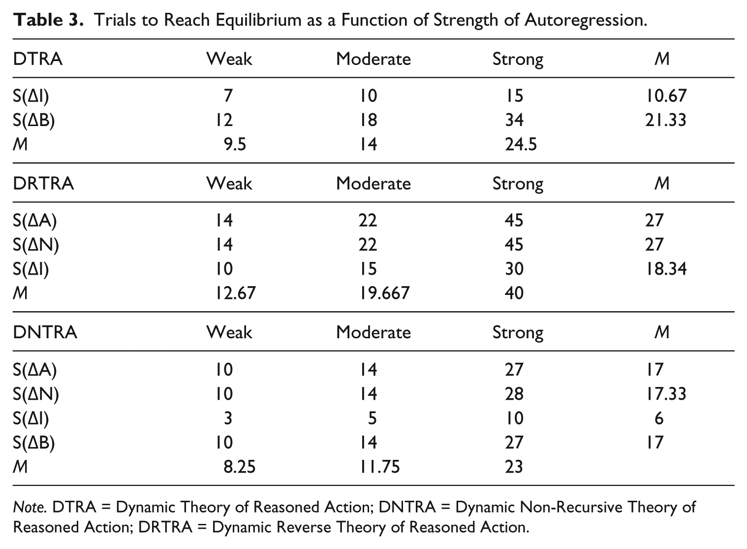
Note. DTRA = Dynamic Theory of Reasoned Action; DNTRA = Dynamic Non-Recursive Theory of Reasoned Action; DRTRA = Dynamic Reverse Theory of Reasoned Action.

From these observations, several conclusions may be drawn. First, as a result of being at the end of the causal process, B took longer to reach equilibrium (across autoregression conditions, M = 21.33 trials) than the mediator I (across autoregression conditions, M = 10.67 trials). The difference was more pronounced when autoregression was strong (a difference of 19 trials) than when it was moderate (a difference of 8 trials) than when it was weak (a difference of 5 trials). Second, the effect of the magnitude of autoregression on trials to criterion was more pronounced for B than for I. Specifically, the difference in trials to criterion between the moderate and weak autoregression conditions was 3 trials for I, but 6 trials for B. The difference between the strong and moderate autoregression conditions was 5 trials for I, but 16 trials for B.

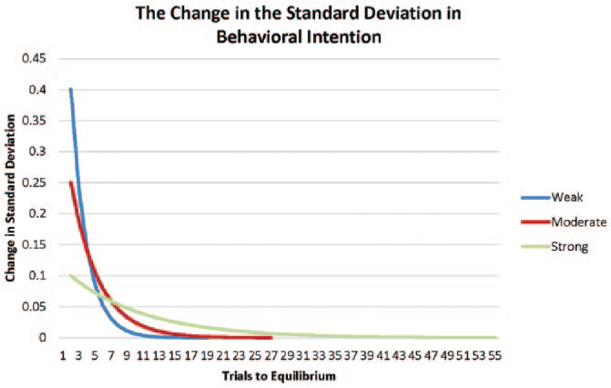
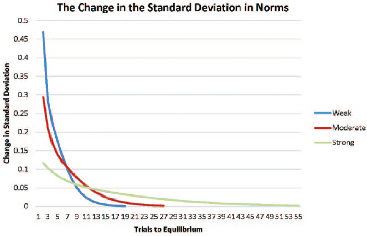
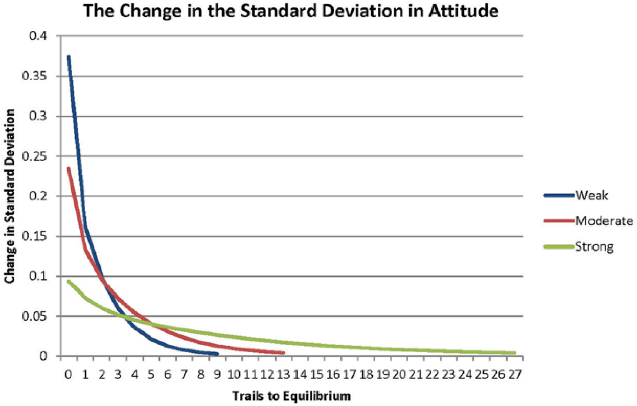
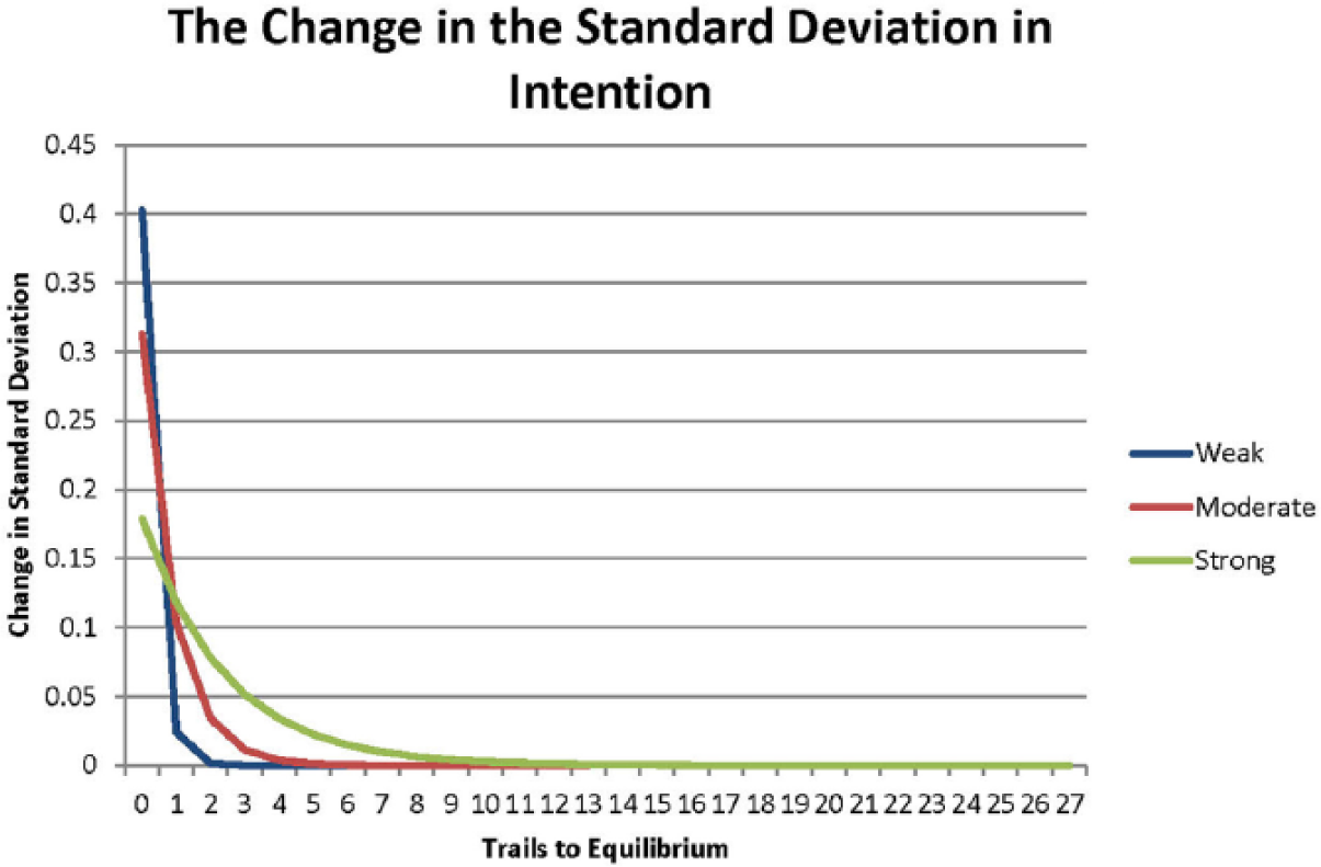
Third, the rapidity of the descent to equilibrium varied as a function of the strength of autoregression. Figure 3 presents the standard deviation, calculated to five decimal places, in the change in I as a function of trials (time). In all conditions, the standard deviation in the change in I decreased exponentially as a function of time. Notably, although the DTRA with the low autoregression parameters reach equilibrium faster than the DTRA with high autoregression parameters, the latter never deviated substantially from equilibrium. In fact, their deviations from equilibrium are smaller for most trials than are the deviations produced by the DTRA with moderate or small autoregression parameters.

Figure 3.

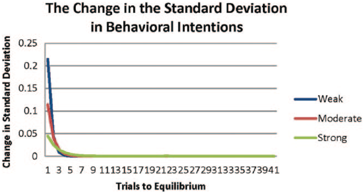
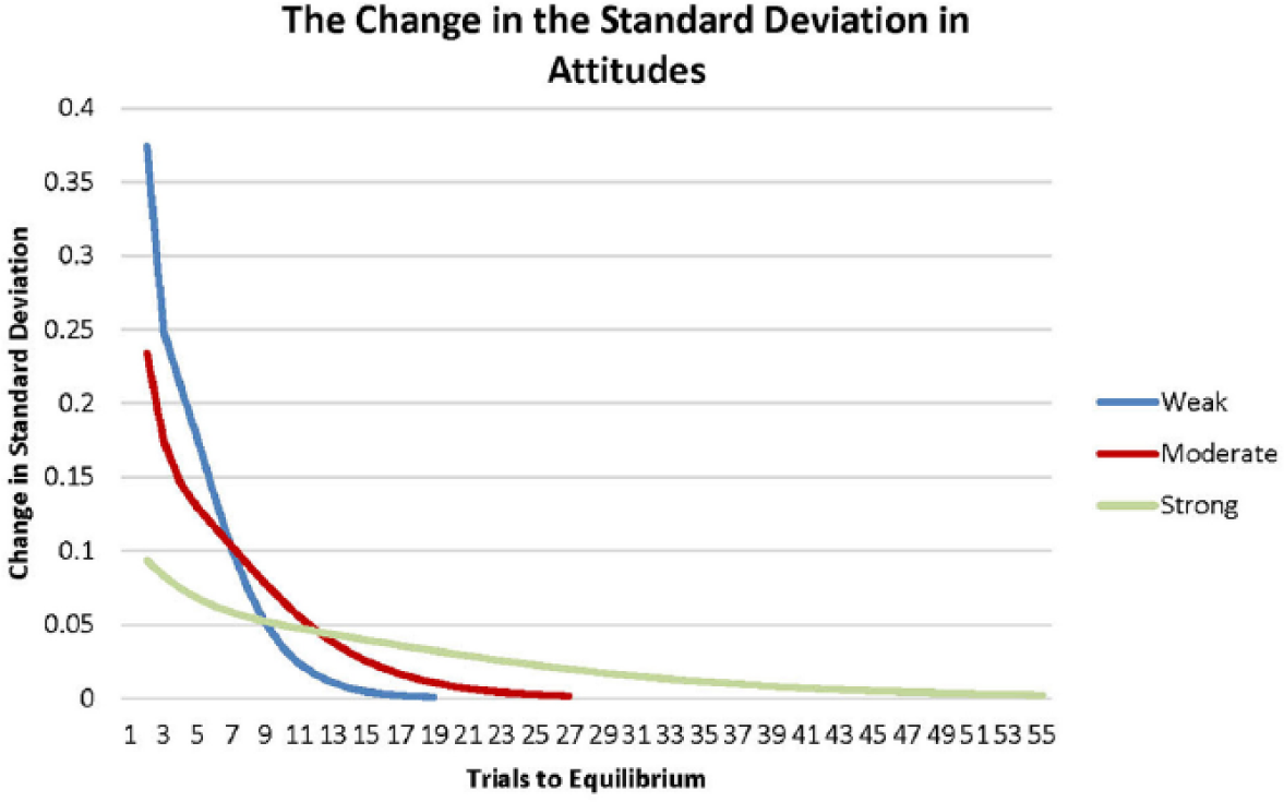
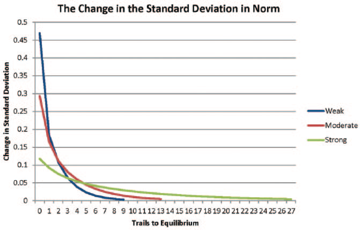
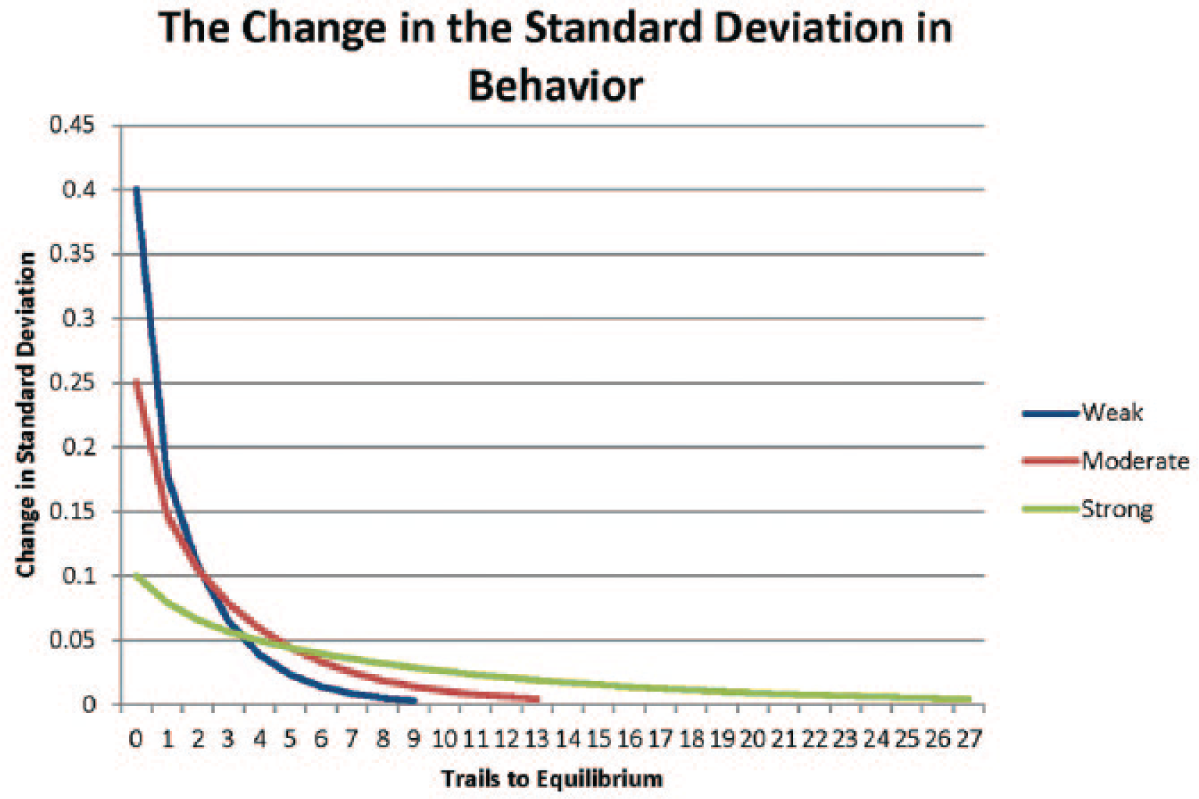
The descent of the standard deviation in the change in I as a function of the time and the strength of autoregression for the DTRA.

Figure 4 presents the standard deviation, calculated to five decimal places, in the change in B as a function of time. As with I, in all conditions, the standard deviation in the change in B decreased exponentially as a function of time. In addition, as with I, although the DTRA with low autoregression parameters reached equilibrium faster than the DTRA with high autoregression parameters, the latter never deviated substantially from equilibrium, and their deviations from equilibrium are smaller for most trials than are the deviations produced by the DTRA with moderate or small autoregression parameters.

Figure 4.

The descent of the standard deviation in the change in B as a function of the time and the strength of autoregression for the DTRA.

The features of the cross-sectional model that was examined included various descriptive statistics (e.g., the variance in I and the variance in B⁵), parameter estimates (the path coefficients and the multiple correlation of I with A and N), and measures of model fit (chi-square and the root mean squared error). Each will be considered in turn.

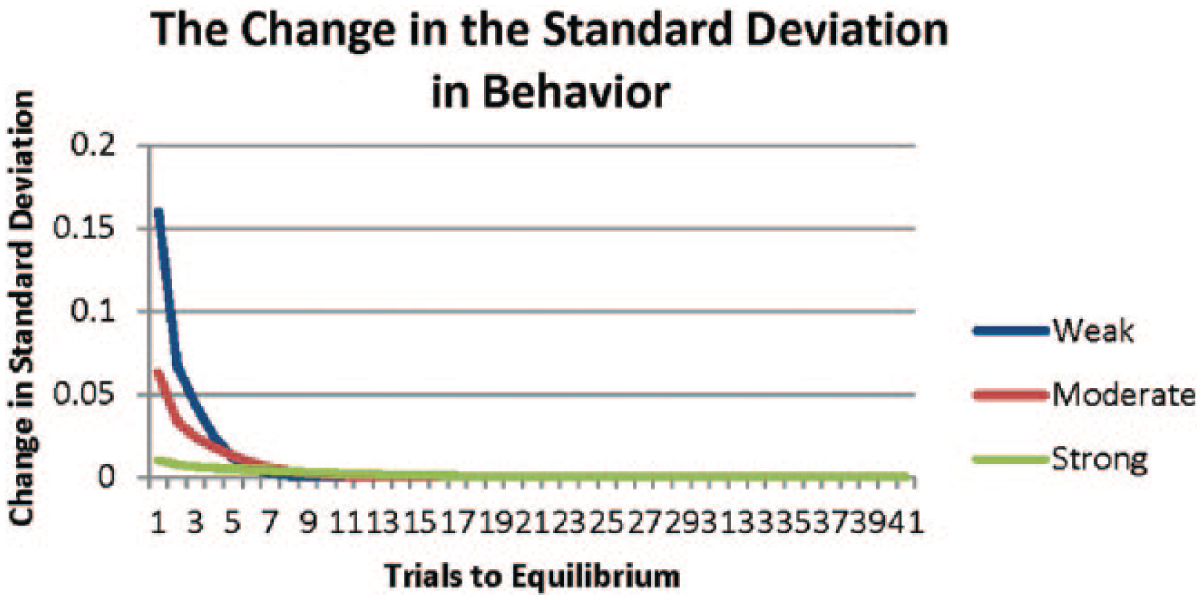
As Table 4 indicates, the values of the variances in I and B at equilibrium varied little as a function of the strength of autoregression, stabilizing in the mid .6 range. The number of trials required to reach these stable values did, however, vary substantially for the two variables and as a function of the strength of autoregression. Moreover, these relationships parallel those found for the variance in the change in I and the variance in the change in B. Specifically, the variance in I stabilized more rapidly (across autoregression conditions, M = 9.67 trials) than the variance in B (across autoregression conditions, M = 24.33 trials), trials to stabilize increased more than proportionally as the strength of autoregression increased (M = 8.0, 15.0, and 28.0 for weak, moderate, and strong autoregression, respectively), and the difference in trials to stabilize increased more rapidly for B than for I.

Table 4.

Values of the Variance in the Endogenous Variables at Equilibrium (Trials to Stabilize) as a Function of Strength of Autoregression.

DTRA	Weak	Moderate	Strong	M
V(I)	.65 (5)	.65 (9)	.64 (15)	9.67
V(B)	.65 (11)	.65 (21)	.63 (41)	24.33
M	8	15	28
DRTRA	Weak	Moderate	Strong	M
V(A)	1 (15)	1 (26)	.99 (59)	33.33
V(N)	1 (15)	1 (26)	.99 (59)	33.33
V(I)	1 (10)	1 (18)	1 (50)	26
M	13.33	23.33	56
DNTRA	Weak	Moderate	Strong	M
V(A)	.56 (12)	.54 (12)	.52 (23)	0.54
V(N)	.56 (3)	.54 (5)	.51 (15)	0.54
V(I)	.56 (2)	.54 (4)	.52 (12)	0.54
V(B)	.56 (9)	.54 (9)	.51 (28)	0.54
M	0.56	0.54	0.52

Note. DTRA = Dynamic Theory of Reasoned Action; DNTRA = Dynamic Non-Recursive Theory of Reasoned Action; DRTRA = Dynamic Reverse Theory of Reasoned Action.

Data pertinent to the four cross-sectional parameters obtained after the system reached equilibrium are presented in Table 5. These parameters were estimated in this and all subsequent simulations using the ordinary least squares criterion. Specifically, p(IA) is obtained by regressing I on A, controlling for N; P(IN) is obtained by regression I on N, controlling for A; and p(BI) is obtained by regressing B on I. From this table, one may observe that the path linking A and I (p_IA) stabilized in the middle to upper .7 range, the path linking N and I (p_IN) being substantially lower stabilized in the mid .4 to .5 range, the path linking I and B (p_BI) stabilized at 1.00, and the multiple correlation of I with A and N (R_I.AN) stabilized at 1.00. Notably, the latter two parameters indicate that the endogenous variables are predicted without error to two decimal points when the model reaches an equilibrium state. Also notable is that the point at which the p_IA estimate stabilized decreased slightly with increasing autoregression, whereas the point at which the p_IN estimate stabilized increased slightly with increasing autoregression. For each of the parameter estimates, the number of trials taken to reach stability increased with increasing autoregression, albeit not proportionally, the trend for the p_BI estimate being particularly pronounced.

Table 5.

Values of Parameter Estimates at Equilibrium (Trials to Stabilize) as a Function of Strength of Autoregression.

DTRA	Weak	Moderate	Strong
p(IA)	.79 (3)	.78 (4)	.75 (11)
p(IN)	.45 (5)	.47 (12)	.50 (12)
p(BI)	1.00 (7)	1.00 (11)	1.00 (27)
R_I.AN	1.00 (3)	1.00 (5)	1.00 (9)
DRTRA	Weak	Moderate	Strong
p(IB)	1.00 (5)	1.00 (8)	1.00 (21)
p(AI)	1.00 (8)	1.00 (13)	1.00 (33)
p(NI)	1.00 (8)	1.00 (13)	1.00 (33)
DNTRA	Weak	Moderate	Strong
p(IA)	.50 (5)	.50 (5)	.50 (5)
p(IN)	.50 (5)	.50 (5)	.50 (5)
p(BI)	1.00 (5)	1.00 (11)	1.00 (29)
p(IB)	1.00 (5)	1.00 (10)	1.00 (29)
p(AI)	1.00 (5)	1.00 (10)	1.00 (29)
p(NI)	1.00 (5)	1.00 (10)	1.00 (29)

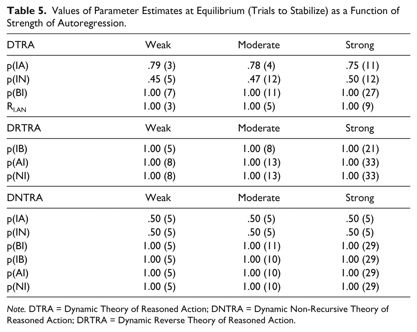
Note. DTRA = Dynamic Theory of Reasoned Action; DNTRA = Dynamic Non-Recursive Theory of Reasoned Action; DRTRA = Dynamic Reverse Theory of Reasoned Action.

The root mean squared error (RMSE) was employed as a measure of the fit of the cross-sectional model. Perfect fit was defined as occurring when the RMSE reduced to zero rounded to two decimal places. The number of trials to reach zero increased with increasing autoregression with 10 trials being required when autoregression was weak, 13 trials when autoregression was moderate, and 30 trials when autoregression was strong.⁶

Discussion

Strong autoregression in I and B suggests strong cognitive inertia, in the case of I, and powerful habit strength, or behavioral inertia, in the case of B. Although in the strong autoregression condition, the model began closer to equilibrium and approximated it closely over trials, contrary to expectations increasing autoregression resulted in the four variable system reaching equilibrium less rapidly. The strong I autoregression parameter implied a weaker effect of A and N on I, and the strong B autoregression parameter implied a weaker effect of I on B. Combined, these forces slowed the rate of change in the endogenous variables that was necessary to reach equilibrium.

A second implication of the model is that convergence is more rapid for proximal variables in the causal sequence. Put differently, in this simulation, I reached equilibrium more rapidly than did B, this effect being more pronounced with increasing autoregression.

To anticipate one objection, a question may be raised as to why model the TRA longitudinally rather than the TPB with its more extensive variable set. One reason is that it is useful to begin to understand the simpler model before proceeding to the more complex model. Another answer, however, is that perhaps the list of variables in the TPB may be reducible. Habit (Ouellette & Wood, 1998), for example, may be reduced to the autoregression parameter linking B with itself at a previous point in time. Efficacy, or perceived behavioral control, may be modeled by reversing the TRA (i.e., perhaps when B is less under one’s control, B drives I which, in turn, drives both A and N). Although much social scientific theory is often linked with variable proliferation, in some other disciplines, an important function of theory is variable reduction as well. Perhaps some variables are created by some social scientists as a substitute for longitudinal parameters or differing longitudinal models. This possibility is explored in a second simulation.

Reverse Simulation

The cross-sectional reversed model (RTRA) is presented in Figure 5. This model includes three correlations (or covariances) that are unconstrained by estimation, the A-B, N-B, and A-N correlations. Although it appears not to be well known, and although it is counterintuitive, both the TRA and RTRA make exactly the same predictions as to the value of the A-B and N-B correlations (see the appendix). In addition, the RTRA predicts that the A-N correlation is the product of the A-I and N-I correlations, that is, r_AN = (r_AI) × (r_NI).

Figure 5.

The Reverse Theory of Reasoned Action.

The conceptual value of the RTRA may be as an explanatory mechanism of involuntary behavior. Specifically, if persons were to believe that an action was not controllable for them (i.e., low perceived behavioral control), then it is reasonable to posit that their subjective probability estimate of what they will do (i.e., their intention) is driven by present action. That is, if particular action is deemed uncontrollable, then one is likely to conclude that one will engage in it (or fail to). Such fatalism would result in such persons noting that they intend to continue their present course of action, as they would have no ability to do otherwise. These intentions would, in term, shape subsequent attitudes that are formed about the behavior and perceptions of the normative beliefs of significant others (or indeed, it may shape those judged to be significant others) toward the behavior.

This process may also explain the substantial amount of behavioral inertia observed in particular domains of action. For example, if one were to think of smoking as behavior over which volitional control is low, then it may be more useful to predict future behavior from current behavior, thus employing the RTRA for explanatory and predictive power. Given that many smokers are addicted to nicotine, current smoking behavior would be predictable from prior smoking. In addition, behavioral intentions would be predictable from knowing prior behavior. It is instructive on this point to note that Fishbein and Ajzen (2010) grant that some research demonstrates that prior behavior has an effect on behavioral intentions and that their theory fails to explain this link. Finally, consistent with cognitive dissonance theory and self-perception theory, these intentions would shape subsequent attitudes that are formed about smoking and perceptions of what significant others think about smoking, or possibly the others with whom one associates.

A longitudinal version of this model, the DRTRA, is presented in Figure 6. Given that B is exogenous in the model, in the absences of a shock (e.g., a persuasive message) designed to change it, no change is expected to exist. Thus,

Δ B = 0

and

B_{t} = B_{t - 1} = B_{0} .

Hence, this model asserts that in the absence of a shock, B exhibits perfect first-order autoregression.

Figure 6.

The longitudinal causal model produced by the Dynamic Reverse Theory of Reasoned Action.

I, on the other hand, is endogenous in the RTRA, its direct cause being B, and this DRTRA model posits that I may change when persons compare I and B, adjusting I proportionally to reduce any discrepancies. It follows that

Δ I = Γ (B - I),

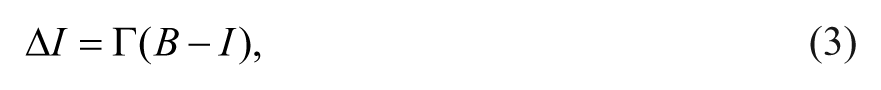
where 0 < Γ ≤ 1.

This equation implies that when B is greater than I, then I will increase; whereas when B is less than I, then I will decrease.

Γ represents the relative impact of B on I. The restriction on the values that Γ may take indicates that I changes in the direction of B, so that no boomerang or overshoot occur. Writing the equation in recursive form yields,

I_{t + 1} = Γ B_{t} + K I_{t},

where K = 1 − Γ.

This equation predicts that I at any given time is determined completely by the immediately preceding (temporally) linear combination of B and I. Similar to B, it posits that I exhibits first-order autoregression. Because the model posits that I is caused by B as well, I is not, however, expected to exhibit perfect positive first-order autocorrelation.

The RTRA also asserts that both A and N are endogenous, I being the sole antecedent of each. This DRTRA model claims that A is changed when persons compare A and I, adjusting A proportionally to reduce discrepancies. This same comparison process occurs for N as well; persons compare N with I adjusting N proportionally to reduce discrepancies. Formally,

Δ A = H (I - A),

where 0 < H ≤ 1,

and

Δ N = Θ (I - N),

where 0 < Θ ≤ 1.

Equation 4 implies that when I is greater than A, then A will increase; whereas when I is less than A, then A will decrease. The proportionality constant, ζ, measures the proportion of the I-A discrepancy that is reduced. Equation 5 implies that when I is greater than N, then change in N is positive; whereas when I is less than N, then change in N is negative. The parameter, Θ, measures the proportion of the I-N discrepancy that is reduced. Again, the restrictions on the values that the parameters can assume reflect the theoretical proposition that boomerang and overshoot do not occur.

Writing these equations in recursive form yields,

A_{t + 1} = H I_{t} + Ξ A_{t},

where Ξ = 1 − H,

and

N_{t + 1} = Θ I_{t} + M N_{t},

where M = 1 − Θ.

The former has the feature of predicting that A, at any given time, is determined completely by the immediately preceding (temporally) linear combination of I and A. A exhibits positive first-order autoregression, but because the model posits multiple causes, it is not expected to exhibit perfect positive first-order autocorrelation. The same point applies to the latter; predicting N at any given time is determined completely by the immediately preceding (temporally) linear combination of I and N. Similar to A, N exhibits positive first-order autoregression, but because the model posits multiple causes, N is not expected to exhibit perfect positive first-order autocorrelation.

The recursive equations can be generalized and combined to produce the longitudinal causal model presented in Figure 6. The change equations provide the theoretical basis of this model; thus, Figure 6 follows logically from them. Measurements of A, N, I, and B taken at multiple times can be used to test this model, and by extension, the theory summarized in the change equations.

Because in the absence of a shock, such as a persuasive message, no reason to expect B to change exists; therefore, B is in equilibrium. The equilibrium prediction for I can be obtained by setting the change equation for I to zero and solving. This procedure yields the solution, B = I. Therefore, the model has the property that at equilibrium, I and B become completely consistent. In addition, setting Equations 4 and 5 to zero and solving yields the solutions, I = A and I = N. Therefore, at equilibrium, A and N become completely consistent with I.

A second simulation was conducted to examine the implications of the DRTRA for the fit of cross-sectional tests of the RTRA. In addition to examining the fit of the cross-sectional RTRA at each time point, the time necessary to reach equilibrium was examined. As in the first simulation, the time taken to reach equilibrium was expected to decrease as the strength of the autoregression parameters increase relative to the strength of the cross-lag. To examine this notion, the autoregression parameters were varied.

Method

Seed distribution

The same initial distributions of each of the four key components of the DTRA simulation (A, N, I, and B) were used for the simulation of the DRTRA.

Design

Parameter values were assigned using the same procedures that were employed in the first simulation. These values are presented in Table 2.

Instrumentation

The same criteria employed in the first simulation for assessing equilibria were employed in this simulation as well. Similarly, the effect on the size and stability of the parameters, model fit, and the distributional properties of the variables that compose the model were assessed.

Results

Table 3 indicates that similar to the findings of the DTRA simulation, it took longer for distal endogenous variables, A and N, to reach equilibrium (M = 27 trials) than it did for the mediator, I (M = 18.34 trials). Also consistent with findings from the DTRA simulation, this difference was more pronounced when autoregression was strong (a difference of 15 trials) than when it was moderate (a difference of 7 trials) or weak (a difference of 4 trials).

Second, the effect of autoregression on trials to criterion was more pronounced for A and N than for I. Specifically, the difference between the moderate and weak autoregression conditions was 5 trials for I, but 8 trials for both A and N. The difference between the strong and moderate autoregression conditions was 15 trials for I, but 23 trials for A and N.

Third, the rapidity of the descent to equilibrium varied as a function of the strength of autoregression. Figure 7 presents the standard deviation, calculated to five decimal places, in the change in I as a function of time. In all conditions, the standard deviation in the change in I decreased exponentially as a function of time. In addition, although the DRTRA with low autoregression parameters reached equilibrium faster than the DRTRA with high autoregression parameters, the latter never deviate substantially from equilibrium, and their deviations from equilibrium are smaller for most trials than are the deviations produced by the DRTRA with moderate or small autoregression parameters.

Figure 7.

The descent of the standard deviation in the change in I as a function of the time and the strength of autoregression for the Dynamic Reverse Theory of Reasoned Action (DRTRA).

Figure 8 presents the standard deviation, calculated to five decimal places, in the change in A as a function of trials. In all conditions, the standard deviation in the change in A decreased exponentially as a function of time. Again, although the model with low autoregression parameters reached equilibrium faster than the model with high autoregression parameters, the latter differ modestly from equilibrium at most time points. Moreover, at many time points, they deviate less from equilibrium than do the moderate or small autoregression parameters.

Figure 8.

The descent of the standard deviation in the change in A as a function of the time and the strength of autoregression for the Dynamic Reverse Theory of Reasoned Action (DRTRA).

Figure 9 presents the standard deviation, calculated to five decimal places, in the change in N as a function of time. As with A, in all conditions, the standard deviation in the change in N decreased exponentially as a function of time. Once again, the model with low autoregression parameters reached equilibrium faster than the model with high autoregression parameters. Nevertheless, the latter differ modestly from equilibrium at most time points. In addition, at many time points, they deviate less from equilibrium than do the moderate or small autoregression parameters.

Figure 9.

The descent of the standard deviation in the change in N as a function of the time and the strength of autoregression for the Dynamic Reverse Theory of Reasoned Action (DRTRA).

The features of the cross-sectional model examined included various descriptive statistics, parameter estimates, and measures of model fit. Each will be considered in turn.

As Table 4 indicates the values of the variances in I, A, and N at equilibrium varied little as a function of the strength of autoregression, stabilizing at .99 or 1. The number of trials required to reach these stable values did, however, vary substantially for the three variables and as a function of the strength of autoregression. Specifically, the variance in I stabilized more rapidly (M = 26 trials) than the variance in A or N (M = 33.33 trials), trials to stabilize increased more than proportionally as the strength of autoregression increased (M = 13.33, 23.33, and 56 for weak, moderate, and strong autoregression, respectively), and the difference in trials to stabilize increased more rapidly for A and N than for I.

Data pertinent to the three parameters are presented in Table 5. The path linking B and I, p(IB) was obtained by regressing I on B, p(AI) by regressing A on I, and p(NI) by regressing N on I. From this table, one may observe that the path linking B and I (p_IB), A and I (p_AI), and N and I (p_NI) all stabilized at 1.00. Notably, all parameters indicate that the endogenous variables are predicted without error to two decimal points when the model reaches an equilibrium state. Also notable is that the number of trials taken to reach stability increased with increasing autoregression for all p_IB, p_AI, and p_NI estimates, albeit not proportionally. The same trend, taking longer for the distal endogenous variables to reach equilibrium, occurred. In the weak autoregression condition, the p_IB estimate stabilized after 5 trials, but it took both the p_AI and p_NI estimates 8 trials. This difference increased as autoregression increased. For the moderate autoregression condition, the number of trials to reach equilibrium for the p_IB estimate was 8 trials, but it took the p_AI and p_NI 13 trials. Finally, for the strong autoregression condition, the number of trials to reach equilibrium for the p_IB estimate was 21 trials, but it took p_AI and p_NI 33 trials.

Perfect fit of the cross-sectional model was again defined as occurring when the RMSE reduced to zero rounded to two decimal places. The number of trials to reach zero increased with increasing autoregression with 5 trials being required when autoregression was weak, 8 trials when autoregression was moderate, and 20 trials when autoregression was strong.

Discussion

Several of the patterns observed in the first simulation were observed in the simulation of the DRTRA. For example, the number of trials required for I, A, and N to stabilize increased more than proportionally with increasing autoregression. Moreover, more trials to stabilize were required for the distal endogenous variables, A and N, than for the more proximal endogenous variable, I. Comparatively, however, at all levels of autoregression more trials to stabilize were required for the one comparable parameter, I, in the DRTRA than the DTRA.

The DRTRA parameters stabilized at perfect prediction (i.e., r = 1.0) as would be expected when all endogenous variables posited to have a single cause (cf. r_IB in the forward simulation). Once again, trials to reach perfect fit increased more than proportionally as a function of increasing autoregression. Furthermore, across all levels of autoregression, more trials were required to reach perfect fit for the DRTRA than the DTRA.

If the DTRA modeled voluntary behavior effectively, and if the DRTRA modeled involuntary behavior effectively, the issue of how action that includes both voluntary and involuntary elements is to be modeled arises. One possibility is that a non-recursive version of the TRA could be transformed into a Dynamic Non-Recursive Theory of Reasoned Action (DNTRA). This possibility is explored in a third simulation.

Non-Recursive Simulation

The longitudinal extension appears in Figure 10 and Figure 11. Incorporating elements of both the DTRA and the DRTRA, no variable is exogenous. Instead, I is driven by both A and N as in the DTRA, B is driven by I as in the DTRA, I is driven by B as in the DRTRA, and both A and N are driven by I as in the DRTRA.

Figure 10.

The Non-Recursive Theory of Reasoned Action.

Figure 11.

The longitudinal causal model produced by the Dynamic Non-Recursive Theory of Reasoned Action.

The change in A is given by

Δ A = ζ (I - A),

so that at equilibrium A = I. In recursive form,

A_{t + 1} = ζ I_{t} + δ A_{t},

where δ = 1 − ζ.

Similarly, the change in N can be expressed as,

Δ N = ω (I - N),

so that at equilibrium N = I. In recursive form,

N_{t + 1} = ω I_{t} + ε N_{t},

where ϵ = 1 − ω.

The change in B is given by,

Δ B = ν (I - B),

and thus, at equilibrium B = I. In recursive form,

B_{t + 1} = ν I_{t} + ρ B_{t},

where ρ = 1 − ν.

Finally, the change in intentions can be expressed as,

Δ I = τ (A - I) + μ (N - I) + φ (B - I) .

At equilibrium, intentions become a weighted sum of the effect of A, N, and B. Specifically,

I = (\frac{τ A}{1 - κ}) + (\frac{μ N}{1 - κ}) + (\frac{φ B}{1 - κ}),

where κ = 1-τ - µ − ϕ.

In recursive form,

I_{t + 1} = τ A_{t} + μ N_{t} + φ B_{t} + κ I_{t} .

Method

Seed distribution

The same initial distributions of each of the four key components of the DTRA and DRTRA simulations (A, N, I, and B) were used for the simulation of the DNTRA.

Design

Parameter values were assigned using the same procedures that were employed in the first simulations. These values are presented in Table 2.

Instrumentation

The same criteria employed in the other simulations for assessing equilibria were employed in this simulation as well. Similarly, the effects on the size and stability of the parameters, model fit, and the distributional properties of the variables that compose the model were assessed.

Results

As Table 3 indicates, similar to the DTRA and DRTRA simulations, it took longer for the non-mediator variables, A, N, and B, to reach equilibrium (M_A = 17, M_N = 17.3, M_B = 17 trials) than it did for the mediator, I (M = 6 trials). Also consistent with the other simulations, this difference was more pronounced when autoregression was strong (a difference of 17 for trials for B and I and A and I, and 18 trials for N and I) than when it was moderate (a difference of 9 trials in each case) or weak (a difference of 7 trials in each case).

Second, the effect of autoregression on trials to criterion was more pronounced for A, N, and B than for I. Specifically, the difference between the moderate and weak autoregression conditions was 2 trials for I, but 4 trials for B, A, and N. Furthermore, the difference between the strong and moderate autoregression conditions was 5 trials for I, but 13 trials for B, 13 trials for A, and 14 trials for N.

Figure 12 presents the standard deviation, calculated to five decimal places, in the change in A as a function of trials. In all conditions, the standard deviation in the change in A decreased exponentially as a function of time. As with the other simulations, the descent for the low autoregression condition was steeper than the descent for the moderate autoregression condition than for the high autoregression condition. In addition, as with the other simulations, in the high autoregression condition, the departure from equilibrium was generally modest across trials.

Figure 12.

The descent of the standard deviation in the change in A as a function of the time and the strength of autoregression for the DNTRA.

Figure 13 presents the standard deviation, calculated to five decimal places, in the change in N as a function of time. As with A, in all conditions, the standard deviation in the change in N decreased exponentially as a function of time. The same pattern of steepness of descent and departure from equilibrium was observed for these curves as with A.

Figure 13.

The descent of the standard deviation in the change in N as a function of the time and the strength of autoregression for the DNTRA.

Third, the rapidity of the descent of I to equilibrium varied as a function of the strength of autoregression. Figure 14 presents the standard deviation, calculated to five decimal places, in the change in I as a function of trials (time). In all conditions, the standard deviation in the change in I decreased exponentially as a function of time, and the same pattern of steepness of descent to equilibrium and departure from equilibrium was observed in these figures as was observed for A and N.

Figure 14.

The descent of the standard deviation in the change in I as a function of the time and the strength of autoregression for the DNTRA.

Figure 15 presents the standard deviation, calculated to five decimal places, in the change in B as a function of time. As with I, in all conditions, the standard deviation in the change in B decreased exponentially as a function of time. The same pattern of steepness of descent to equilibrium and departure from equilibrium was observed in these figures as was observed for A, N, and I.

Figure 15.

The descent of the standard deviation in the change in B as a function of the time and the strength of autoregression for the DNTRA.

The features of the cross-sectional model examined included various descriptive statistics, parameter estimates, and measures of model fit. Each will be considered in turn.

As Table 4 indicates the values of the variances in A, N, I, and B at equilibrium varied little as a function of the strength of autoregression, stabilizing in the mid .50 range. The number of trials required to reach these stable values did, however, vary substantially for the four variables and as a function of the strength of autoregression. Specifically, the variance in I stabilized more rapidly (M = 6 trials) than the variance in A (M = 15.7 trials), N (M = 7.7 trials), and B (M = 15.3 trials), and trials to stabilize increased more than proportionally as the strength of autoregression increased (M = 6.5, 7.5, and 19.5 for weak, moderate, and strong autoregression, respectively).

Data pertinent to the six parameters are presented in Table 5. From the simulation data, the parameters were estimated for the TRA parameters, and then were estimated from the RTRA parameters. Thus, non-recursive estimates were not employed; rather, the parameters treat the two cross-sectional models separately. One may observe that p_IA and p_IN stabilized at .50; whereas p_BI, p_IB, p_AI, and p_NI all stabilized at 1.00. Notably, the endogenous variables are predicted without error to two decimal points when the model reaches equilibrium. Also notable is that the number of trials taken to reach stability increased with increasing autoregression for all estimates, albeit not proportionally. The same trend, taking longer for the non-mediator variables (A, N, and B) to reach equilibrium than the mediating variable (I), occurred. In the weak autoregression condition, the p_IB estimate stabilized after 5 trials, but it took both the p_AI and p_NI estimates 8 trials. This difference increased as autoregression increased. For the moderate autoregression condition, the number of trials to reach equilibrium for the p_IB estimate was 8 trials, but it took the p_AI and p_NI 13 trials. Finally, for the strong autoregression condition, 21 trials were required to reach equilibrium for the p_IB estimate, but it took the p_AI and p_NI estimates 33 trials.

Perfect fit was again defined as the RMSE reducing to zero, rounded to two decimal places. The number of trials to reach zero increased with increasing autoregression. For the DTRA cross-sectional model, 3 trials were required when autoregression was weak, 4 trials when autoregression was moderate, and 12 trials when autoregression was strong. The comparable figures for the DRTRA cross-sectional model were 3, 4, and 12.

Discussion

Several of the patterns observed in the first two simulations were observed in the simulation of the DNTRA. Once again the number of trials required for I, A, N, and B to stabilize increased more than proportionally with increasing autoregression. Moreover, fewer trials to stabilize were required for the mediating variable, I, than for A, N, and B, all of which took the same number of trials to reach equilibrium. Comparatively, at all levels of autoregression, fewer trials were required for I to stabilize for the DNTRA than the DTRA and the DRTRA. Moreover, at all levels of autoregression, fewer trials were required for B to stabilize for the DNTRA than the DTRA, and fewer trials were required for A and N to stabilize for the DNTRA than the DRTRA.

The DNTRA parameters again stabilized when prediction was perfect. Once again, trials to reach perfect fit increased more than proportionally as a function of increasing autoregression. Furthermore, tests of cross-sectional models indicated that across all levels of autoregression, fewer trials were required to reach perfect fit for the DNTRA than the DTRA or the DRTRA.

General Discussion

We note several similarities across all longitudinal models. In each, strong autoregression parameters result in initially smaller departures from equilibrium than models with moderate or weak autoregression, but they require more trials to reach perfect equilibrium than their moderate or weak autoregression counterparts. Moreover, in all cases, perfect fit of the cross-sectional model when the dynamic model is at equilibrium exists. Finally, the number of trials taken to reach equilibrium is less for proximal than distal effects.

We note several differences among the models as well. The DNTRA requires fewer trials to reach equilibrium than does the DTRA or the DRTRA. Furthermore, the DNTRA requires fewer trials for the cross-sectional models to reach perfect fit than does the DTRA or the DRTRA. Finally, the values of various parameters vary somewhat across the models and as a function of the various autoregression parameters.

The most striking implication for cross-sectional analysis is that the TRA fits perfectly at equilibrium, but may fail when the model is not in equilibrium. Notably, this outcome occurs even when the dynamic model fits perfectly, as it was designed to do in these simulations. Although in any research study, it would be difficult to ascertain the extent to which the system is in equilibrium for the sample employed, one can certainly generate reasonable hypotheses as to when it would be out of equilibrium. In particular, one would expect that an external shock to any of the four variables in the system, especially the exogenous variables, would jar the system out of equilibrium for a substantial number of participants. From the standpoint of social science scholarship, the most interesting kind of shock would be a persuasive message(s) designed to change A or N (i.e., a persuasion experiment or a communication campaign) or a compliance gaining technique designed to change B (i.e., a compliance gaining experiment). So, for example, even when the dynamics of the DTRA are correct, if a communication campaign is effective or if a compliance gaining technique is effective, cross-sectional causal models may be found to be inconsistent with the data.

It is noteworthy that the DTRA, DRTRA, and DNTRA imply that in the absence of a shock the system comes to equilibrium. Conceivably, in the absence of a shock, persons’ internal messages, or thoughts (note McGuire’s, 1960, notion of the Socratic effect and Hunter, Levine, & Sayers’s, 1976, concept of the internal message), coupled with their actions would produce this consistency among A, N, I, and B. Hence, these longitudinal models can be characterized as a kind of consistency model, and although it is not generally conceived in this manner, by extension, the cross-sectional models can be thought of as a kind of consistency model.

A more general theoretical claim can be made about dynamics as well. Lewis-Beck’s (1974) analysis suggests that a correlation, or any associational statistic for that matter, can be understood only in the context of embedding it in the correct causal model. Because the Lewis-Beck examples were cross-sectional, this conclusion may be misunderstood. Dynamic models treat all cross-sectional correlations as spurious, being driven by temporally prior common causes. Expanding then on Lewis-Beck’s claim, one might say that cross-sectional association can be understood only by embedding it in the correct longitudinal model.

This simulation was conducted under the assumption that the longitudinal model is correct to understand its implications. This assumption is unlikely to be met, as conceivably all theories are incorrect, if for no other reason than they are incomplete. Nevertheless, it provides a useful point to begin to think theoretically and longitudinally about modeling the relationships among cognitive processes, social processes, and action.

Footnotes

Appendix

Author Contributions

All authors contributed to this article, both substantively and formally. FJB provided the seed distribution and equations to be tested. AZS and CJC conducted the simulations and model fit assessments. All authors contributed to the final interpretation of the findings, writing of the findings, and the editing of the manuscript.

Declaration of Conflicting Interests

The authors declared no potential conflicts of interest with respect to the research, authorship, and/or publication of this article.

Funding

The authors received no financial support for the research, authorship, and/or publication of this article.

Notes

Author Biographies

Franklin J. Boster (PhD in Michigan State University) is a professor in the Department of Communication at Michigan State University, where he teaches class in social influence, methods, and statistics. He also holds appointments as adjunct professor at the Michigan State University College of Law, as a research fellow of the Trial Practice Institute at the Michigan State University College of Law, and as an adjunct professor in the School of Community and Behavioral Health at the University of Iowa.

Contact: boster@msu.edu.

Allison Z. Shaw (PhD in Michigan State University) is an assistant professor in the Department of Communication at University at Buffalo-SUNY, where she researches interpersonal communication and social influence/persuasion. Her research interests stem from a desire to understand the underlying mechanisms of communication behavior; therefore, she examines intrapersonal cognitive and endocrine factors as well as interpersonal and social factors that affect communication behavior.

Contact: ashaw3@buffalo.edu.

Christopher J. Carpenter (PhD in Michigan State University) came into the field of Communication after several years as a successful competitor in both Speech and Debate (2002 Pi Kappa Delta National Policy Debate Champion). His research focuses on social influence in both interpersonal and impersonal contexts with field studies, lab studies, and meta-analysis. He has published papers in regional and national journals such as Health Communication, Argumentation and Advocacy, and Communication Monographs. He will be a co-author on a chapter on functional attitude theories in the second edition of The Persuasion Handbook.

Contact: cj-carpenter2@wiu.edu

Lisa L. Massi Lindsey (PhD in Michigan State University) is Associate Professor of Management in the Graduate School of Business & Public Policy at the Naval Postgraduate School where she teaches strategic communication for leadership and holds an appointment as Research Associate in the Center for Defense Management Research. Her research focuses on social influence processes in varying contexts such as public health, interpersonal relationships, instructional communication, and organizational change. Most recently, her work has focused on issues such as the destigmatization of combat stress, deception detection accuracy in US and international militaries, and the effectiveness of various distance-learning modalities for the US Navy.

Contact: LLindsey@nps.edu

References

Ajzen

(1988). Attitudes, personality and behavior. Chicago, IL: Dorsey Press.

Ajzen

(2002). Perceived behavioral control, self-efficacy, locus of control, and the theory of planned behavior. Journal of Applied Social Psychology, 32, 665-683.

Armitage

C. J.

Connor

(2001). Efficacy of the theory of planned behaviour: A meta-analytic review. British Journal of Social Psychology, 40, 471-499.

Bamberg

Schmidt

(1998). Changing travel-mode choice as rational choice: Results from a longitudinal intervention study. Rationality and Society, 10, 223-252.

Brinberg

(1979). An examination of the determinants of intention and behavior: A comparison of two models. Journal of Applied Social Psychology, 9, 560-575.

Dulany

D. E.

(1968). Awareness, rules, and propositional control: A confrontation with S-R behavior theory. In Dixon

Horton

(Eds.), Verbal behavior and behavior theory (pp. 340-387). New York, NY: Prentice Hall.

Fife-Schaw

Sheeran

Norman

(2007). Simulating behavior change interventions based on the theory of planned behavior: Impacts on intention and action. British Journal of Social Psychology, 46, 43-68.

Fishbein

Ajzen

(1975). Belief, attitude, intention, and behavior: An introduction to theory and research. Reading, MA: Addison-Wesley.

Fishbein

Ajzen

(2010). Predicting and changing behavior: The reasoned action approach. New York, NY: Psychology Press.

10.

Hamilton

M. A.

Hunter

J. E.

(1995). PATH.BAS: A least squares static path analysis program. East Lansing: Michigan State University.

11.

Hunter

J. E.

Levine

R. L.

Sayers

S. E.

(1976). Attitude change in hierarchical belief systems and its relationship to persuasibility, dogmatism, and rigidity. Human Communication Research, 3, 3-28.

12.

Kaplan

Harik

Hotchkiss

(2001). Cross-sectional estimation of dynamic structural equation models in disequilibrium. In Cudeck

Joreskog

K. G.

DuToit

S. H. C.

Sorbom

(Eds.), Structural equation modeling: Present and future (pp. 315-340). Lincolnwood, IL: Scientific Software International.

13.

Lewis-Beck

M. S.

(1974). Determining the importance of an independent variable: A path analytic solution. Social Science Research, 3, 95-107.

14.

Liska

A. E.

(1984). A critical examination of the causal structure of the Fishbein/Ajzen attitude-behavior model. Social Psychology Quarterly, 47, 61-74.

15.

McCarty

(1981). Changing contraceptive usage intentions: A test of the Fishbein model of intention. Journal of Experimental Social Psychology, 11, 192-211.

16.

McGuire

W. J.

(1960). Cognitive consistency and attitude change. Journal of Abnormal and Social Psychology, 60, 345-354.

17.

Ogden

(2003). Some problems with social cognition models: A pragmatic and conceptual analysis. Health Psychology, 22, 424-428.

18.

O’Keefe

D. J.

(2002). Persuasion theory & research (2nd ed.). Thousand Oaks, CA: Sage.

19.

Ouellette

J. A.

Wood

(1998). Habit and intention in everyday life: The multiple processes by which past behavior predicts future behavior. Psychological Bulletin, 124, 54-74.

20.

Pavitt

C. Q.

(2001). Philosophy of science and communication theory. Huntington, NY: Nova Science.

21.

Richetin

Sengupta

Perugini

Adjali

Hurling

Greetham

Spence

(2010). A micro-level simulation for the prediction of intention and behavior. Cognitive Systems Research, 11, 181-193.

22.

Romano

J. L.

Netland

J. D.

(2008). The application of the theory of reasoned action and planned behavior to prevention science in counseling psychology. The Counseling Psychologist, 36, 777-806.

23.

Sheppard

B. H.

Hartwick

Warshaw

P. R.

(1988). The theory of reasoned action: A meta-analysis of past research with recommendations for modifications and future research. Journal of Consumer Research, 15, 325-343.

24.

Skår

Sniehotta

F. F.

Araújo-Soares

Molloy

G. J.

(2008). Prediction of behavior vs. predictions of behavior change: The role of motivational moderators in the theory of planned behavior. Applied Psychology: An International Review, 57, 609-627.

25.

Trafimow

(1998). Attitudinal and normative processes in health behavior. Psychology & Health, 13, 307-317.

26.

Webb

T. L.

Sheeran

(2006). Does changing behavioral intentions engender behavior change? A meta-analysis of the experimental evidence. Psychological Bulletin, 132, 249-268.

27.

Weber

Martin

M. M.

Corrigan

(2007). Real donors, real consent: Testing the theory of reason action on organ donor consent. Journal of Applied Social Psychology, 37, 2435-2450.