Reporting Multiple-Group Mean and Covariance Structure Across Occasions With Structural Equation Modeling

Abstract

Objectives: Using baseline and second wave data, the study evaluated the measurement and structural properties of parenting stress, personal mastery, and economic strain with N = 381 lower income parents who decided to join and those who did not join in a child development savings account program. Methods: Structural equation modeling mean and covariance structures was performed across groups and occasion was performed. Results: Measurement invariance was established across groups and across occasions. However, parenting stress differed across occasions. Conclusions: SEM methods are useful in testing theories as well as comparing manifest and latent structures of constructs across groups and occasions.

Keywords

child savings accounts mean and covariance structure measurement multiple group multiple occasions SEM

Introduction

The use of structural equation modeling (SEM) in social work research has increased over the past decade. A systematic review by Guo, Perron, and Gillespie (2009) covering top-ranked social work journals from January 2001 to January 2007 found that at least 32 studies used SEM methods. SEM procedures allow researchers the flexibility and power to examine the relationships between observed and latent variables, as well as to test cross-group similarities and differences among latent variables (Brown, 2006; Kline, 2005). SEM is an analytic technique that allows for the examination of observed and latent variables within a single group or across multiple groups (Brown, 2006; Kline, 1998). Rigdon (1998) noted that SEM is a method for representing, estimating, and testing a theoretical network of linear relations between observed and latent variables and corrects for measurement error. SEM may also be seen as a generalization of both regression and factor analyses.

Another useful application of SEM is in testing latent differences between groups and across occasions. In comparing discreet groups or subpopulations, Little, Card, Slegers, and Ledford (2007) noted that before proceeding with further analysis, one should establish that the constructs being measured are comparable across groups. It is only after establishing measurement invariance of the constructs across groups that one can tenably consider other differences between the groups and across occasions. Therefore, Guo and colleagues (2009) stated that SEM serves an increasingly important role in developing knowledge for the social work profession because it integrates measurement and substantive theory.

Longitudinal measurement and structural invariance between groups is important in social work research for evaluating temporal or between-group changes among constructs. From an internal validity perspective, it is difficult to determine whether temporal or between-group changes observed in a construct are due to true changes in the measurement or structure of the construct over time (Brown, 2006). When measurement is not invariant over time, it is misleading to analyze and interpret the temporal changes in observed or latent measures because change may be misinterpreted as evidence that the measurement of the construct did not change over time (Brown, 2006). Thus, the examination of measurement invariance (in social work research) should precede the application of SEM models in longitudinal data (Bollen & Curran, 2004). A number of longitudinal social work interventions that are based on groups and the examination of multidimensional constructs could, therefore, benefit from measurement and structural invariance tests with confirmatory factor analysis (CFA) in SEM methods.

Following the procedures outlined by Little et al. (2007), this article presents a systematic procedure in reporting multiple group means and covariance structure (MACS) models at two measurement occasions (i.e., baseline and second/final occasions). The article comes from analysis of longitudinal data in a large quasi-experiment that is part of a national multimethod multiyear demonstration of child savings accounts in the United States. This policy, practice, and research initiative is called Saving for Education, Entrepreneurship, and Downpayment (SEED). One method is a demonstration and impact assessment site at a large community-based agency in Michigan (Adams, 2008; Adams, Williams Shanks, & Marks, 2008). The study specifically compared the constructs of parenting stress, personal mastery, and economic strain between parents who joined or did not join the SEED child development accounts program across the baseline and at the end of the study. Child development accounts programs are universal accounts established at birth and designed to provide structure and support for future asset accumulation and personal development (Curley & Sherraden, 2000; Sherraden, 1991). They are also known as child savings accounts programs.

Basic Steps and Tests in MACS

Steps in Invariance Testing

The question of measurement invariance addresses the factorial or measurement invariance of the constructs across the a priori defined subgroups (Little, Card, Slegers, & Ledford, 2007, p. 122) and occasions. Applied to the case reported here, establishing measurement invariance enables us to measure parenting stress, personal mastery, and economic strain between parents who joined or did not join a child development accounts program at the two occasions in a similar manner. Following Meredith (1993) and Widaman and Riese (1997), Little and colleagues (2007) recommended the following procedures in establishing measurement invariance: (1) configural invariance, (2) weak invariance, (3) strong invariance, and (4) strict invariance.

Configural invariance is demonstrated when the same factor structure is maintained across groups and occasions. With configural invariance, the same corresponding indicators, constructs, and paths must be present across groups and occasions. Since configural invariance is the least meaningful test because it only provides a qualitative basis for cross-group comparison, further rigorous and meaningful degrees of invariance should be established (Little et al., 2007). At the weak factorial invariance, the loadings of the indicators are equated across groups and occasions. The intercepts and residual variances of the indicators are still free to vary across groups and occasions. The construct variances also vary across groups and occasions, thus, making the loadings proportionally, rather than absolutely, equivalent (Little et al., 2007).

Strong factorial invariance is established when both the loadings and the intercepts of the indicators are constrained to be equal across groups and occasions. With this test, the residual variances of the indicators are still allowed to vary across groups and occasions. Measurement equivalence is established with strong factorial invariance. Therefore, constructs can be meaningfully compared across groups and occasions because their reliable measurement properties have been defined in the same operational manner (Little et al., 2007). In our case, it would mean that parents who decided to join the child savings accounts program and those who did not join across occasions and with the same level of parenting stress, personal mastery, and economic strain will have the same expected scores on the measured indicators of these constructs.

Finally, Little and colleagues (2007) identified strict factorial invariance as more advanced than strong factorial invariance because it includes the constraints on the residual variances of the indicators across groups and occasions; however, they also noted that strict factorial invariance “does not provide any additional evidence of the comparability of the constructs because the important measurement parameters are contained under the strong invariant condition” (Little et al., 2007, p. 125). They consequently recommended strong (not strict) invariance as the condition to be met prior to making cross-group and cross-time comparisons among latent parameter estimates. Strict invariance is, therefore, not used in this article.

Evidence of the invariance for the loadings and intercepts provides the foundation for comparisons on the latent constructs (Meredith, 1993). Little and colleagues (2007) noted that if measurement equivalence is achieved, the examination of similarities and differences in the construct information can be examined. At least three sets of parameters can be compared at the latent level: (a) the variances of the latent variables; (b) the covariances among the latent variables; and (c) the means of the latent variables. At the variances/covariances stage across groups and occasions, omnibus tests can be conducted, which is a true test of the homogeneity of the variance/covariance matrix. Conducting such tests at the level of the latent variance/covariance matrix is more justifiable because the latent variable associations are estimated free of measurement error (Little et al., 2007).

Comparing means, variances, and covariances across groups and occasions involves testing (a) whether a given parameter deviates significantly from zero, (b) whether a given parameter estimate deviates significantly from a known or hypothesized nonzero value, and (c) whether a given parameter estimate deviates significantly from a corresponding parameter that is estimated across groups or occasions. Finally, cross-group and cross-occasion estimates of latent mean differences should be expressed as the observed differences and reflect effect sizes (Little et al., 2007).

Goodness-of-Fit Indices for Models in Invariance Testing

There is continuing debate about the best fit indices for SEM models. Hu and Bentler (1999) performed various simulations and their seminal work is important in understanding how various indices perform under different simulations. In this article, the (chi-square) χ², root mean square error of approximation (RMSEA), the nonnormed fit index (NNFI), and the comparative fit index (CFI), and the chi-square difference (Δχ²) tests were used. While the χ² test was the first to be developed, it is rarely used in applied research as a sole index of model fit (Brown, 2006). Browne and Cudeck (1993) noted the χ² test of model fit is, “. . . invariably false in practical situations, it will almost certainly be rejected (significant) if n is sufficiently large” (p. 146). They also mentioned that the likelihood ratio χ² test encourages too many trivial model modifications to reach an acceptable level of fit. Therefore, the χ² exact fit test has also been criticized as biased toward large samples and overly stringent in theoretical scope, comparing the model in question to a perfect-fitting null model (Kline, 2010). Due to these limitations, this article incorporated several alternative measures of fit.

Alternative measures of model fit do not assume that the model will exactly fit the data and are among the most commonly used tools to assess fit (Browne & Cudeck, 1993; Rigdon, 1998). The specific alternative fit indices of interest in this article were the RMSEA (Steiger, 1990), the NNFI (Bentler & Bonett, 1980), and the CFI (Bentler, 1990). Acceptable RMSEA values are less than or equal to .08 (Brown, 2006) while values greater than .90 are considered acceptable for the NNFI and the CFI (Brown, 2006; Reise, Widaman, & Pugh, 1993).

These alternative fit measures are applicable in measurement models, that is, configural, weak, and strong invariance models. To assess the significance of each comparison (a) the RMSEA value of the nested model needed to be within the RMSEA confidence interval of the comparison model (Little, 1997) and (b) the change in CFI was expected to be ≤.01 (Cheung & Rensvold, 2002). A value beyond these specifications suggests that the imposed restrictions are not supported. Tests of structural invariance or the invariance of factor variances and covariances (i.e., population heterogeneity; Brown, 2006) across measurement groups and occasions are only appropriate when weak invariance is established. Further, the article was interested in comparing measurement occasion and groups on factor means (structural equivalence), which is only appropriate with the establishment of strong measurement invariance. Flowing from the tests of measurement invariance, these relationships were assessed using the following sequence of steps: (1) test of factor variance and covariance equality, (2) test of factor variance equality, (3) test of latent correlations, and (4) test of the equality of factor means. To assess the significance of these steps, a Δχ² test was used.

Research Questions and Hypothesis

As a result of the less-than-expected enrollment and participation levels in the SEED child savings accounts program among parents who had a chance to enroll and open accounts for their children, it became pivotal to assess the differences between those who joined and those who did not join the program (see Okech, 2012, Research on Social Work Practice). The purpose of this study was to compare the parental well-being constructs between lower income parents who joined and those who did not join a child savings accounts program. Groups here refer to those parents who opened accounts and those who did not while measurement occasions refer to baseline and second or final wave of the program. Specifically, we were interested in answering the following three research measurement questions:

The following research questions are answered:

Can we establish invariance of the loadings and intercepts through the indicators of parenting stress, personal mastery, and economic strain across both the account holders and nonaccount holders as well as across both measurement occasions? Said differently, are we measuring the same constructs at both time points and across both groups?

What is the pattern of interrelationships among parenting stress, personal mastery, and economic strain across both measurement occasions and both groups?

Are there mean level differences in the degrees of parenting stress, personal mastery, and economic strain across measurement occasions or across groups?

Based on an earlier study by Okech, Little, Williams Shanks, and Adams (2011), we expected equivalence of the indicators and constructs across account holders and nonaccount holders at baseline. Second, we expected program participation to have no effect on the relationships among parenting stress, personal mastery, and economic strain between the groups and across the measurement occasions. Finally, we did not expect significant differences on the degree (means) of parenting stress, personal mastery, and economic strain across both groups and measurement occasions.

Method

Study Setting and Sample

SEED research team members from the University of Kansas (KU), the University of Michigan, and the Center for Social Development (CSD) at Washington University designed the SEED impact assessment and developed an extensive survey instrument so that outcomes such as school readiness, parenting practices, and family social and economic well-being for the treatment group can be measured against comparison group outcomes at the end of the initiative (Beverly & Williams Shanks, 2005). Of particular interest were parenting behaviors such as reading with their children and monitoring television time; children’s school readiness and early academic achievement; parent and child expectations and plans regarding college; as well as a number of other age-appropriate measures of social and economic well-being for SEED participants and their families.

Research team members developed matched pairs of pre-school centers with similar enrollment and demographic characteristics including poverty rates, racial and ethnic composition, and proportion of one-parent families. One pre-school center from each of the seven matched pairs was randomly assigned to a treatment condition and the other to a comparison condition. Using this research design and survey instrument, parents of children in the SEED treatment and comparison groups were interviewed by RTI International in fall 2004 (Marks & Rhodes, 2005). Follow-up data using the same technique as the baseline data were collected in fall 2008 when the SEED program ended. Human subject protection protocols were approved by the institutional review boards (IRBs) at KU, the University of Michigan, and RTI International.

A total of N = 790 study participants were interviewed through a computer-assisted telephone interviewing for the baseline study. Of these, n = 381 (48.2%) were assigned to the treatment condition and were offered the opportunity to open SEED accounts for their pre-school children, and n = 409 (51.8%) were the comparison group (Marks & Rhodes, 2005). Parents in the treatment group received program social services aimed at helping them join SEED and open accounts. Of the n = 381 parents in the treatment group, n = 235 (62%) decided to join the program by opening accounts while n = 146 (38%) did not. The analyses for this study included only the subgroup of n = 381 participants who had the opportunity to join SEED by enrolling in the program and opening accounts.

Descriptive results at baseline showed that among account holders, there were 91% female, 51% White, 61% not married, 47% had some college or higher level of education, and the age range was 19–56, M = 30.75, SD = 7.95. Further, 16.2% owned their homes and only 16.2% had household annual incomes of $35,000 or higher. Among those who did not open accounts, there was 90% female, 47% White, 63% married, 26% had some college or higher level of education, and the age range was 20–58, M = 29.90, SD = 7.93. Further, 20% owned their homes while only 10% had household annual incomes of $35,000 or higher. Both groups were similar in most sociodemographic characteristics except for the education variable.

When parents decided to open accounts, an initial $800 through the funders was deposited into their accounts. An additional progressive incentive included $200 deposit from the State of Michigan for families with household incomes less than $80,000 a year. Further, personal deposits made by parents and others on behalf of children with SEED accounts were matched dollar-for-dollar during the 4 years of the initiative, personal deposits can still be made but will no longer be matched. If the maximum amount that the initiative could match was saved on behalf of a child with a SEED account, there could be up to $3,400 in her account at the end of the 4-year period.

Description of Parental Well-Being Measures

The economic strain variables were adapted from the Iowa Youth and Families Project (IYFP) as created by Rand Conger and colleagues and utilized across several research samples to test a family stress model of economic hardship (Conger & Conger, 2002; Conger et al., 2002; Conger, Ge, Elder, Lorenz, & Simons, 1994). The personal mastery variables are the seven items introduced by Pearlin and Schooler (1978) as utilized in the Administration for Children and Families’ Head Start Family and Child Experiences (FACES) parent survey. The parenting stress variables correlate with general levels of stress and were adapted from the Parenting Stress scale by Berry and Jones (1995), the Psychological Assessment Resources (PAR) Parenting Stress Index by Abidin (1992) and Morrison, Zaslow, & Dion (1998). They are thought to be valid and reliable measures of parenting stress, good for both male and female respondents that capture four factors: parental rewards, stressors, sense of control, and satisfaction (Berry & Jones, 1995). The variables were transformed and re-coded to 1–4, indicating 1 = strongly disagree; 2 = disagree; 3 = agree; and 4 = strongly agree.

Data Screening and Imputation

Prior to analysis, all variables in the original data set were screened for accuracy using SAS 9.2. The data did not contain extreme colinearity. Specifically, all squared multiple correlations (R ² _SMC) ranged from .21 to .69; all tolerance values ranged from 0.30 to 0.78; and the variance inflation factor (VIF) values were all between 1.23 and 3.31. Univariate outliers were inspected with frequency distributions of z scores. The absolute value of all z scores were <3.0, suggesting no univariate outliers. Multivariate outliers were evaluated with Mahalanobis distance squared (D ²). According to the D ² statistic (assuming a central chi-square distribution and a conservative p < .001), no extreme multivariate outliers were noted.

Also, evaluation of incomplete data found that 2 variables out of 40 in the data set had at least one missing value on a case, 85 of the 381 cases had at least one missing value on a variable, and that 1,039 of the 15,240 values (Cases × Variables) were missing; therefore, 6.8% of the data were missing. There were 32 missing data patterns (Carter, 2006; Enders, 2010). These missing data patterns were generally dispersed throughout the data in a random fashion (Enders, 2006, 2010). The fraction of missing information (Bodner, 2007; Schafer & Olsen, 1998) ranged from 0 to 0.16 and the relative efficiency (Enders & Bandalos, 2001; Graham, Olchowski, & Gilreath, 2007) was 0.999 or greater for all variables.

Table 1.

Fit Indices for the Nested Sequence in the Two Occasion Confirmatory Factor Analysis

Model	RMSEA 90% CI
Model	χ²	df	p	Δ χ²	Δ df	p	RMSEA	Lower	Upper	NNFI	CFI	Tenable
Configural invariance	4,254.60	1,730	<.001	—	—	—	0.069	0.066	0.071	0.876	0.887	—
Loading invariance¹	4,366.50	1,787	<.001	—	—	—	0.068	0.065	0.070	0.878	0.884	Yes
Intercept invariance^a	4,470.60	1,844	<.001	—	—	—	0.067	0.065	0.070	0.879	0.882	Yes
Homogeneity of variances/covariances (Omnibus)^b	4,505.80	1,868	<.001	35.20	24	>.05	0.067	0.064	0.070	0.880	0.882	Yes
Equality of correlations (Omnibus)^b	4,495.10	1,865	<.001	24.50	21	>.05	0.067	0.064	0.070	0.880	0.882	Yes
Latent mean invariance (Omnibus)^b	4,508.30	1,853	<.001	37.70	9	<.001	0.067	0.065	0.070	0.878	0.881	No
Latent mean invariance (Omnibus between groups)^b	4,477.27	1,850	<.001	6.67	6	>.05	0.067	0.065	0.070	0.880	0.882	Yes
Latent mean invariance (Omnibus across Time)^b	4,505.10	1,850	<.001	34.50	6	<.001	0.067	0.065	0.070	0.878	0.881	No
Latent mean invariance (Time with PS and T2PS)^b	4,498.90	1,846	<.001	28.30	2	<.001	0.067	0.065	0.070	0.878	0.881	No
Latent mean invariance (Time with PM and T2 PM)^b	4,472.80	1,846	<.001	2.20	2	>.05	0.067	0.064	0.070	0.879	0.882	Yes
Latent mean invariance (Time ES and T2ES)^b	4,474.80	1,846	<.001	4.20	2	>.05	0.067	0.064	0.070	0.879	0.882	Yes

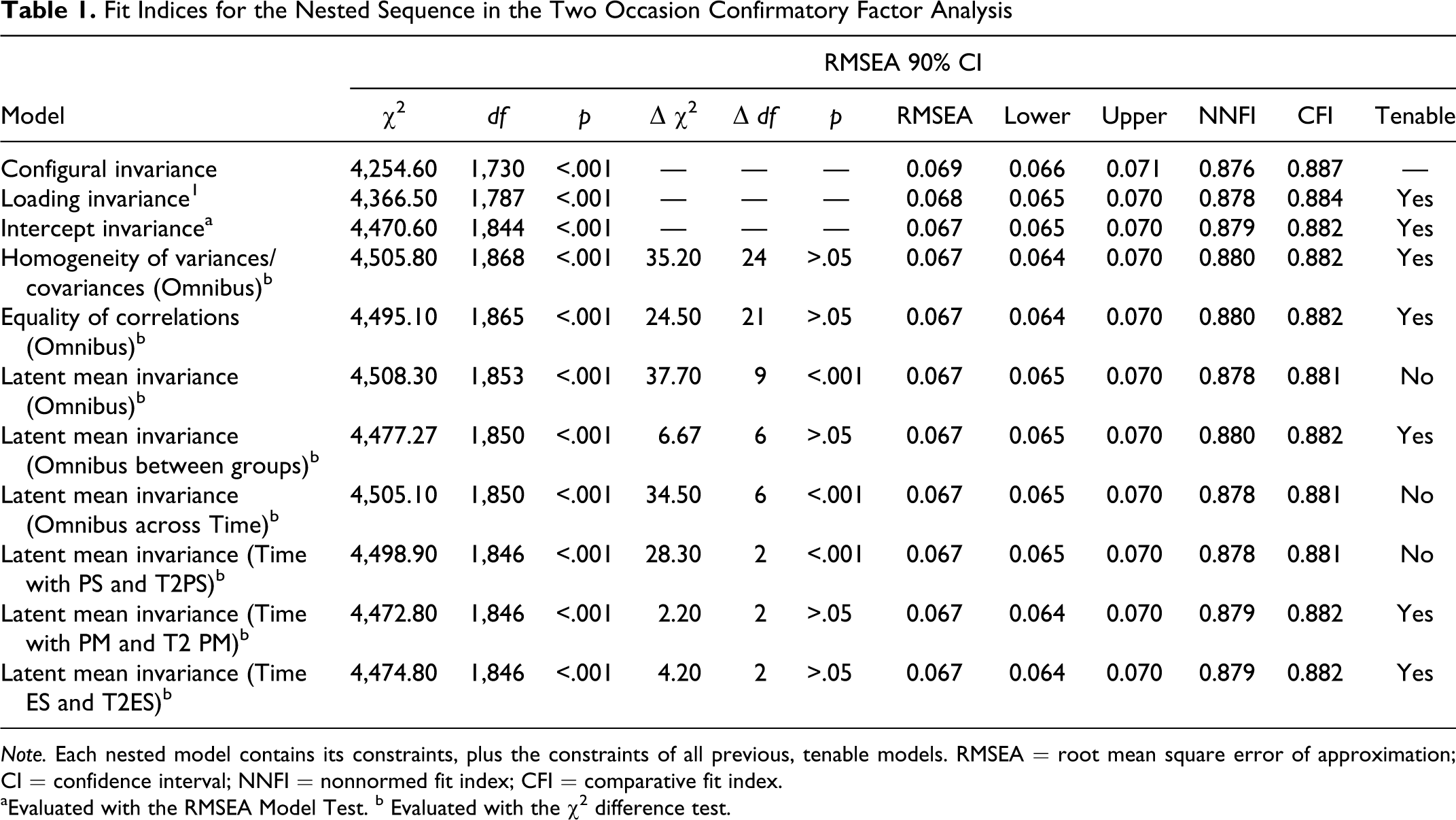
Note. Each nested model contains its constraints, plus the constraints of all previous, tenable models. RMSEA = root mean square error of approximation; CI = confidence interval; NNFI = nonnormed fit index; CFI = comparative fit index.

^aEvaluated with the RMSEA Model Test. ^b Evaluated with the χ²difference test.

In order to appropriately manage incomplete data, we used the multiple imputation technique (Enders, 2010; Graham, 2009; Graham, Cumsille, & Elek-Fisk, 2003; Graham, Taylor, Olchowski, & Cumsille, 2006). We used the SAS 9.2 MI procedure (PROC MI) with the Markov Chain Monte Carlo (MCMC) estimation to create 100 imputations (i.e., data sets) to retain optimal power (Collins, Schafer, & Kam, 2001; Graham et al., 2007; Schafer & Graham, 2002) under the assumptions of a missing at random (MAR) mechanism and multivariate normality. We determined that the imputed data sets should be separated by at least 40 iterations, so each data set was saved after a much more conservative 200 iterations. The imputation process included 42 variables (8 measures of parenting stress, 7 measures of personal mastery, and 7 measures of economic stress) and the account holders and nonaccount holders were imputed separately (Enders & Gottschall, 2011). After imputing all 100 data sets, we created a correlation table with means and standard deviations (Wu, Lang, & Little, 2009) that were used for subsequent analyses.

Analytical Procedures

A multiple group CFA was used to examine the measurement and structural properties (i.e., population heterogeneity) of the parenting stress, personal mastery, and economic strain measures across two measurement occasions and across both groups with the LISREL 8.80 statistical package (Jöreskog & Sörbom, 2007) using maximum likelihood. All model results are from converged, admissible solutions. Because it was hypothesized that invariance of the loadings and intercepts across the indicators of parenting stress, personal mastery, and economic strain through both measurement occasions and groups would be supported, factorial invariance was tested through the sequences recommended by Little and Colleagues (2007).

A multiple group CFA was used because it allows for the examination of observed and latent variables within a single measurement occasion or group as well as across repeated measures or multiple groups (Kline, 2010). A CFA is often referred to as a measurement model because it empirically tests a theoretical factor structure. In this procedure, many observed variables (i.e., indicators) are individually separated into common and specific variance. The common variance of an indicator is used to contribute to the definition of an unobserved (i.e., latent) variable, while the specific variance is regarded as measurement error and is removed from the definition of the latent construct (Brown, 2006). Therefore, a latent variable does not contain measurement error and can be used to greatly enhance the accuracy of associations and predictions because inferences are based only on true score variance. In addition to the ability to create and model latent variables, there are other benefits of CFA over other analytic techniques such as the ability to estimate multiple equations simultaneously, the capacity to assess the appropriateness of a specified model both within a population and across populations and occasions, as well as enormous flexibility in the specification of a theoretical model, including correlated residuals (Brown, 2006; Kline, 2010; Little et al., 2007; Rigdon, 1998).

Based on previous research (Okech, Little, Williams Shanks, & Adams, 2010), a three-factor (three latent variables measured at two occasions) measurement model was specified in which: “My family has enough money to afford the kind of home that we need” (ES1, T2ES1), “My family has enough money to afford the kind of clothes that we need” (ES2, T2ES2), “My family has enough money to afford the kind of furniture or household equipment that we need” (ES3, T2ES3), “My family has enough money to afford the kind of car that we need” (ES4, T2ES4), “My family has enough money to afford the kind of food that we need” (ES5, T2ES5), “My family has enough money to afford the kind of medical care that we need” (ES6, T2ES6), and “My family has enough money to afford the kind of leisure and recreational activities we need” (ES7, T2ES7) loaded on the latent variable of economic strain for the first and second measurement occasions, respectively, that is, T2 refers to the second measurement occasion.

Furthermore, the personal mastery latent variable was composed of the following manifest indicators measured at two occasions: “There is no way I can solve some of the problems I have” (PM1, T2PM1), “I feel that I am being pushed around in life” (PM2, T2PM2), “I have little control over the things that happen to me” (PM3, T2PM3), “I can do anything I set my mind to” (PM4, T2PM4), “I feel helpless in dealing with the problems of life” (PM5, T2PM5), “What happens to me in the future depends on me” (PM6, T2PM6), and “There is little I can do to change the important things in my life” (PM7, T2PM7).

Lastly, the latent variable of parenting stress was composed of the following indicators: “I am happy with my role as a parent” (PS1, T2PS1), “In my role as a parent/caregiver, I often find that I have too little time for myself” (PS2, T2PS2), “As a parent, I enjoy the time I spend with my child(ren)” (PS3, T2PS3), “I feel overwhelmed with responsibilities of being a parent” (PS4, T2PS4), “As a parent/caregiver, I am able to find a balance between the many demands for my time and energy” (PS5, T2PS5), “As a parent/caregiver, I often find that my life is much more work than pleasure” (PS6, T2PS6), “I am satisfied as a parent caregiver” (PS7, T2PS7), and “I often feel tired, worn out or exhausted by the responsibilities of being a parent/caregiver” (PS8, T2PS8).

Using the correlation table that was earlier created, SEM was used to test correlation among the constructs across groups and occasions. All latent variables were freely correlated. To set the scale for model estimation, we used the effects-coding method (Little, Slegers, & Card, 2006). The effects-coding technique allowed for “scaling that is in a meaningful metric; that is, a given latent variable will be on the same scale as the average of all its manifest indicators” (Little et al., 2006, p. 67). In other words, all the factor loadings are constrained to average 1 and all the indicator intercepts to sum to 0, resulting in the construct being in the same metric of the (weighted average) of all indicators (Little et al., 2007). This scale setting technique allowed for the estimation of latent variance in both measurement occasions and groups that was comparable and not arbitrarily set. This method was also utilized to set the scale for intercepts in order to assess the latent means in a comparable nonarbitrary metric.

Results

Invariance Testing

Initially, the patterns of fixed and free factor loadings for similarity (i.e., configural invariance) across measurement occasions and groups were assessed. This model contained no double-loading indicators, and all measurement error unrelated to repeated measurement was assumed to be uncorrelated. As expected, this model failed the chi-square exact fit test χ² (1730, N = 381) = 4254.60, p < .001 (see MacCallum & Browne, 1993; Reise et al., 1993; Rigdon, 1998). However, the value of the RMSEA was .069 and the 90% confidence interval was [.066, .071]. Moreover, the relative fit of the model was about 89% improvement over the fit of the independence model (CFI = .887). Likewise, the NNFI was .876. Taken together the model fit indices of this CFA suggest reasonable fit.

Next, the patterns of fixed and free factor loadings (Λ) for equivalence (i.e., weak invariance) across groups and occasions were assessed. This test assesses whether the latent constructs are set up the same way among account holders and nonaccount holders at both measurement occasions and if the latent constructs have the same meaning (Brown, 2006). As noted in Table 1, we found no significant changes in model fit for the omnibus test across groups and measurement occasions. These results suggest that the indicator loadings are comparable across time and group. More specifically, change in an indicator will relate to change in the latent variable that is essentially identical across groups and across occasions.

We then evaluated the equivalence of the indicator means simultaneously across both measurement occasions and groups (i.e., strong invariance). The omnibus test of strong invariance across time and groups was not significant (see Table 1). These results suggest that at a given level of parenting stress, personal mastery, and economic strain participants with and without an account measured at both occasions would have the same observed scores on an indicator. This suggests that the constructs have the same meaning across groups and across occasions.

Parameter Interpretation—Reliability, Convergent, and Discriminant Validity

Table 2 contains the loadings, intercepts, residuals, and squared multiple correlations ([SMCs] R ²) for each indicator, as well as the latent variance. The direction of the parameter estimates was as expected, PS1-T2PS8 positively loaded on the parenting stress latent factor, PM1-T2PM7 positively loaded on the personal mastery latent factor, and ES1-T2ES7 positively loaded on the economic strain latent factor. All freely estimated factor variances, loadings, and residual errors were not out of bounds and significantly differed from 0 (Wald test; p < .05). More specifically, all measured variables that were expected to measure a common factor had relatively high standardized loadings (see Table 2) on that factor; which provides evidence of convergent validity. In other words, different indicators of the distinct constructs in this study were strongly related with their respective constructs. Additionally, the parenting stress, personal mastery, and economic strain factors were not collinear (i.e., the latent correlation was < .90); which suggests discriminant validity. In other words, indicators of the distinct constructs in this study were not highly intercorrelated to suggest that either of the constructs had been erroneously into two or more factors (Brown, 2006). Likewise, the latent factors measured at the first measurement occasion were not collinear with the latent factors at the second measurement occasion, which suggests that enough time passed between measurement occasions.

Table 2.

Loading and Intercept Values, Residuals, and R² Values for Each Indicator, and the Estimated Latent Variance from the Strong Metric Invariance Model

		Equated estimates			Standardized		Account holders		Nonaccount
Indicator	Loading	Std. Err.	Intercept	Std. Err.	Loading^a	Intercept^a	Theta	R ²	Theta	R ²
Parental stress Time 1 (PS): Estimated latent variance (account = .12; no account = .09)
PS1	0.63	0.05	0.05	0.09	0.44	0.10	0.20	0.185	0.18	0.17
PS2	1.24	0.07	0.37	0.15	0.50	0.45	0.51	0.257	0.57	0.20
PS3	0.49	0.04	0.23	0.08	0.38	0.53	0.16	0.148	0.15	0.13
PS4	1.61	0.07	−1.01	0.14	0.65	−1.20	0.41	0.421	0.48	0.33
PS5	0.71	0.06	0.55	0.12	0.38	0.88	0.38	0.132	0.29	0.14
PS6	1.15	0.07	0.33	0.14	0.48	0.40	0.54	0.221	0.56	0.18
PS7	0.83	0.05	−0.18	0.10	0.51	−0.32	0.26	0.237	0.17	0.27
PS8	1.35	0.06	−0.35	0.13	0.60	−0.45	0.36	0.367	0.48	0.26
Personal mastery Time 1 (PM): Estimated latent variance (account = .19; no account = .19)
PM1	1.03	0.05	0.35	0.09	0.52	0.41	0.56	0.267	0.46	0.32
PM2	1.15	0.04	−0.28	0.07	0.70	−0.39	0.29	0.471	0.22	0.54
PM3	1.16	0.04	−0.26	0.07	0.68	−0.34	0.33	0.442	0.27	0.50
PM4	0.68	0.04	0.29	0.07	0.49	0.47	0.30	0.227	0.23	0.29
PM5	1.21	0.04	−0.35	0.07	0.73	−0.48	0.27	0.508	0.22	0.58
PM6	0.65	0.04	0.39	0.07	0.45	0.62	0.35	0.189	0.26	0.24
PM7	1.12	0.04	−0.14	0.08	0.63	−0.18	0.41	0.372	0.28	0.47
Economic strain Time 1 (ES): Estimated latent variance (account = .41; no account = .35)
ES1	1.05	0.03	−0.35	0.09	0.68	−0.38	0.49	0.456	0.49	0.42
ES2	1.16	0.02	−0.28	0.06	0.84	−0.33	0.25	0.668	0.20	0.68
ES3	1.21	0.02	−0.50	0.06	0.88	−0.59	0.16	0.77	0.21	0.69
ES4	1.05	0.03	−0.25	0.08	0.74	−0.28	0.37	0.529	0.37	0.49
ES5	0.68	0.03	1.28	0.07	0.67	2.05	0.31	0.364	0.18	0.45
ES6	0.84	0.04	0.41	0.09	0.59	0.47	0.50	0.347	0.54	0.29
ES7	1.02	0.03	−0.32	0.07	0.77	−0.38	0.30	0.572	0.27	0.56
Parental stress Time 2 (T2PS): Estimated latent variance (account = .11; no account = .06)
T2PS1	0.63	0.05	0.05	0.09	0.44	0.10	0.17	0.215	0.26	0.09
T2PS2	1.24	0.07	0.37	0.15	0.49	0.44	0.57	0.236	0.66	0.13
T2PS3	0.49	0.04	0.23	0.08	0.41	0.57	0.12	0.193	0.22	0.06
T2PS4	1.61	0.07	-1.01	0.14	0.65	−1.19	0.41	0.425	0.55	0.23
T2PS5	0.71	0.06	0.55	0.12	0.38	0.86	0.37	0.135	0.32	0.09
T2PS6	1.15	0.07	0.33	0.14	0.45	0.38	0.54	0.221	0.82	0.09
T2PS7	0.83	0.05	−0.18	0.10	0.55	−0.35	0.21	0.276	0.22	0.16
T2PS8	1.35	0.06	−0.35	0.13	0.61	−0.46	0.34	0.383	0.47	0.20
Personal mastery Time 2 (T2 PM): Estimated latent variance (account = .20; no account = .23)
T2PM1	1.03	0.05	0.35	0.09	0.54	0.42	0.59	0.257	0.51	0.29
T2PM2	1.15	0.04	−0.28	0.07	0.71	−0.39	0.30	0.469	0.27	0.50
T2PM3	1.16	0.04	−0.26	0.07	0.66	−0.33	0.37	0.413	0.35	0.43
T2PM4	0.68	0.04	0.29	0.07	0.49	0.47	0.30	0.231	0.24	0.27
T2PM5	1.21	0.04	−0.35	0.07	0.74	−0.48	0.22	0.571	0.31	0.48
T2PM6	0.65	0.04	0.39	0.07	0.46	0.63	0.30	0.216	0.34	0.20
T2PM7	1.12	0.04	−0.14	0.08	0.61	−0.17	0.42	0.365	0.43	0.37
Economic strain Time 2 (T2ES): Estimated latent variance (account = .43; no account = .55)
T2ES1	1.05	0.03	−0.35	0.09	0.63	−0.38	0.51	0.404	0.56	0.39
T2ES2	1.16	0.02	−0.28	0.06	0.83	−0.36	0.19	0.694	0.19	0.70
T2ES3	1.21	0.02	−0.50	0.06	0.86	−0.63	0.17	0.729	0.21	0.69
T2ES4	1.05	0.03	−0.25	0.08	0.71	-0.30	0.38	0.479	0.33	0.52
T2ES5	0.68	0.03	1.28	0.07	0.57	1.92	0.29	0.334	0.29	0.34
T2ES6	0.84	0.04	0.41	0.09	0.54	0.47	0.52	0.299	0.51	0.31
T2ES7	1.02	0.03	−0.32	0.07	0.70	−0.39	0.39	0.461	0.32	0.52

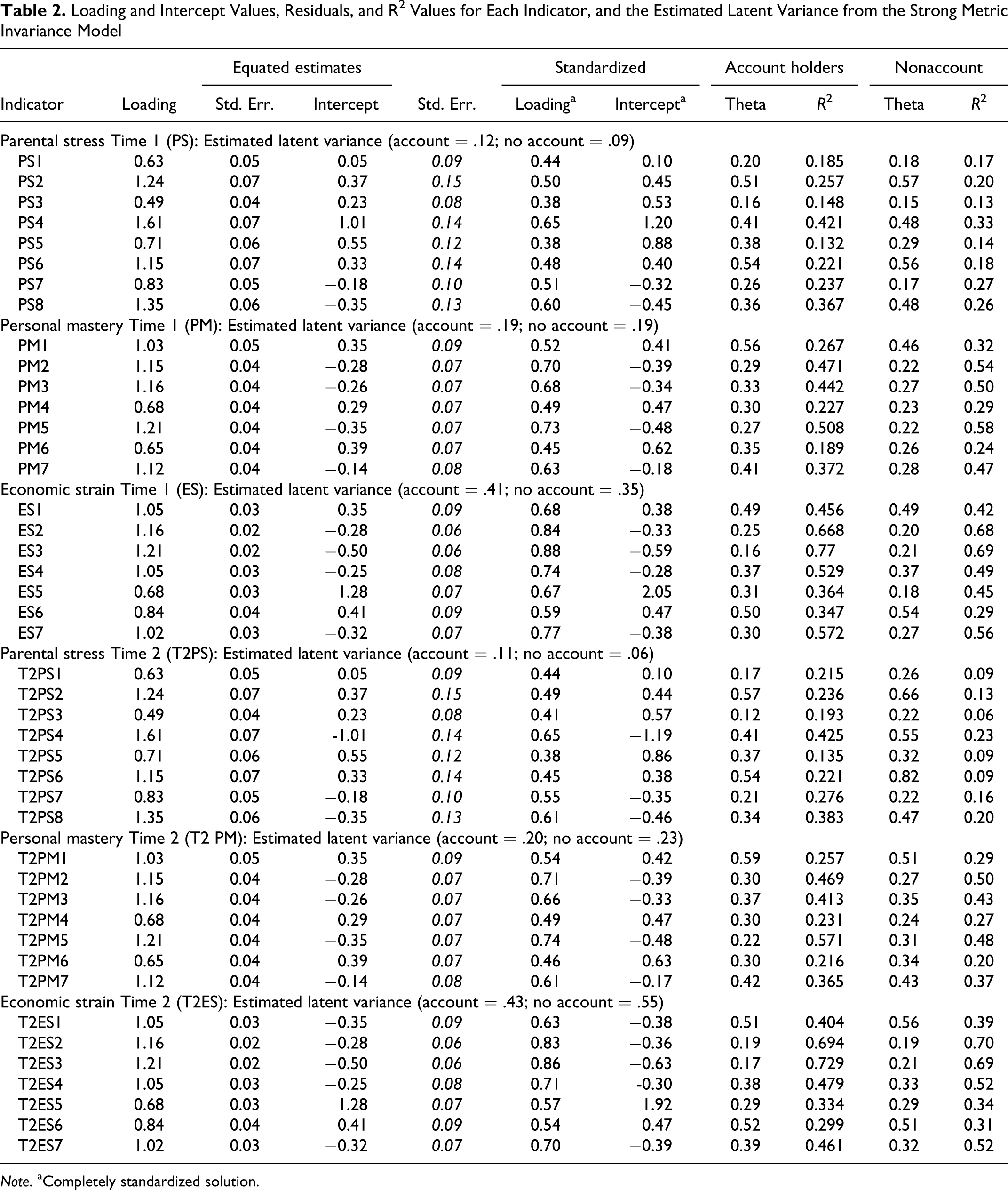
Note. ^aCompletely standardized solution.

The unstandardized loadings in Table 2 can be interpreted as regression coefficients of the latent variable predicting the associated measured variables. For example, the unstandardized factor loading for PS1 (i.e., I am happy with my role as a parent) is 0.63 (equated across time and group), which suggests that a 1-unit increase in the parenting stress factor is associated with a 0.63 unit increase in the PS1 measured variable. The completely standardized loadings (the latent factors and the manifest indicators are both standardized) can be interpreted as a correlation between the latent factor and the measured variable. For instance, the standardized factor loading for PS1 is 0.44 (equated across groups and across occasions). As a result, a standard deviation increase in the parenting stress factor is associated with a 0.44 standard deviation increase in the PS1 variable.

Additionally, reliability of the manifest indicators was assessed with SMCs (i.e. squared standardized factor loadings). SMCs can be interpreted as the percentage of variance in the measured variable that is accounted for by the latent factor. For example, 0.19 suggests that about 20% of the variance in PS1 is accounted for by parenting stress among participants that are account holders (see Table 2). Said differently, about 80% of the variance in “I am happy with my role as a parent” is not related to parenting stress. Table 2 also presents R ² values for each manifest variable by group and time. While some indicators were strongly related to the associated latent factor, other indicators were weak (R ² = .06–.77).

Scale reliability was assessed with the composite reliability for congeneric measures model (CRCMM; see Raykov, 1997) method. The CRCMM scale reliability estimates can be interpreted in the same manner as Cronbach’s α. Because the CRCMM method does not assume equal factor loadings, it is a better lower bound estimate of reliability than Cronbach’s α (Raykov, 1997). Among participants that were account holders, the CRCMM composite reliability index was .72 and .67 for the parenting stress indicators at the first and second measurement occasions, respectively; .69 and .71 for the personal mastery indicators at the first and second measurement occasion, respectively; and .83 and .85 for the economic strain indicators at the first and second measurement occasion, respectively. Among participants that were nonaccount holders, the CRCMM composite reliability index was .67 and .53 for the parenting stress indicators at the first and second measurement occasion, respectively; .85 and .69 for the personal mastery indicators at the first and second measurement occasion, respectively; and .87 and .88 for the economic strain indicators at the first and second measurement occasion, respectively. These results suggest that overall the scales are reliable because the items have a relatively high internal consistency.

Homogeneity of Variances and Covariance

Our second research question asked what the patterns of interrelationships are among the parenting stress, personal mastery, and economic strain factors across groups and across occasions. The establishment of factorial invariance allowed for further testing of latent parameters (i.e., population heterogeneity). As noted in Table 1, the omnibus test of both equal variances and covariances across time and group (account holder, nonaccount holder) was not significant, Δχ² (24, n = 381) = 35.20, p > .05, indicating that parenting stress, personal mastery, and economic strain did not differ across either measurement occasion or group membership. That is, the latent variance did not become more or less heterogeneous at the second measurement occasion or across groups. Therefore, no follow-up tests of latent variance and/or correlation differences were needed (see Table 1). The latent correlation matrix was generated using phantom constructs (Little et al., 2007) and is noted in Table 3. Phantom constructs were used to separate latent variances from latent correlations. More specifically, the phantom constructs were used to transform the variances of the three latent constructs into standard deviations and the covariance between them into a correlation (see Little et al., 2006). Phantom constructs have no substantive meaning and no disturbances but are created to force constraints on the model.

Table 3.

Correlations, Means, and Standard Deviations Between Latent Constructs for Both Measurement Occasions

	PS	PM	ES	T2PS	T2PM	T2ES
PS	1.00
PM	0.60	1.00
ES	−0.28	−0.13	1.00
T2PS	0.51	0.41	−0.22	1.00
T2 PM	0.34	0.53	−0.12	0.58	1.00
T2ES	−0.25	−0.08	0.50	−0.32	−0.21	1.00
Means	2.02	1.79	2.48	1.93	1.77	2.47
Std. dev.	0.34	0.44	0.59	0.34	0.44	0.59

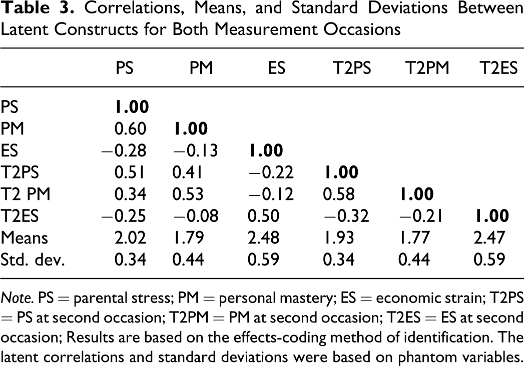
Note. PS = parental stress; PM = personal mastery; ES = economic strain; T2PS = PS at second occasion; T2PM = PM at second occasion; T2ES = ES at second occasion; Results are based on the effects-coding method of identification. The latent correlations and standard deviations were based on phantom variables.

The latent variance/covariance matrix is reported in Table 3 and illustrates that parenting stress and personal mastery correlate around .60 within each measurement occasion; parenting stress and economic strain correlate around −.30 within each measurement occasion; and personal mastery and economic strain correlate around −.14 within each measurement occasion. The stability correlations of the constructs over time are .52 and .50 (account holders and nonaccount holders, respectively) for parenting stress, .55 and .46 for personal mastery, and.49 and .45 for economic strain. Therefore, only about 27% of the variance in parenting stress remains stable from the first measurement occasion to the second among participants that are account holders and 25% among nonaccount holders. Likewise, about 30% of the variance in personal mastery remains stable from the first measurement occasion to the second among participants that are account holders and 21% among nonaccount holders. Lastly, only about 24% of the variance in economic strain remains stable from the first measurement occasion to the second among participants that are account holders and 20% among nonaccount holders.

Latent mean invariance

The next research question asked whether the groups differed in their average levels (i.e., means) of parenting stress, personal mastery, and economic strain. That is, we hypothesized that the degree of parenting stress, personal mastery, and economic strain were not stronger in either the first or second measurement occasion. As noted in Table 3 the latent means of parenting stress, personal mastery, and economic strain were not invariant, Δχ² (3, n = 381) = 37.70, p < .001, across time and group. These results suggest that the hypothesis of mean equivalence across time and group in the population is rejected. That is, at least one of the three latent means changed over time, between groups or both. The latent means and standard deviations are included in Table 3. Follow-up tests indicated evidence for a main effect of time relating to parenting stress. The latent mean of parenting stress at the first measurement occasion (M = 2.02, SD = 0.34) was significantly different, Δχ² (2, n = 381) = 28.30, p < .001, (at the .017 level; Bonferroni correction) from the latent mean of parenting stress at the second measurement occasion (M = 1.93, SD = 0.34). All other latent means did not significantly change over time (see Table 2). The latent effect size was in the small-to-medium range (d = .25). There were no group differences in the means or interactions between group and time.

Discussion and Application to Social Work

Tests of Invariance

The purpose of this study was to determine whether parenting stress, personal mastery, and economic strain were the same constructs across both measurement occasions and groups. The results suggest that there is no significant difference in the measurement properties of these constructs across the time frame investigated, which provides evidence of construct validity and allowed for tests of population heterogeneity. Findings show that the measurement variability did not change between the first and second measurement occasions. Also, the variance of economic strain increased from the first to the second measurement occasion and a group membership did not have a heterogeneous effect on the increased variance in economic strain. A mean difference was observed between parenting stress at the first and second measurement occasion. Given these results, it was concluded that participants on average reported more parenting stress at the first measurement occasion than at the second occasion. That is, at baseline, the variances were more homogeneous because individuals were more similar with regard to their level of parenting stress.

Reliability of the Manifest Indicators

Many of the relationships between the latent factors and associated individual items did not appear to be large (i.e., less than 50% of the variance explained, see Table 2); however, some indicators contributed a large amount of variance. The most reliable indicator of parenting stress at both measurement occasions was PS4 (I feel overwhelmed with responsibilities of being a parent.). The least reliable indicator at both measurement occasions was PS3 (As a parent, I enjoy the time I spend with my children.) The most reliable indicator of personal mastery at both measurement occasions was PM5 (I feel helpless in dealing with the problems of life.). The least reliable at both measurement occasions was PM6 (There is little I can do to change the important things in my life.). The most reliable indicator of economic strain at both measurement occasions was ES3 (My family has enough money to afford the kind of furniture or household equipment that we need.). The least reliable at both measurement occasions was ES5 (My family has enough money to afford the kind of food that we need.). The low reliability estimates of some items are not particularly concerning because item level data are notoriously prone to low reliability (see Little, Cunningham, & Shahar, 2002). Additionally, the CRCMM composite reliability index demonstrated good scale reliability among the manifest indicators.

The article reported here focused on the measurement properties of the manifest and latent constructs as well as the analytical techniques that are applicable to multiple-group multiple occasions MACS. For a presentation of the policy and program implications of these results in asset building and the future well-being of children who have child development accounts, see a separate article (Okech, 2012, Research on Social Work Practice). The article was built on the call by Guo and colleagues (2009) in applying appropriate SEM procedures that may strengthen and encourage the use of SEM in social work research. It is hoped that this will indeed become a secondary outcome of this article.

Application to Social Work

Guo and colleagues (2009) noted the following as best practices in SEM reporting: (1) a theoretical specification; (2) consideration of alternative models; (3) reporting method of estimation; (4) an adequate sample size; (5) application of the appropriate model fits; (6) use of model specification where applicable, and (7) reporting of sufficient information that may allow evaluation and replication. Clearly, the article reported here adhered to these best practices and also included information on item reliability and validity that is important for social work research. Since a number of the concepts that social workers deal with have multiple dimensions (Rubin & Babbie, 2011), ensuring that the items are highly correlated with their respective constructs is important in ensuring the validity and reliability of the constructs of interest. As recommended by Guo and colleagues (2009), the article presented here also provides sufficient attention to how missing data were handled and how univariate and multivariate normality were examined.

In conclusion, the use of SEM methods by social workers is likely to increase in the future. The advantages and strengths of the technique are better than path analysis or ordinary least squares regression since SEM and CFA methods account for errors in the variables of interest. There is need for social work doctoral programs to offer courses in the subject. Social work doctoral students may, however, take SEM courses in other departments that are currently more likely to offer the courses, including psychology, business, or education. The best practices suggested by Guo and colleagues (2009) as well as the step-by-step methods specified by Little and colleagues (2007) are user-friendly and basic for beginners in SEM methods.

Footnotes

Authors’ Note

The correlation items tables with means and standard deviations that may be used for replicating the findings presented here are available upon request from the author. Deborah Adams, Associate Professor at the University of Kansas School of Social Welfare and SEED research principal investigator has always provided invaluable help in understanding asset building programming and policy design. Finally, the author thanks colleagues at the University of Kansas, Department of Quantitative Psychology including Professor Todd D. Little, Director, Center for Research and Data Analysis and Mr. Waylon J. Howard for help in applying SEM methods in a systematic manner.

I am thankful for the two anonymous reviewers who offered helpful critiques to the original manuscript and for the encouragement to submit a purely measurement paper.

This article is a breakout from a separate one (accepted for publication in this journal) that focused mostly on the implications for practice and policy. A figure showing the flow of participants can also be found in the breakout article in this journal.

Declaration of Conflicting Interests

The author declared no potential conflicts of interest with respect to the research, authorship, and/or publication of this article.

Funding

Saving for Education, Entrepreneurship, and Downpayment (SEED) is a policy, practice, and research initiative designed to test the efficacy of and inform policy for a national system of asset-building accounts for children and youth. SEED is led by six national partners: CFED, the Center for Social Development at Washington University in St. Louis, the University of Kansas (KU) School of Social Welfare,the New America Foundation, the Initiative on Financial Security of the Aspen Institute, and RTI International. Support for the SEED initiative is funded by the Ford Foundation, Charles and Helen Schwab Foundation, Jim Casey Youth Opportunity Initiative, Citigroup Foundation, Ewing Marion Kauffman Foundation, Charles Steward Mott Foundation, Richard and Rhoda Goldman Fund, MetLife Foundation, Evelyn and Walter Haas, Jr. Fund, Lumina Foundation for Education and the Edwin Gould Foundation for Children.

References

Abidin

. (1992). The determinants of parenting behavior. Journal of Clinical Child Psychology, 21, 407–412. Retrieved from http://www.jccap.net

Adams

(2008). SEED Pre-School Demonstration and Impact Assessment. Research Brief, SEED Research at KU. Lawrence, KS: University of Kansas School of Social Welfare.

Adams

Williams Shanks

T. R.

Marks

(2008). SEED Pre-School Demonstration and Impact Assessment: Findings to Date. Research Brief, SEED Research at KU. Lawrence, KS: University of Kansas School of Social Welfare.

Bentler

P. M.

(1990). Comparative fit indexes in structural models. Psychological Bulletin, 107, 238–246.

Bentler

P. M.

Bonett

D. G.

(1980). Significance tests and goodness of fit in the analysis of covariance structures. Psychological Bulletin, 88, 588–606.

Berry

J. O.

Jones

W. H.

(1995). The parental stress scale: Initial psychometric evidence. Journal of Social and Personal Relationships, 12, 463–472. doi: 10.1177/0265407595123009

Beverly

S. G.

Williams

Shanks T.

(2005). SEED Impact Assessment Survey: baseline Instrument in English and Spanish. Research Instrument, SEED Research at KU. Lawrence, KS: University of Kansas School of Social Welfare.

Bodner

T. E.

(2007). Review of Missing data and small-area estimation: Modern analytical equipment for the survey statistician. Psychometrika, 72, 115–116.

Bollen

K. A.

Curran

P. J.

(2004). Autogressive latent trajectory (ALT) models. Av synthesis of two traditions. Sociological Methods and Research, 32, 336–387.

10.

Brown

T. A.

(2006). Confirmatory factor analysis for applied research. New York, NY: The Guilford Press.

11.

Browne

M. W.

Cudeck

(1993). Alternative ways of assessing model fit. In K. A. B. J. S. Long (Ed.), Testing structural equation models (pp. 136–162). Newbury Park, CA: Sage.

12.

Carter

R. L.

(2006). Solutions for missing data in structural equation modeling. Research & Practice in Assessment, 1, 1–6.

13.

Cheung

G. W.

Rensvold

R. B.

(2002). Evaluating goodness-of-fit indexes for testing measurement invariance. Structural Equation Modeling, 9, 233–255.

14.

Cohen

. (1988). Statistical power analysis for the behavioral sciences. Lawrence Erlbaum.

15.

Collins

L. M.

Schafer

J. L.

Kam

C. M.

(2001). A comparison of inclusive and restrictive strategies in modern missing data procedures. Psychological methods, 6, 330–351.

16.

Conger

R. D.

Conger

K. J

. (2002). Resilience in Midwestern families: Selected Findings from the first decade of a prospective, longitudinal study. Journal of Marriage and the Family, 64, 361–373. doi:10.1111/j.1741-3737.2002.00361.x

17.

Conger

R. D.

X. J.

Elder

G. H.

Jr Lorenz

F. O.

Simons

R. L

. (1994). Economic stress, coercive family process, and developmental problems of adolescents. Child Development, 65, 541–561. doi:10.111/j.1467-8624.1994.tb00768.x

18.

Conger

R. D.

Wallace

L. E.

Sun

Simons

R. L.

McLoyd

V. C.

Brody

G.H

. (2002). Economic pressure in African American families: A replication and extension of the family stress model. Developmental Psychology, 38, 179–193. doi:10.1037//0012-1649.38.2.179

19.

Curley

Sherraden

(2000). Policy lessons from children’s savings accounts. Child Welfare, 79, 661–687.

20.

Enders

C. K.

(2006). A primer on the use of modern missing data methods in psychosomatic medicine research. Psychosomatic Medicine, 68, 427–736.

21.

Enders

C. K.

(2010). Applied missing data analysis. New York, NY: Guilford Press.

22.

Enders

C. K.

Bandalos

D. L.

(2001). The relative performance of full information maximum likelihood estimation for missing data in structural equation models. Structural Equation Modeling, 8, 430–457.

23.

Enders

C. K.

Gottschall

A. C.

(2011). Multiple imputation strategies for multiple group structural equation models. Structural Equation Modeling: A Multidisciplinary Journal, 18, 35–54.

24.

Graham

J. W.

(2009). Missing data analysis: Making it work in the real world. Annual Review of Psychology, 60, 549–576.

25.

Graham

J. W.

Cumsille

P. E.

Elek-Fisk

(2003). Methods for handling missing data (Vol. 2). New York, NY: Wiley.

26.

Graham

J. W.

Olchowski

A. E.

Gilreath

T. D.

(2007). How many imputations are really needed? Some practical clarifications of multiple imputation theory. Prevention Science, 8, 206–213.

27.

Graham

J. W.

Taylor

B. J.

Olchowski

A. E.

Cumsille

P. E.

(2006). Planned missing data designs in psychological research. Psychological Methods, 11, 323–343.

28.

Guo

Perron

B. E.

Gillespie

D. F.

(2009). A systematic review of structural equation modeling in social work research. British Journal of Social Work, 39, 1556–1574. doi:10.1093/bjsw/bcn101

29.

Bentler

P. M

. (1999). Cut off criteria for fit indexes in covariance structure analysis. Structural Equation Modeling, 6, 1–55

30.

Jöreskog

K. G.

Sörbom

(2007). LISREL 8.80. Chicago, IL: Scientific Software International.

31.

Kline

(1998). Principles and practice of structural equation modeling. New York: The Guilford Press.

32.

Kline

(2005). Principles and practice of structural equation modeling. New York: The Guilford Press.

33.

Kline

(2010). Principles and practice of structural equation modeling. New York, NY: The Guilford Press.

34.

Little

(1997). Mean and covariance structures (MACS) analyses of cross-cultural data: Practical and theoretical issues. Multivariate Behavioral Research, 32, 53–76.

35.

Little

T. D.

Card

N. A.

Sledgers

D. W.

Ledford

E. C.

(2007). Representing contextual effects in multiple-group MACS models. In Little

T. D.

Bovaird

J. A.

Card

N. A.

(Eds.), Modeling contextual effects in longitudinal studies (pp. 121–147). Mahwah, NJ: Lawrence Erlbaum Associates.

36.

Little

T. D.

Cunningham

W. A.

Shahar

(2002). To parcel or not to parcel: Exploring the question, weighing the merits. Structural Equation Modeling, 9, 151–173.

37.

Little

T. D.

Slegers

D. W.

Card

N. A.

(2006). A non-arbitrary method of identifying and scaling latent variables in SEM and MACS models. Structural Equation Modeling, 13, 59–72.

38.

MacCallum

R. C.

Browne

M. W.

(1993). The use of casual indicators in covariance structure models: Some practical issues. Psychological Bulletin, 114, 533–541.

39.

Marks

Rhodes

(2005). Saving for education, entrepreneurship and downpayment wave 1 survey—Fall 2004. Research Triangle Park, North Carolina: RTI International.

40.

Meredith

(1993). Measurement invariance, factor analysis and factorial invariance. Psychometrika, 58, 525–543.

41.

Morrison

D. R.

Zaslow

M. J.

Dion

M. R.

(1998). Completing the portrayal of parenting: Behavior with survey measures of parenting. In Zaslow

Eldred

(Eds.), Parenting behavior in a sample of young mothers in poverty: Results of the New Chance Observational Stud (pp. 25–53). New York, NY: Manpower Demonstration Research Corporation.

42.

Okech

. (2012). Evaluating the effects of child savings accounts program participation on parental well-being. Research on Social Work Practice, 22 (4), 357–366.

43.

Okech

Little

T. D.

Williams Shanks

T. R.

Adams

(2011). Self-efficacy and joining a savings program for children’s education. Research on Social Work Practice, 21, 442–451. doi:10.1177/1049731510389079

44.

Pearlin

L. I.

Schooler

(1978). The structure of coping. Journal of Health and social behavior, 9(1), 2–21. Retrieved from http://www.jstor.org/stable/2136319.

45.

Raykov

(1997). Scale reliability, Cronbach's coefficient alpha, and violations of essential tau-equivalence with fixed congeneric components. Multivariate Behavioral Research, 33, 343–363.

46.

Reise

S. P.

Widaman

K. F.

Pugh

R. H.

(1993). Confirmatory factor analysis and item response theory: two approaches for exploring measurement invariance. Psychological Bulletin, 114, 552–566.

47.

Rigdon

E. E

. (1998). Structural equation modeling. In Marcoulides

G. A.

(Ed.), Modern methods for business research (pp. 251–294). Mahwah, NJ: Lawrence Erlbaum.

48.

Rubin

Babbie

(2011). Research methods for social work (7th ed.). Belmont, CA: Thomson Brooks/Cole.

49.

Schafer

J. L.

Graham

J. W.

(2002). Missing data: Our view of the state of the art. Psychological Methods, 7, 147–177.

50.

Schafer

J. L.

Olsen

M. K.

(1998). Multiple imputation for multivariate missing-data problems: A data analyst's perspective. Multivariate Behavioral Research. Special Issue: Innovative Methods for Prevention Research, 33, 545–571.

51.

Sherraden

(1991). Assets and the poor: A new American welfare policy. Armonk, NY: M.E. Sharpe, Inc.

52.

Steiger

(1990). Structural model evaluation and modification: An interval estimation approach. Multivariate Behavioral Research, 25, 173–180.

53.

Widaman

K. F.

Reise

S. P.

(1997). Exploring the measurement invariance of psychological instruments: Applications in the substance use domain. In Bryant

K. J.

Windle

S. G.

West

(Eds.), The science of prevention: Methodological advances from alcohol and substance abuse research (pp. 281–324). Washington, DC: American Psychological Association.

54.

Lang

K. M.

Little

T. D.

(2009). Does it fit? A simple method of assessing model fit and testing significance in multiply imputed data. Paper presented at the Society for Multivariate Experimental Psychology, Shalishan , Oregon.