Electoral Turnout and State Redistribution

Individual-level Turnout

One basic way of measuring turnout is at the individual level. Individual-level data on electoral participation are derived from the surveys that are conducted in many countries at the time of national elections, which invariably ask respondents whether they voted in the election in question. Again, the most important advantage of election studies is that they offer information about respondents’ household income—information that is obviously not available in national-level aggregate data on turnout.

Despite this advantage, electoral studies have a disadvantage that limits their usefulness in comparative work: self-reported data almost always indicate a higher rate of turnout than data from national electoral rolls, which are based on actual election results. To make matters worse, the extent of overreporting varies considerably from country to country. A good deal of attention has been paid to the overreporting problem in the scholarly literature, particularly with reference to the American National Election Studies (ANES, 2013). The consensus is that the most important reason for overreporting is a tendency for some respondents to seek social approval by telling interviewers that they voted in a given election even if they did not actually do so (Karp and Brockington 2005; Katz and Katz 2010, 824–25; McDonald 2003, 2007). ¹

National-level Average Turnout

A first goal of this article is to reconcile individual-level data—which are, of course, the only data offering information on eligible voters’ income—with national-level aggregate data. In this section, we will introduce the aggregate-level data on turnout in national elections that will be employed in this effort.

As has been suggested, there are two basic approaches to measuring electoral turnout at the national level; in one, the denominator is the registered population and in the other, it is the voting-age population (VAP). Cross-national studies employing the former approach include Franklin (2004) and Blais and Dobrzynska (1998); studies employing the latter include Endersby and Krieckhaus (2008) and Gray and Caul (2000). In both measures, the numerator of the turnout ratio is the same: the number of votes recorded by national electoral authorities. Although there is ordinarily no alternative to these figures, there are some possible concerns even in the straightforward matter of measuring how many people voted in a given election. For one thing, procedures vary in assessing ballots that are invalid because voters did not follow electoral rules or because their intentions were unclear. When possible, we count such votes (the number of which is ordinarily very small). And, of course, votes can be misreported, whether intentionally or unintentionally, although in most modern democracies there are extensive safeguards against errors or electoral manipulation. Despite these practical concerns, the consensus is that the vote totals reported by electoral authorities in the developed countries are very similar to the number of ballots actually cast, similar enough to have only a miniscule effect on national averages. In the words of Franklin (2004, 86) “this number is as near to being cross-nationally comparable as any statistic in comparative political research.”

There is no such consensus concerning the denominator of the turnout ratio. The most obvious choice would seem to be the registered electorate, the list of persons who have been legally certified as eligible to vote in a country. Such a figure, however, depends not only on the accuracy of electoral rolls but also, especially, on the share of the eligible population that is registered. In a large majority of developed democracies, the onus of registration is on the state, which takes responsibility for maintaining and updating registration rolls. One or the other (sometimes both) of two basic methods is employed: eligible citizens are obliged by law to register or the state compiles registration lists from such sources as national identity registers, tax rolls, vehicle license lists, military service registers, and social benefit recipient lists. ² Maintenance of up-to-date and accurate electoral rolls is ordinarily accompanied by a mechanism whereby would-be voters who do not appear on electoral registers can verify their eligibility at the time of the election.

In most of the countries included in this analysis, then, the ultimate responsibility for registration rests with the state, not the individual, and electoral authorities are mandated to ensure that all eligible persons are registered. The one glaring exception is the United States, where registration is entirely the responsibility of the individual. Even when registered voters do no more than change their residence, they must typically take the initiative to reregister at their new address, and if they move to another state, they may be faced with an entirely different registration process. Moreover, in most U.S. states, potential voters must register in advance of an election—most commonly thirty days in advance. For these and other reasons, a substantial share of eligible voters in the United States remains unregistered, in some cases for their entire lives.

Before the twenty-first century, the standard solution to the obvious inadequacy of vote/registered figures for the United States was to express turnout relative to the VAP. However, when McDonald and Popkin (2001) looked more closely at VAP figures for the United States, they found that, not only did they include a good many ineligibles but also, the number of ineligibles had grown steadily over time. The most important reason for this was a growing number of resident noncitizens in the U.S. voting-age population. In addition, U.S. voting law disqualifies persons who are incarcerated as well as, in many states, persons on parole or probation and even, in a few states, persons who had committed a felony in the past but had long since served their prison terms. McDonald (2012) excludes such persons from the denominator of U.S. turnout figures and also adds a much smaller number of U.S. citizens living abroad, who had previously not been counted. His are the figures that will be employed in this article.

One more issue must be briefly considered. The numerator of turnout figures ordinarily focuses on votes for the lower house of a country’s legislature, which in parliamentary systems produces the executive. However, in the United States, Finland, Austria, and Ireland, presidents and legislatures are separately elected by popular vote. For the United States, we have focused on turnout in presidential elections, which unambiguously produce the executive. ³ A less obvious case is Finland, in which a separately elected president serves alongside the prime minister. However, since the 2000 constitution and 2012 amendments to it, the position of president has been less powerful than that of the prime minister, particularly in the domestic arena (Ministry of Foreign Affairs of Finland 2013). We have thus focused on turnout in Finnish parliamentary elections. Finally, in Austria and Ireland, the presidency, while directly elected, is primarily a symbolic position, so we have focused on legislative elections in these cases.

To summarize, we have used McDonald’s voting-eligible figures as the denominator of U.S. turnout figures, and registered voters for the other countries (a decision rule similar to that employed by Franklin 2004), and have focused on presidential elections in the United States and legislative elections in other countries. The source of vote/registered figures is the International Institute for Democracy and Electoral Assistance (IDEA, 2013), except for the United States where data are from McDonald (2012). ⁴

Turnout by Income Quintile

To this point, we have introduced our individual-level data on electoral turnout and have demonstrated how they can be adjusted with reference to national figures in such a way that they account for overestimation of turnout rates in self-reported data. ⁵ The next step is to calculate self-reported turnout levels for each of five income quintiles. Both the CSES and the ESS, our sources of data on self-reported turnout, offer basic information on respondents’ household income. ⁶ When possible, we have employed ESS data. However, in several cases, including all of the countries we examine outside Europe, we have used data from the CSES. One advantage of the ESS for our purposes is that, although the goal of both surveys is to measure disposable income, we believe there to be somewhat stricter cross-national comparability in this regard in the ESS than in the CSES.

Next, we adjust self-reported figures to bring them into accord with figures based on aggregate data, thus compensating for various degrees of overestimation in self-reported figures. Ideally, we would adjust each quintile group separately, exploring the possibility that income groups will vary in their propensity to overreport. However, that is obviously not possible since national election statistics do not include information on income. While we believe that our adjustment for overreporting is a significant improvement over earlier work on this topic, we recognize that it does not fully account for all of the practical problems of measuring electoral turnout by income quintile in the developed democracies.

With this qualification, we have calculated quintile-by-quintile figures for turnout at different income levels, adjusted for overreporting, which are reported in Table A1 of the Online Appendix (see appendix at http://prq.sagepub.com/supplemental/). As would be expected, in countries with very high average turnout, there is little room for electoral participation to vary by income group. An extreme case is that of Australia, where turnout varies less than 1 percent across the entire income spectrum. (Australia has had a compulsory voting system since the 1920s.) Variation across quintiles is also very low in Luxembourg and Denmark. However, at the other end of the spectrum, the variation across income quintiles is very high in the United States (23.6 points), high in Germany (18.5 points), and fairly substantial (about ten points) in Switzerland, Norway, and Finland.

A summary is offered in Table 1. Perhaps the most straightforward measure of the overall income skew of turnout is the Gini index, a summary measure of inequality which can be used to measure any distribution, including the distribution of electoral turnout across income groups. When the Gini is calculated in this manner, it is clear that there is a considerable cross-national variation in the degree to which voting in national elections is marked by an income skew. At the high end of the scale is the United States, whose Gini index is nearly twice that of the next highest countries, Germany and Switzerland. At the other end of the scale, the income skew of turnout in Australia and Luxembourg is extremely low, with Austria, Greece, Belgium, Denmark, and the Netherlands not much higher. Other countries’ values fall in between.

OPEN IN VIEWER

Table 1.

Election and Survey Years and a Comparison of Turnout Rates Using Different Definitions.

Country	Election Year	LIS Survey Year	Self-Reported Turnout	Turnout/Eligible	Gini Index of Turnout	Turnout of Quintile I
Australia	2004	2003	98.3	94.3	0.002	93.6
Austria	2002	2004	89.3	84.3	0.016	78.9
Canada	2004	2004	90.9	60.9	0.020	57.2
Denmark	2001	2004	94.6	87.2	0.017	86.3
Finland	2003	2004	79.8	66.7	0.032	61.8
Germany	2002	2004	86.8	79.1	0.046	67.9
Ireland	2002	2004	82.3	62.6	0.022	64.5
Luxembourg	2004	2004	94.3	91.7	0.003	90.8
Netherlands	2003	2004	87.2	80.0	0.018	75.5
Norway	2001	2004	85.5	75.5	0.029	69.4
Sweden	2002	2005	88.2	80.1	0.021	74.9
Switzerland	2003	2004	68.7	45.2	0.047	38.8
UK	2001	2004	72.6	59.4	0.025	54.5
USA	2004	2004	77.1	68.8	0.083	46.5

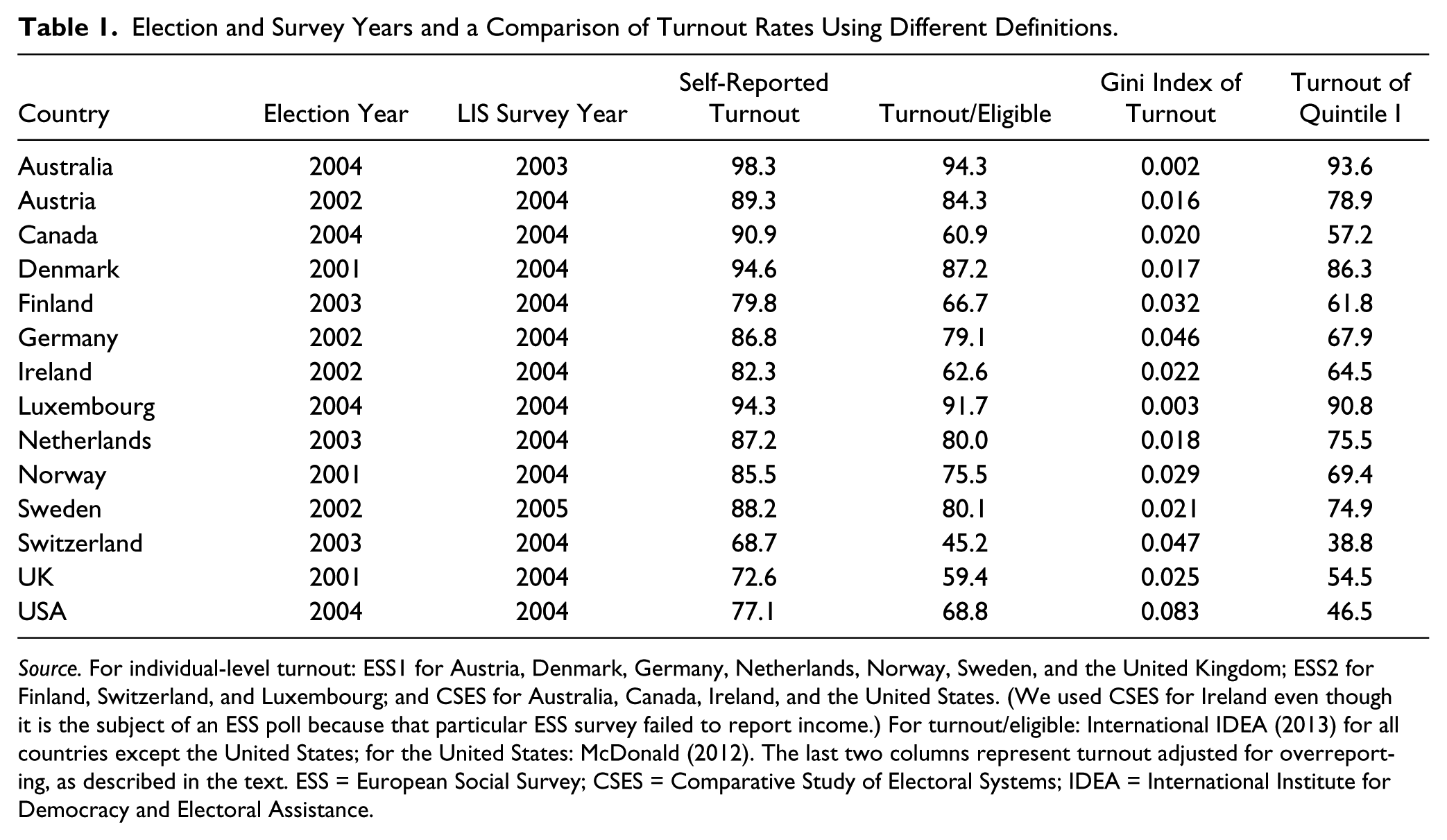
Source. For individual-level turnout: ESS1 for Austria, Denmark, Germany, Netherlands, Norway, Sweden, and the United Kingdom; ESS2 for Finland, Switzerland, and Luxembourg; and CSES for Australia, Canada, Ireland, and the United States. (We used CSES for Ireland even though it is the subject of an ESS poll because that particular ESS survey failed to report income.) For turnout/eligible: International IDEA (2013) for all countries except the United States; for the United States: McDonald (2012). The last two columns represent turnout adjusted for overreporting, as described in the text. ESS = European Social Survey; CSES = Comparative Study of Electoral Systems; IDEA = International Institute for Democracy and Electoral Assistance.

A limitation of a summary measure such as the Gini index is that it represents relative turnout, that is, the variation in turnout across income groups within a given country. A complementary measure can be constructed that focuses on absolute turnout, thus reflecting cross-country rather than intra-country variation. Of special interest is the lowest income quintile. As can be seen in the last column of Table 1, by far the lowest turnout values for the bottom income quintile are found in Switzerland and the United States, where fewer than half of the eligible low-income voters participate. Almost as low are the United Kingdom and Canada, despite their middle-of-the-pack status on the Gini index: in these countries, income groups turn out at fairly similar levels, but turnout across the board is low in comparison to many other countries. At the other end of the scale, turnout for the lowest income group is very high in Australia and Luxembourg, and not much lower in Denmark. In other high-turnout countries, including Austria, the Netherlands, and Sweden, approximately three quarters of the lowest income quintile votes, fairly high by comparative standards, while in Norway, Finland, Germany, and Ireland, the number is about two-thirds.

In concluding this section, we will return to the question posed at the beginning: how well does average electoral turnout, which is the variable employed in almost all previous scholarly work on this topic, serve as a proxy for the income skew of turnout? The relationship is depicted in Figure 1, which relates average turnout on the horizontal axis to the Gini index of the income skew of turnout on the vertical. As can be seen, when average turnout is very high, there is little room for it to vary by income group; this is the case for such high-turnout countries such as Australia, Luxembourg, Denmark, and Austria. As average turnout declines, however, cross-country variation in the degree to which turnout is skewed by income increases. In the middle range of countries, for example, the income skew of turnout is a good deal greater in Germany than its relatively high average turnout would suggest, while the skew in Canada, the United Kingdom, and Ireland is somewhat lower than predicted. At the lowest level of average turnout, represented by the United States and Switzerland, the variation in the degree of income skew is quite wide. Switzerland, despite the lowest average electoral turnout of any country, has an income skew not very different from that of countries with much higher average turnout, notably Germany. The United States, on the other hand, is characterized by an income skew far higher than one would predict from its average turnout, which, while low, is not much different from the average turnout in several other countries with much less income skew. In sum, while it is not unreasonable to use average turnout as a proxy for the income skew of turnout in the absence of more precise data, it is clearly an imperfect proxy. This leads us to ask whether the much-observed relationship between average turnout and government redistribution by way of social transfers continues to hold when a more precise measure is used—which is the topic of the next two sections of the article.

OPEN IN VIEWER

Figure 1.

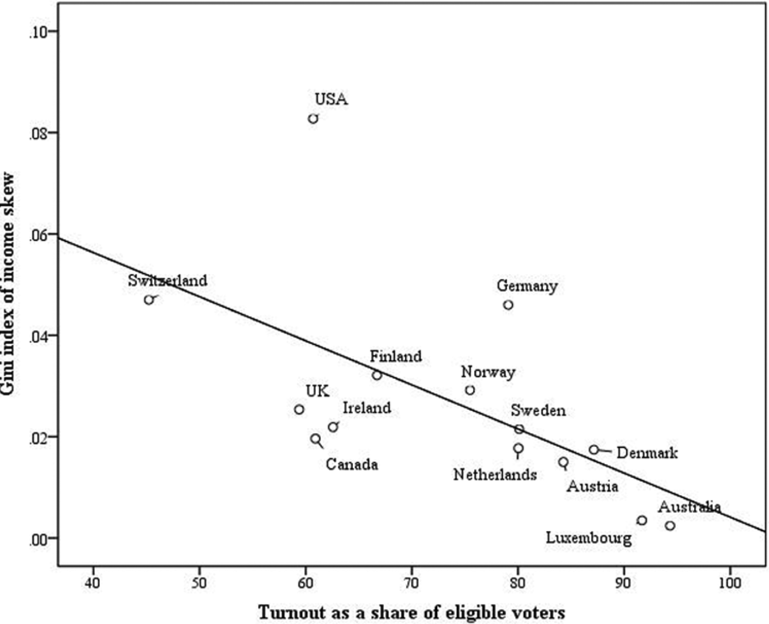
Average Adjusted Turnout Versus Income Skew of Turnout.

Electoral Participation and Government Redistribution: Country-level Analysis

Now that we have developed several measures of the income skew of electoral turnout, we move to our final question: do countries in which income groups vote at similar levels pursue more redistributive policies than those in which a large share of the low-income eligible electorate does not vote? In exploring this question, which reflects a core concern of democratic accountability, we will pursue two empirical investigations. First, we will conduct a country-level analysis in which the income skew of turnout is related to the extent of income redistribution accomplished by social benefit programs, as calculated from the Luxembourg Income Study (LIS). ⁷ Second, we will conduct a multilevel analysis in which data on electoral turnout by income quintile from the ESS or CSES are merged into LIS micro-datasets in an effort to explain variation in the redistributive effect of public benefits, controlling for several household-level demographic and economic variables.

The first question is whether the Gini index of the income skew of electoral turnout helps to explain the degree to which government transfers reduce pre-government income inequality. In using LIS surveys, we have sought to maximize cross-national comparability, even at the cost of reducing somewhat the number of countries compared. Most important, we have focused on redistribution only by way of transfers rather than by way of taxes. The reason for this is that the household-level income surveys on which the LIS relies account primarily for direct taxes such as income taxes and social security contributions; they very rarely account for indirect taxes such as sales, excise, and value-added taxes, which tend to be more regressive than income taxes. From the standpoint of maximizing cross-national comparability, the problem with this is that the share of revenue raised from indirect taxes varies by a factor of more than two to one across the rich OECD countries (OECD 2013), with the result that, if only direct taxes were included, a much smaller share of all taxes paid would be represented in some countries than in others.

With this background, two separate measures of inequality reduction are employed. The first taps the extent to which social benefits reduce overall pre-transfer inequality, measuring the reduction in the Gini index before and after public sector transfers are added to pre-government income. The second focuses on the lowest income group, those in poverty. Specifically, our poverty reduction measure compares pre- and post-transfer values on a composite measure that taps two dimensions of poverty: the share of all households whose income places them below 50 percent of the median income in a given country (the poverty “headcount”) and the difference between the median income of the entire population and the mean income of the poor (defined as above), standardizing by the population median. Multiplying these two measures to form a single indicator, as proposed by Brady (2009), permits us to create a composite indicator of poverty that taps not only how many households are poor but also the depth of their poverty.

Figure 2 depicts the overall relationship between redistribution and the first of these pairs of variables graphically, with redistribution on the vertical axis and the income skew of turnout on the horizontal. As can be seen, the general trend is negative: as the income skew of turnout rises, the extent of government redistribution declines, although the relationship is statistically significant at only the p = .128 level. (Recall that country-level analyses are based on only fourteen cases.) This is, in fact, stronger than the relationship between average turnout and transfer redistribution for these fourteen countries (b = .001 [.001]; t = 1.273 [p = .227], R² = .046), suggesting that using a more precise measure of turnout skew does indeed improve explanatory power.

OPEN IN VIEWER

Figure 2.

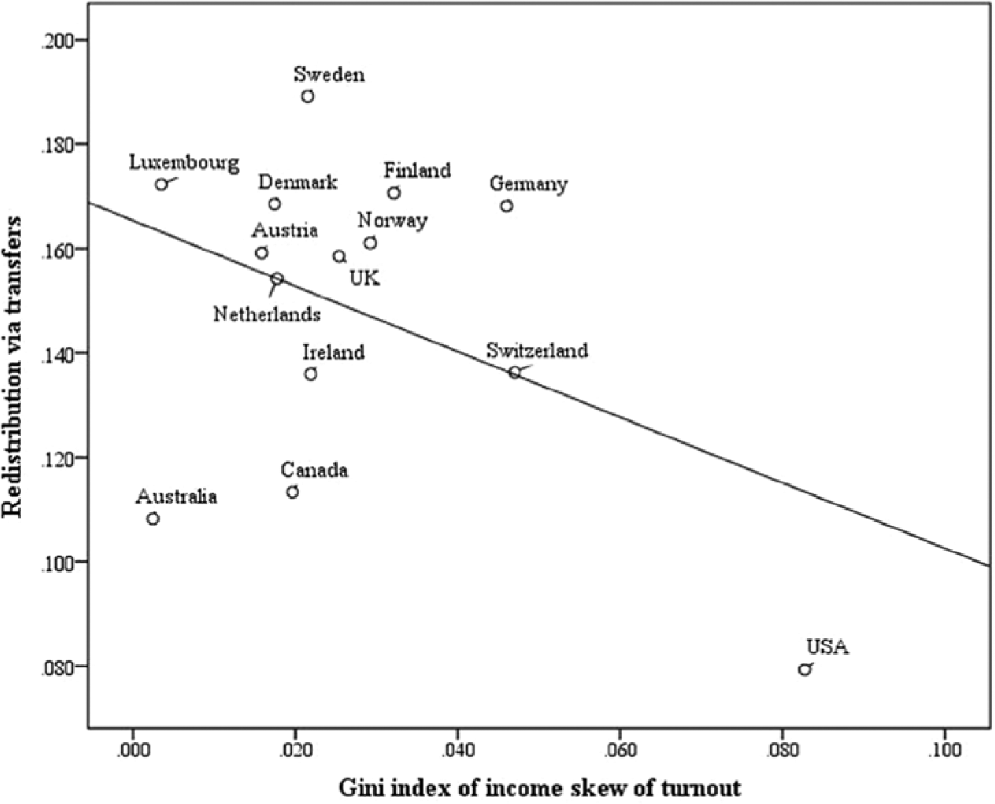
Income Skew of Turnout and Redistribution Via Transfers.

However, as can also be seen, the negative relationship is largely driven by a single country, the United States, whose turnout skew is much higher, and whose transfer redistribution much lower, than those of any other country. There are several other distinctive cases. One is Canada, whose turnout skew is moderate compared with other countries, but which is near the bottom in terms of government redistribution. Similarly, Australia, despite almost no income skew in electoral turnout, is well below average in transfer redistribution. In sum, while there does indeed appear to be a relationship between turnout skew and transfer redistribution, the relationship is not as straightforward as we might expect. In particular, the three non-European countries in our dataset, Australia, Canada, and the United States, vary greatly in turnout skew, but are nonetheless at the low end in terms of transfer redistribution.

A was indicated, the Gini index of the income skew of turnout takes into account only intra-country variation in electoral participation, not variation in absolute turnout across countries. Figure 3 focuses on variation in the electoral participation of the lowest income quintile, measuring how turnout of this quintile in a given country compares to turnout in other countries. Since this analysis focuses on the lowest income group, we have related turnout not to overall government redistribution but rather to the reduction Brady’s poverty measure as a result of public sector social transfers.

OPEN IN VIEWER

Figure 3.

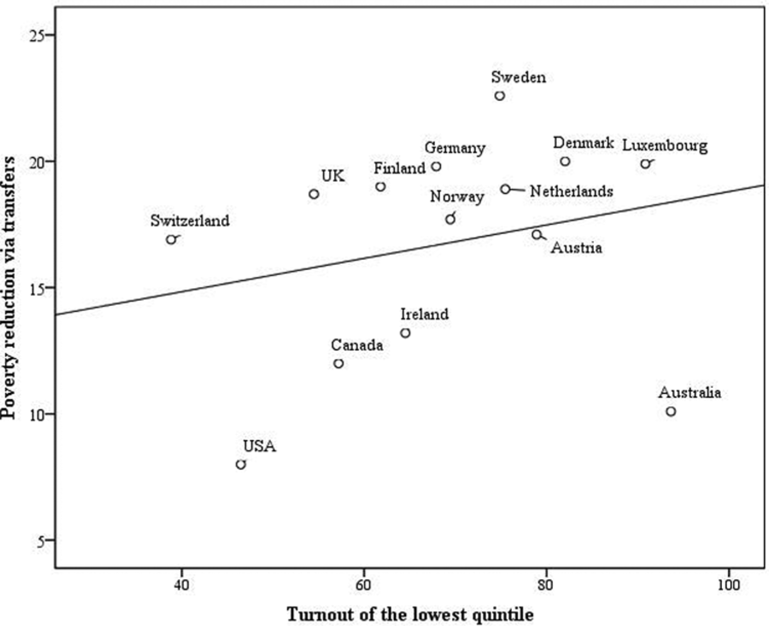
Turnout of Lowest Quintile and Poverty Reduction Via Transfers.

As can be seen, there is a modest positive, but nonsignificant, relationship between electoral participation by this group and poverty reduction as a result of transfer redistribution. Again, there are some deviations for individual countries. In particular, Australia accomplishes a good deal less poverty reduction than the high turnout among low-income groups in that country would suggest. Indeed, if the Australian case is removed, the relationship becomes statistically significant at p = .042 level, even given the small number of cases. Interestingly, poverty reduction by the state is even less in the United States than the very low turnout among low-income groups would lead one to expect. On the other hand, Germany, the United Kingdom, Finland, and Norway, with only middling levels of turnout among the lowest income group, accomplish above-average levels of poverty reduction.

Our analysis is limited by the fact that, with only fourteen cases, degrees-of-freedom problems place severe restrictions on developing a fully specified country-level multivariate model of the sort common in the literature. Still, it is possible to briefly consider a few much-studied variables that have been used to explain cross-country variation in transfer redistribution in the developed world—with the understanding that these variables have been extensively described, measured, justified, and analyzed elsewhere, while the income skew of turnout, the focus of this article, has attracted much less attention. (For a review of this large literature, see Mahler 2010.)

Perhaps the most basic explanatory tradition is the median voter approach, which essentially argues that the more inegalitarian a country’s pre-government income, the more political pressure there will be to redistribute for the simple reason that more voters will gain from redistribution (Meltzer and Richard 1981; Scervini 2012). Another much-examined tradition is the power resources approach, which emphasizes the importance of working-class mobilization, especially by way of leftist political parties (Bradley et al. 2003; Korpi and Palme 2003). A third broad approach focuses on the nature of a country’s electoral system, particularly the claim that proportional representation electoral systems tend to produce more government redistribution than majoritarian systems (Iversen and Soskice 2006).

In considering these relationships, we have constructed multiple regressions that include both our turnout variables and variables associated with the approaches described above. Specifically, in explaining variation in overall transfer redistribution, we have focused on the income skew of electoral turnout and three additional variables: the pre-government Gini index, addressing the median voter approach (calculated from LIS micro-data); a measure from Armingeon et al. (2012) that taps the partisan balance in national cabinets, using a scale that ranges from 5 (“hegemony of social democratic and other left parties”) to 1 (“hegemony of right wing (and centre) groups”); and the Gallagher disproportionality index, which measures the extent to which political parties’ share of the vote in national elections translates into seats in the national legislature, which is, of course, much closer in proportional representation than in majoritarian systems. In explaining variation in poverty reduction, we have included the Armingeon and Gallagher measures as well as a measure of pre-government poverty and turnout in the lowest income quintile.

The results of these regressions are reported in Table 2. As can be seen, the regressions explaining transfer redistribution show that the Gini skew of electoral turnout continues to be negatively related to the extent of transfer redistribution, while the cabinet partisan balance and pre-government Gini are positively related and the Gallagher index negatively related. These results offer some confirmation of the median voter, power resources, and electoral institutions approaches. As to poverty reduction, the results are similar to those in the bivariate case: the turnout of the lowest income quintile is positively, but not statistically significantly, related to government poverty reduction, controlling for other major variables, but the relationship becomes statistically significant when one introduces a dummy variable for Australia.

OPEN IN VIEWER

Table 2.

National-level Regressions on the Reduction in the Gini and Poverty Via Transfers.

	y = Transfer Redistribution	y = Poverty Reduction
	1	1	2
Gini index of turnout skew	−0.893*** (0.220)
Turnout of bottom quintile (Quintile 1)		0.075 (0.058)	0.150** (0.057)
Gini index of pre-government income	0.235*** (0.265)	2.728 (53.918)	−20.311 (44.420)
Cabinet balance	0.012*** (0.004)	1.822** (0.713)	1.667** (0.583)
Electoral disproportionality	−0.004*** (0.001)	−0.384* (0.197)	−0.160 (0.186)
Australia dummy			−8.604** (3.630)
Intercept	0.059 (0.114)	8.263 (23.248)	13.357 (19.022)
R 2	0.724	0.426	0.620

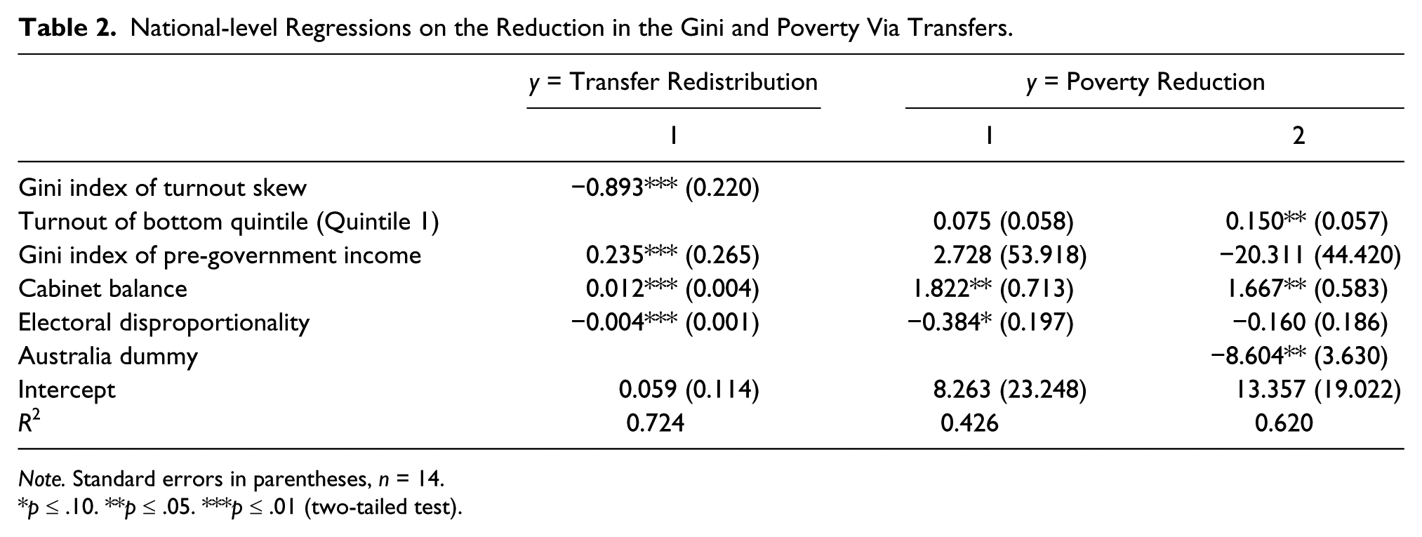
Note. Standard errors in parentheses, n = 14.

*

p ≤ .10. **p ≤ .05. ***p ≤ .01 (two-tailed test).

One would not wish to make too much of these regressions, which are based on a very small number of cases. Still, the fact that our turnout variables continue to be related to government inequality and poverty reduction, even when one controls several other much-examined explanatory variables, increases our confidence that our country-level analysis, if necessarily simple, is not misspecified.

Electoral Participation and Government Redistribution: A Multilevel Analysis

Now that our country-level results have been reported, it is time to move on to a multilevel analysis that includes variables at the level of both individual households and income quintiles. The major advantage of a multilevel analysis of this sort is that it permits us to assess the effect of political participation by various income groups controlling for some of the major household-level characteristics that drive public social benefits in the developed world—characteristics which are largely beyond the ability of political actors to manipulate. Specifically, we have merged quintile-level data on turnout from the ESS or CSES into LIS income surveys, adjusting for overreporting as described earlier.

Our dependent variable is the share of a household’s total income that is supplied by public sector transfers, most commonly in the form of unemployment compensation or old-age pensions; it ranges from 0 to 100 percent. As for the independent variables, there are four. Two are measured at the level of households. The first of these is coded 1 for households that include no earners and no elderly persons, which would make them likely candidates to receive social benefits aimed at the working-age population (particularly unemployment compensation and means-tested public assistance benefits), and 0 otherwise. The second is coded 1 for households that include one or more members aged sixty-five or older, which would make them likely candidates to receive public pensions. Third, of course, we include the average turnout of the income quintile within which each household is located, as described earlier. If electoral participation has an effect on social benefit provision above and beyond the demographic baseline represented by the two household-level variables, we will be able to move beyond our earlier country-level results.

In constructing our multilevel model, we have included one additional second-level variable: a measure of the share of all voters in a given quintile group who indicate in ESS and CSES surveys that they voted for a leftist political party in the election in question. A focus on electoral partisanship is useful for the practical reason that, unlike a number of country-level variables, it can be measured at the quintile level. More generally, a focus on party ideology speaks to the claim of the power resources approach that partisan politics is a critical determinant of public sector transfer redistribution (Korpi and Palme 2003; Bradley et al. 2003). The party classification we have employed is that of Armingeon et al.’s (2012) Comparative Political Data Set I, 1960–2010, which has been widely used in the literature in this area. ⁸ Quintile-by-quintile values are reported in Table A1 of the Online Appendix.

Our basic approach is to conduct five separate multilevel analyses, one for each income quintile, after having merged the LIS income surveys of the fourteen countries we are examining. As has been indicated, the first-level variables are the measures of household-level characteristics that capture the relative “need” for benefits by households, while the second-level variables compare electoral turnout and party support by income quintile across countries. In conducting our multilevel analysis, we have employed the survey weights available in most LIS income surveys, which adjust for under- or over-sampling of certain types of households; quintiles are thus demarcated on the basis of weighted rather than unweighted numbers of cases. As to merging LIS surveys for various countries, the weights of national surveys with different numbers of respondents are adjusted so that they contribute equally to the multilevel analysis. Technical details on the multilevel analysis are provided in the Online Appendix.

The results are reported in Table 3. To start, it is clear that the variables intended to tap households’ “need” for social benefits—and thus their eligibility for social entitlements—are, for every quintile, strongly positively associated with the share of their income that is supplied by the state in the form of social benefits. However, it is of interest that the relationship between these demographic factors and the prominence of public sector transfers becomes somewhat weaker at the top of the income scale. This is hardly surprising: the prominence of social benefits in overall household income would be expected to decrease for the highest-income groups, which have the greatest access to other resources. Still, even for the highest income quintile, the relationship between these demographic variables and social benefit provision remains positive.

OPEN IN VIEWER

Table 3.

Multilevel Results for Share of State Transfers in a Household’s Income: Fourteen Countries.

	Quintile I	Quintile II	Quintile III	Quintile IV	Quintile V
No earners	57.325** (1.763)	70.984** (2.172)	72.427** (3.812)	68.565** (4.819)	53.469** (8.091)
Elderly	60.235** (2.453)	65.132** (1.883)	59.352** (2.802)	50.229** (3.328)	37.914** (3.229)
Adjusted turnout	0.186 (0.121)	0.241* (0.099)	0.196* (0.098)	0.179** (0.068)	0.123* (0.060)
Left party share	0.153 (0.144)	0.042 (0.123)	0.061 (0.094)	−0.006 (0.081)	0.044 (0.079)
Intercept	12.756 (8.877)	−1.118 (8.542)	−4.873 (6.865)	−4.831 (5.836)	−5.439 (4.919)
Intercept variance (Level 2)	33.369 (9.319)	28.201 (9.510)	20.893 (11.948)	14.823 (9.688)	10.320 (5.676)
Residual variance (Level 1)	523.160 (25.687)	434.903 (33.187)	372.596 (25.895)	297.754 (26.368)	202.962 (32.152)
Proportional reduction of variance (Level 2)	0.667	0.825	0.734	0.741	0.751
Proportional reduction of variance (Level 1)	0.605	0.699	0.640	0.556	0.455
R 2	.609	.711	.647	.571	.484

Standard errors in parentheses, n = 289,425 (unweighted total).

*

p ≤ .05. **p ≤ .01 (two-tailed test).

Our main interest in this article is, of course, whether electoral turnout is positively associated with public sector redistribution by way of transfers. For each of our five quintiles, there is indeed a positive slope coefficient relating the turnout of the income group within which a household resides and the share of its income supplied by public social benefits. For example, for the second lowest income quintile, a 1 percent increase in electoral turnout is, on average, associated with a 0.241 percent increase in a household’s receipt of social benefits as a share of its total income above and beyond what one would expect from its objective circumstances. Thus, a 25 percent increase in the turnout rate of households in this quintile (approximately the difference between Germany and the United States) is, on average, associated with a 6 percent increase in the share of social transfers in total income, after accounting for demographic factors. The slope coefficient declines to 0.196 for the third quintile, to 0.179 for the fourth, and to 0.123 for the highest. Only for the lowest income quintile does the relationship fail to achieve statistical significance, although even here the relationship is positive.

As to our left party variable, there is less to say. In short, the support among income quintile groups for socialist and other leftist political parties is not significantly related in either direction to the prominence of social transfers for any quintile, controlling for the turnout of that group, although the relationship is stronger for the lowest income quintile than for the others and is in all but one case positive. Although we would certainly not wish to push this point too far, given that we are examining only fourteen cases, it appears that the partisan orientation of the party for which an income group votes may be less important than whether it votes in the first place.

Measures of the overall fit of the models are reported in the last three rows of Table 3. It is noteworthy that a substantial share of the total variation in state redistribution is explained by cross-national variation in electoral turnout. As can be seen, the proportional reduction in variance at the country level (Level 2) is greater than the proportional reduction of variance at the individual level (Level 1) in each of the quintiles. The adjusted R-squared, which summarizes the goodness of fit of the model as a whole, ranges from 0.711 in the second quintile to 0.484 in the fifth.

In sum, we find support in the multilevel analysis for our expectation that electoral participation matters. Specifically, higher electoral participation by income groups, especially those in the lower-middle and middle parts of the income spectrum, is indeed associated with greater redistribution in their favor. Certainly, the baseline of “need” determines the basic structure of benefit provision. Still, electoral participation does appear to explain a substantial share of cross-national variation in transfer redistribution above and beyond this baseline.

Conclusion

The overall goal of this article has been to explore the relationship between the income skew of electoral turnout in the developed world and the degree of income redistribution accomplished by social transfers. One of our intended specific contributions has been in the area of measurement; in particular, we have moved beyond the usual strategy of employing average turnout in a country as an imperfect proxy for the income skew of turnout. In offering a more precise measure, we have also addressed a number of longstanding measurement issues in this area, notably the overreporting of turnout in individual-level election studies.

A second contribution has been to offer a preliminary analysis of the relationship between several aspects of the income skew of electoral turnout and the extent to which the state redistributes market income. We began with a country-level analysis focusing on variation in individual income quintiles’ turnout, both within and across countries. This was followed by a multilevel analysis in which turnout levels by quintile were merged into income surveys from the Luxembourg Income Study, in an effort to explore whether electoral participation explains variation in transfer redistribution above and beyond the effect of household-level variables associated with programs aimed at the working-age and elderly populations.

Our overall conclusion is that turnout is indeed positively associated with transfer redistribution, although many other variables also play a role. The fact that this hypothesized relationship has withstood a more rigorous empirical test than has commonly been the case increases our confidence that it is indeed in evidence. In sum, we believe that the analysis reported here has made a tangible contribution not only to the measurement of electoral participation but also to our understanding of its policy consequences.

Beyond this, our contribution has implications for broader concerns about democratic accountability at a time of increasing income inequality throughout the developed world. These implications are particularly pertinent in light of concern (e.g., Schlozman, Verba, and Brady 2012; Stiglitz 2012, 135–38) about growing inequality of inputs into politics that, it is widely believed, has increasingly constrained traditional government efforts to ameliorate income inequality generated by the market.