What Are Friends for? The Effect of Geographic Proximity on Primary Turnout in Gubernatorial Elections

Abstract

“Friends and neighbors” voting is the tendency of candidates to earn a higher than expected share of the vote in their home counties and states. This hometown effect has been witnessed across an array of elected offices and time periods, prompting researchers to examine how local candidates impact voters’ turnout decisions and electoral choices. This paper focuses on the effect of hometown candidates on turnout using voter rolls and histories from Ohio and Georgia during the 2018 gubernatorial primary elections. These administrative data allow us to observe the decisions of all registered voters in both of these contests along with, importantly, their prior turnout history. We find a consistent relationship between the presence of a hometown candidate and turnout decisions; however, this effect is conditional on voters’ previous vote histories in primaries. The effect is strongest among those who occasionally vote in elections, smaller for those who habitually vote, and negligible for those who have never participated before. These results contribute to our understanding of how the presence of local candidates translates into support for their campaigns, and provide evidence that the size of this effect is not the same for all voters.

Keywords

gubernatorial elections voter turnout political geography primary elections

Voter turnout is one of the most important and fundamental aspects of a functioning democracy. Concerns over low turnout constantly loom over elections in the United States, especially in nonpresidential election years and in primary elections. As such, there is a large body of literature examining voter turnout, and we know much about factors that impede or increase the likelihood of voting at both individual and aggregate levels. However, much of this research examines both general elections and federal elections. Overall, we know less about the decision to vote in primary elections, especially state-level primary elections. In this paper, we examine the potential for local¹ candidates to mobilize turnout in gubernatorial primaries, conditional on an individual’s previous participation in primary elections.

Candidates running for office tend to receive higher vote shares in their home counties and states. This electoral phenomenon, illustrated most famously in Key’s (1949) examination of political behavior in the American South, is documented across several time periods and electoral contexts.² Local candidates receive more support from their “friends and neighbors,” those voters who live within the candidate’s county or state of residence. Explaining the causal process through which geographic proximity is translated into support for the so-called hometown candidates is the subject of recent scholarship. Some contend that voters put aside other allegiances to support local candidates (Kawai and Watanabe 2013), while others suggest that hometown candidates increase the likelihood people turn out to vote in the election (Bhatti and Hansen 2016). This paper contributes to this latter explanation, demonstrating that candidates draw increased numbers of local voters to the poll and that some potential voters are more likely to turn out than others.

This study builds on previous scholarship in two principle ways. First, we use novel data: the voter rolls and histories of Georgia and Ohio during the 2018 gubernatorial elections. These administrative data allow us to examine every registered voter in a state, their history of participating in elections, and their decision to turn out in 2018. In addition, having access to voter addresses allows us to determine if the individual voter lives in the county or media market of a candidate, as well as their geographic distance to those running. These data allow us to build on previous studies that rely on aggregate city or county statistics to explore the microlevel decisions of individual voters. Second, voter history data enable us to differentiate between those voters with a higher predisposition to participate in elections versus others. We can avoid concerns about the social desirability bias inherent in asking voters if they participated in survey questionnaires, and are able to observe these patterns directly using administrative data (Brenner and DeLamater 2016; Cooper, Knotts, and Haspel 2009). We find that the hometown effect is strongest for voters who occasionally participate in primary elections, negligible for those who have never participated, and small for those who habitually turn out. Before turning to these data, however, we first trace the development of the “friends and neighbors” literature, discuss the importance of the predisposition to turnout as it relates to our argument, and outline our expectations.

What Is Friends and Neighbors Voting?

Friends and neighbors voting is a term used to describe the reality that “candidates for state office tend to poll overwhelming majorities in their home counties and to draw heavy support in adjacent counties” (Key 1949, 37). Key (1949) identifies support for the hometown candidate in a variety of southern states. In these states, with multiple competing sources of power within the Democratic Party, allegiance to the local candidate is found to play a powerful role in voters’ electoral calculations. Subsequent scholarship documents the impact of geographic proximity in a variety of contexts and time periods. For example, friends and neighbors voting is found to impact elections to statewide offices in Mississippi from 1943 to 1973 (Tatalovich 1975), in the election of George Wallace as governor of Alabama (Black and Black 1973), and in several other gubernatorial, primary, special, and judicial retention special elections (Aspin and Hall 1989; Van Wingen 1984; Van Wingen and Parker 1979). Even presidential candidates have been found to perform well in their home states, receiving a higher share than comparable nonlocal copartisans (Dudley and Rapoport 1989; Garand 1988; Lewis-Beck and Rice 1983).

The size of the hometown effect, while often modest in absolute terms, can be large enough to potentially influence close elections. In Key’s (1949, 39) one-party South, assembling a local base of electoral support was often necessary to securing election:

In a sense the battle of state politics is not a battle between large party factions. It is rather a struggle of individuals—perhaps with the support of their county organizations—to build a state-wide following on the foundation of local support.

The willingness of voters to support their local candidate, however, may have been the product of their rational desires to have local interests advanced in state government, or the feeling of loyalty they may have felt to members of their community, especially in one-party environments. This feeling of loyalty appeared to be larger in smaller, rural areas compared with larger cities (Key 1949, 40–41). However, in the absence of any party cue to guide their behavior, these results suggest that voters turn to other heuristics—namely, the presence of a local candidate—to aid in their decision making.

Why and How Are Local Candidates Supported?

Two causal mechanisms are commonly advanced explaining the hometown effect. The first is based on the mobilization of voters, and the second, on the ability of local candidates to persuade (Panagopoulos, Leighley, and Hamel 2017). The mobilization hypothesis supposes that the higher vote shares observed for hometown candidates reflect those, who would have otherwise stayed home, turning out to support their local candidate. Increased support for the candidate is, therefore, the product of higher participation by voters who are pulled into the contest because a hometown candidate is running. Subsequently, we would expect that these same voters are less likely to participate when a local candidate is not present on the ballot. The persuasion hypothesis states that voters, who would otherwise cast their ballots for some other candidate, put these other allegiances aside to support their hometown candidate (Panagopoulos, Leighley, and Hamel 2017). In this case, we expect Republicans to vote for a Democratic candidate if they are local (and the Republican candidate is not) and vice versa.³ Here, we focus on the former explanation—the ability of hometown candidates to compel the participation of voters who may not have otherwise turned out—examining both the characteristics of voters that make them more likely to turn out to support hometown candidates and who they consider to be a local candidate.

It is important to understand who voters consider to be local candidates. In Key’s (1949) study of the phenomena, local candidates are those living in the same county as the voter. In addition to counties sometimes serving as the locus of political power in particular jurisdictions, studies of electoral behavior reveal that gathering information about candidates is costly (Downs 1957) and that voters often rely on heuristics to make electoral decisions (Converse 1962). Most voters, however, do not approach elections as blank slates, but have been educated by previous contests, the information conveyed by candidates and the media over the course of campaigns, and the process of living within a community and being exposed to local politicians (Bowler, Donovan, and Snipp 1993; J. E. Campbell, Alford, and Henry 1984). The importance of counties may reflect—in part—how information is dispersed across geographic space.

Panagopoulos, Leighley, and Hamel (2017) also demonstrate the importance of sharing the same county as a candidate in their turnout experiment. Here, they find a positive relationship between those who are told a candidate lives in the same county and their likelihood of voting in the election. Potential voters who were told they live in the same city as the candidate, however, are no more likely to participate (Panagopoulos, Leighley, and Hamel 2017). These results suggest that even when we examine more recent elections, voters may place more value in sharing a home county (increasing turnout by 5.8% in their study) compared with the same city (Panagopoulos, Leighley, and Hamel 2017).

The impact of sharing a home county with a candidate is also demonstrated when examining electoral results. Gimpel et al. (2008) explore the effect of geographic distance on the electoral support received by gubernatorial candidates by measuring the distance between the candidate’s home county and all other counties in the state. They conclude that distance does not have a linear effect on support, but that its effect decays after some critical distance from the candidate’s home county is crossed (Gimpel et al. 2008). Their research also reveals that it is important to consider not just the proximity of a county to a candidate, but also its distance from the opposing party’s nominee (Gimpel et al. 2008).

Friends and neighbors voting, therefore, drives higher vote shares for candidates in their home counties. Still, its effect may be nuanced, depending, for example, on the presence of other candidates from the same geographic area, the type of race run, and the presence of other, more salient, turnout considerations. In addition, these studies demonstrate that who voters consider to be hometown candidates may also vary. Living in the same county as the candidate appears to be salient across a variety of contexts (when examining races for state offices), and states matter when considering support for presidential nominees.

Prior Voting History

Not all individuals are equally likely to turn out in any given election, and this is an important component when examining any campaign or get-out-the-vote (GOTV) effort. While there is extensive literature on the factors that influence turnout, one generally consistent finding is that previous turnout influences the likelihood of future voting (Gerber, Green, and Shachar 2003; Green and Shachar 2000). However, as Arceneaux and Nickerson (2009) discuss, there is less consensus on the conditional role of voter propensity in specific electoral or campaign contexts and turnout in a given election. They find, in terms of GOTV efforts, that “canvassing increases turnout mostly by enticing those who are on the cusp of voting” (Arceneaux and Nickerson 2009, 12). This fits with Niven’s (2001, 2004) argument of a curvilinear relationship between campaign messages and turnout; habitual voters do not need an additional incentive or cue to vote, while those disengaged from politics are unlikely to remember (or care about) campaign messages. Essentially, habitual voters are often immune from campaign or GOTV appeals as they are most likely going to vote anyway (Denny and Doyle 2009; Plutzer 2002). On the other end of the spectrum, nonvoters are likely to stay nonvoters (Fowler 2006; Kahn and Kenney 1999). It is those voters in between these two spectrums that appear ripe for campaign, contextual, or GOTV efforts to have an influence on their turnout decisions.

Expectations

In this paper, we examine the presence of a local candidate on the probability that a voter participates in a primary election. Primaries for state office provide a unique opportunity to examine the effect of geographic distance at an individual level. Studies of American voters have long revealed that many voters lack detailed information about the various candidates running and their issue positions. Instead, these voters are thought to rely upon heuristics to guide their voting decisions (A. Campbell et al. 1960; Popkin 1991). Primaries often attract less media attention than general elections, and voters are forced to make decisions without access to the one heuristic consistently demonstrated to have a large impact on their choices: partisanship. The presence of a local candidate can fill this void, providing local voters with information about the candidate that nonlocal voters may lack. By providing voters with the opportunity to support (or oppose) a “home team” candidate, local voters may now have an incentive to participate in the primary election.⁴ Similarly, the presence of a local candidate may generate more local media attention and “buzz” about the upcoming election. This, in turn, may serve to stimulate local voter turnout.

In primary elections, one cue voters can use in deciding how to cast their vote is their ability to assess if a particular candidate is like themselves (Cutler 2002; Fenno 1978; Popkin 1991). The hometown of the candidates running provides information that may be relevant to some subset of voters. Name recognition also plays a large role in low-information contests, and both money and prior experience running and holding office are two keys to achieving success in primary races (Morehouse 1990; Stone and Maisel 2003; Taebel 1975). While Key’s (1949) theory is principally based on the proclivity of local voters to support local interests, building from the mobilization hypothesis from Panagopoulos, Leighley, and Hamel (2017), we argue that the friends and neighbors effect is especially relevant for driving turnout in primaries. The presence of a local candidate can lead to more available information or awareness about the upcoming election for potential voters. This can happen in several ways, including additional local media coverage of the candidate and the election. Candidates may be better able to spread their message to those more geographically proximate to their homes and be able to better identify with these local constituencies; these actions could increase name recognition and serve as a cue to spur turnout in the election.

Similar to the effects of GOTV mobilization drives, we do not expect this hometown effect to apply equally to all registered voters (Arceneaux and Nickerson 2009; Enos, Fowler, and Vavreck 2014). The potential informational advantages of having a local candidate are not going to have the same influence on everyone; therefore, we distinguish between those voters who always participate in elections, those that occasionally participate, and those who have never participated. We expect the effect to be strongest for occasional voters, those individuals with a voting history of turning out in some, but not all, primary elections. For individuals with no primary voting history, this informational cue of a hometown candidate could be enough to get them to vote, but we think that is giving the influence of a hometown cue perhaps too much credit, and they will remain unlikely to turn out. For those individuals who always vote in primaries, while they may be aware of the local candidate, their likelihood of turning out was already high and the effect of a local candidate may be moot.

Case Selection

Our focus is on the potential for a friends and neighbors effect for top of the ballot statewide elections. “Down ticket” races, such as those for state assembly and State Senate seats, receive far less attention than high-profile, statewide races such as gubernatorial contests. They would, thus, present a wholly different electoral environment than the one we are exploring (Garlick 2015). In addition, we want to focus on the impact of statewide elections, so we examine turnout in the 2018 elections to avoid the confounding issue of having the presidential race on the ballot. Given the incumbency advantage and often lack of competitiveness in gubernatorial primaries with an incumbent running (Bardwell 2002), we limit our potential case selection to states with open-seat gubernatorial elections in 2018. One final aspect we consider in case selection is the primary system used in the states.

States with a closed or partially closed primary⁵ limit the ability to test for a hometown effect since only individuals registered with a party can vote in that party’s primary. While our focus in this paper is not directly on partisan turnout, we wanted an environment where all registered voters were eligible to vote in the primary without partisan limitations. We focus on states with an open or partially open system to draw our cases. Open primaries allow voters to select a party ballot on Election Day and do not require a previous party registration to be eligible to vote in the primary. Six states, Georgia, Michigan, Minnesota, Ohio, Tennessee, and Wyoming, fit these requirements. Finally, given the historical focus on friends and neighbors studies in southern states, we selected one southern state for analysis along with a nonsouthern state for comparison purposes.

From there, we inquired into the availability of both voter registration rolls and voter histories. Ohio’s was free and publicly available from the Secretary of State and Georgia’s voter history files were free and publicly available while we had to purchase the voter registration roll from the Secretary of State’s office. The other four states either had more burdensome requirements for obtaining the data, or it was not obvious that both data components were readily available. Given this and the large size of the data files, our case selection in this paper is Georgia and Ohio.

These states provide some variation between them. Georgia is an open primary state, with no partisan labels attached to a registered voter, whereas Ohio is partially open, which means that registered voters are listed as belonging to a party based on previous primary vote history or by selection at time of registration. However, in Ohio, voters are eligible to select any party ballot regardless of listed party registration on Election Day. In Georgia, we only examine the hometown candidacy for the gubernatorial candidates, as the lieutenant governor is elected separately from the governor. With no U.S. Senate seat on the ballot, governor is the clear top of the ballot race in Georgia during 2018. Ohio is a bit different. First, the presence of a U.S. Senate race means that voter attention may have been split between this race and the gubernatorial contest. Second, Ohio uses a presidential-style joint ticket for governor and lieutenant governor, meaning that the candidates for the two positions in Ohio run on a single ticket. For this analysis, we focus only on the gubernatorial candidate while ignoring the lieutenant governor position. To check the robustness of our results, we also ran a similar analysis examining the U.S. Senate race and find similar hometown effects as those reported for governor.⁶

Data and Method

To test our expectations, we use full voter registration rolls from Georgia and Ohio for the 2018 primaries along with voter history information. Georgia provides separate voter history files for elections back to 1996. We match these files with the current registration rolls. Ohio provides voting history dating back to 2000 included in the voter registration rolls. This provides us with all possible voters to determine who turned out to vote in the primary. We drop voters from both states listed as inactive on the voter roll and those registered after the cutoff date for eligibility to vote in the 2018 primary.

The dependent variable in each model is dichotomous, indicating if the registered voter participated in the primary. To assess the effect of friends and neighbors voting, we begin by creating two categorical measures. The first indicates if the registered voter lives in the same county as a gubernatorial candidate. Next, we expand the analysis of geographic proximity in two ways, measuring if a voter lives in a county adjacent to a gubernatorial candidate and if the registrant shares the same media market as someone running.⁷ This expanded coding allows us to see if there is something unique about living in the same county as the candidate or if the hometown effect translates to a larger geographic area perhaps as a function of voters being more aware of local candidates as media markets can influence turnout and candidate support (Althaus and Trautman 2008; J. E. Campbell, Alford, and Henry 1984). Second, we replace these categorical measures of the hometown effect with the distance (in miles) a registrant lives from the nearest gubernatorial candidate to provide another measure of proximity. For this, we geocode each registered voter’s zip code and the zip code of the home address for each of the gubernatorial candidates.⁸ We then calculate the distance in miles to the nearest gubernatorial candidate on the ballot.⁹

We expect any proximity effect to be moderated by someone’s likelihood of voting in a primary election. To capture this, we determine each registered voter’s previous turnout in primary elections. In both states, only the date an individual registered in their current county is available, and not the date of original registration in the state. Therefore, we create a variable for the percentage of primaries voted in based on all available primaries in the data sample. Given the expected conditional effect of previous voter turnout, the variable of primary interest in each model is the interaction between the geographic proximity variable and previous turnout.

Figure 1 shows the home locations and media markets of the candidates in both states, while Table 1 shows the descriptive statistics for geographic proximity and previous turnout variables. As shown in Figure 1, Georgia has 159 counties or the second most in the nation, while Ohio has eighty-eight counties, also above the national average of sixty-three counties per state. In Georgia, the geographic proximity is fairly evenly distributed across the four categories as 22.14 percent of the state’s registered voters lived in a county that one of the gubernatorial candidates resided, 23.62 percent living in a county adjacent to a candidate’s home county, 24.32 percent lived within the same media market as a candidate (but not in the same or an adjacent county), and 30.01 percent lived outside of these areas, so they did not have a geographically proximate candidate according to our coding scheme. Meanwhile, the average registered voter lived 52.54 miles from the nearest candidate. The registered voters had participated, on average, in 11.94 percent of the state’s previous primary elections in the sample.

Figure 1.

Candidate home counties and media markets.

Table 1.

Descriptive Statistics.

	Georgia	Ohio
Percent with a hometown candidate	22.14	38.95
Percent in adjacent county	23.62	27.46
Percent in media market only	24.23	8.62
Percent with no proximate candidate	30.01	24.97
Mean closeness to candidate (miles)	52.54 (61.76)	31.81 (28.21)
Mean previous primary voting (%)	11.94 (22.51)	24.93 (28.63)

This table reports the percent of registered voters in Georgia and Ohio who live in the same county as a candidate running for governor, live in an adjacent county to a candidate, live in the same media market, or live outside this range. It also presents the average proximity of each voter to their nearest candidate and the percent of voters who participated in the previous primary elections found in the dataset (standard deviations for each mean are reported in parentheses).

In Ohio, 38.95 percent of registered Buckeyes shared a county with a gubernatorial candidate, 27.46 percent lived in an adjacent county, 8.62 percent lived within a candidate’s media market, and 24.97 percent did not have a proximate candidate. The average person lived 31.81 miles away from the nearest gubernatorial candidate and had turned out for 24.93 percent of the state’s previous nine primary elections.

Results

Tables 2 and 3 show the results for 2018 primary turnout in Georgia and Ohio, respectively. Each model is estimated using a logistic regression equation, indicating if the registered voter turned out or not. We include multiple specifications, testing the importance of living in the same county as a candidate, living in a county proximate to a candidate, examining the effect of distance measured continuously, and revisiting the base model controlling for other demographic characteristics available in the voter files.¹⁰

Table 2.

Turnout Model Results: Georgia.

	Model 1: hometown	Model 2: geographic proximity	Model 3: distance	Model 4: hometown with controls
Hometown candidate^a	0.2026* (0.0034)	0.2642* (0.0040)		0.2341* (0.0034)
Candidate in media market^a		0.1996* (0.0043)
Candidate from adjacent county^a		0.0166* (0.0041)
Distance (miles) to the nearest candidate			−0.0016* (0.0000)
%Voted in previous eligible primaries	4.5333* (0.0052)	4.4315* (0.0076)	4.7824* (0.0066)	4.9173* (0.0073)
Interactions
Hometown candidate × %Voted	0.4254* (0.0125)	0.5272* (0.0137)		0.3904* (0.0125)
Media market × %Voted		0.0908* (0.0128)
Adjacent county × %Voted		0.3830* (0.0129)
Closeness × %Voted			−0.0025* (0.0001)
Controls
Age				0.1020* (0.0004)
Age²				−0.0008* (0.0000)
Years registered in county				−0.0257* (0.0001)
African American^b				0.1245* (0.0027)
Other^b				−0.2109* (0.0041)
Female				0.0478* (0.0024)
Constant	−2.2759* (0.0017)	−2.3375* (0.0028)	−2.1462* (0.0019)	−4.8962* (0.0109)
No. of observations	6,064,161	6,064,161	6,060,687	6,055,186

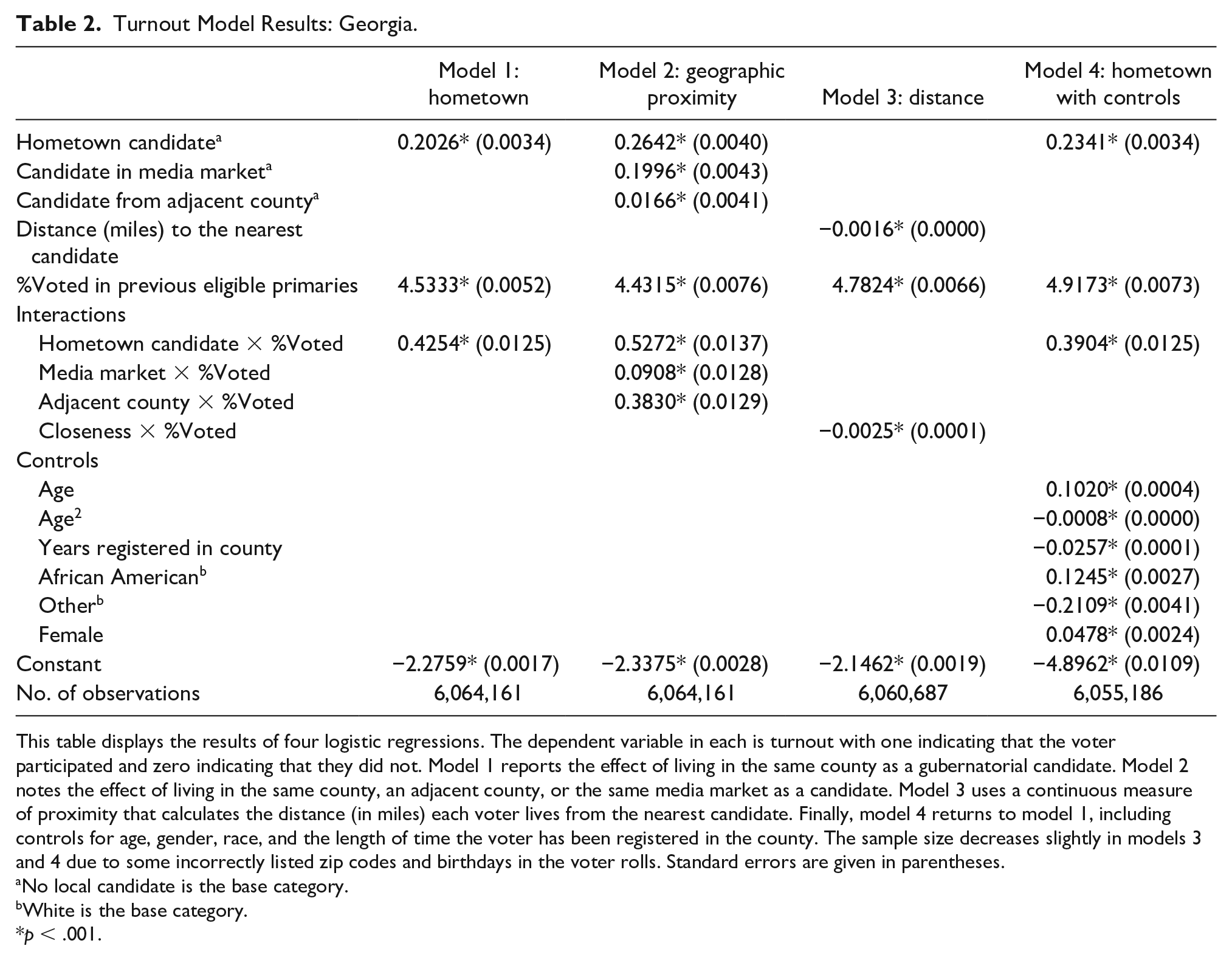
This table displays the results of four logistic regressions. The dependent variable in each is turnout with one indicating that the voter participated and zero indicating that they did not. Model 1 reports the effect of living in the same county as a gubernatorial candidate. Model 2 notes the effect of living in the same county, an adjacent county, or the same media market as a candidate. Model 3 uses a continuous measure of proximity that calculates the distance (in miles) each voter lives from the nearest candidate. Finally, model 4 returns to model 1, including controls for age, gender, race, and the length of time the voter has been registered in the county. The sample size decreases slightly in models 3 and 4 due to some incorrectly listed zip codes and birthdays in the voter rolls. Standard errors are given in parentheses.

No local candidate is the base category.

White is the base category.

p < .001.

Table 3.

Turnout Model Results: Ohio.

	Model 1: hometown	Model 2: geographic proximity	Model 3: distance	Model 4: hometown with controls
Hometown candidate^a	0.0724* (0.0035)	0.1415* (0.0045)		0.0922* (0.0036)
Candidate in media market^a		0.0662* (0.0070)
Candidate from adjacent county^a		0.1321* (0.0049)
Distance (miles) to the nearest candidate			−0.0025* (0.0001)
%Voted in previous primaries	4.5132* (0.0048)	4.6334* (0.0077)	4.6598* (0.0058)	4.355* (0.0054)
Interactions
Hometown candidate × %Voted	0.2487* (0.0080)	0.1285* (0.0100)		0.2691* (0.0081)
Media market × %Voted		−0.0848* (0.0150)
Adjacent county × %Voted		−0.2381* (0.0105)
Closeness × %Voted			−0.0017* (0.0001)
Controls
Age				0.0378* (0.0004)
Age²				−0.0003* (0.0000)
Years registered in county				−0.0016* (0.0000)
Constant	−2.6182* (0.0022)	−2.6873* (0.0036)	−2.5111* (0.0026)	−3.6292* (0.0094)
No. of observations	6,817,139	6,817,139	6,817,139	6,817,139

This table reports the results of four logistic regressions. The dependent variable for each is turnout with one indicating that the voter participated and zero indicating that they did not. Model 1 reports the effect of living in the same county as a gubernatorial candidate. Model 2 notes the effect of living in the same county, an adjacent county, or the same media market as a candidate and model 3 uses a continuous measure of proximity that calculates the distance (in miles) each voter lives from the nearest candidate. Model 4 returns model 1, adding controls for the age of the voter and the years they have been registered to vote in the county. Standard errors are given in parentheses.

No local candidate is the base category.

p < .001.

With more than six million registered voters in each state, it is not surprising that all the variables in each model achieve traditional levels of statistical significance. In each model across both Georgia and Ohio, the coefficients are in the expected direction and indicate that having a hometown candidate or other geographic proximate candidate leads to greater turnout, while living further away from the nearest candidate leads to a decrease in turnout.

To examine the substantive effects in Georgia, Figure 2 provides the predicted probabilities and marginal effects for the likelihood of primary turnout for those voters with a hometown candidate and those without based on model 1 in Table 2. The top figure shows the predicted probabilities across the range of previous turnout by hometown candidate status, while the bottom figure shows the difference in marginal effects between having a hometown candidate and not across previous turnout. Given the dichotomous hometown candidate variable, this is showing the difference between the two predicted probabilities from the top figure. We show the results both ways to highlight the overall likelihood of turning out based on previous voting habits as well as the substantive difference of having a hometown candidate.

Figure 2.

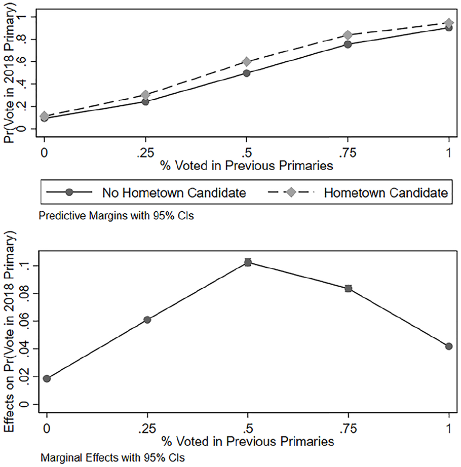
Predicted probabilities and marginal effects for hometown candidate: Georgia.

Starting with nonvoters, or those who had not voted in any previous primary in our sample, we find that they are highly unlikely to vote in 2018, with a 10 percent predicted probability of turning out; however, the nonvoters with a hometown candidate were 2 percentage points more likely to vote (11.2% compared with 9.3%). Moving into the occasional voters, individuals that had voted in 25 percent of the previous primaries had a likelihood of voting in the 2018 primary of 30 percent for those with a hometown candidate and 24 percent for those without a local candidate. People having voted in half of their previously eligible primaries are predicted to turn out between 50 percent (non-hometown candidate) and 60 percent (hometown candidate). Those voting in 75 percent of their previously eligible primaries have a predicted likelihood of turning out at between 75 percent (non-hometown candidate) and 84 percent (hometown candidate). Looking at the habitual voters (voted in 100% of previously eligible primaries), the likelihood of turning out is between 91 and 95 percent. Once again, individuals with a hometown candidate are more likely to turn out than those without one even among those most likely to vote in the first place. However, the difference is only around 5 percent. Focusing on the bottom panel of Figure 2, the largest hometown effect is on those occasional voters with between 50 and 75 percent previous turnout.

In Ohio (Figure 3), the results show a similar pattern but with an attenuated hometown effect. The likelihood of voting based on previous voting history is similar in both states, but the hometown effect is smaller across the range of previous voting history in Ohio compared with Georgia. There is virtually no local candidate bump for those with no previous history (0.47%), while, for those that had voted in 25 percent of the previous primaries, there is a 2.1 percent predicted increase for registered voters living in the same county as a candidate. The strongest effects are once again for those occasional voters in the 50–75 percent previous turnout range. However, unlike Georgia, the hometown effect is largest (5.3%) for those that had voted in 75 percent of the previous primaries with the hometown effect being slightly less (4.8%) for those voting in half of the previous primaries. Finally, for the habitual voters, those with a hometown candidate are predicted to have a 3.2 percent increase in turnout compared with those without a local candidate on the ballot.

Figure 3.

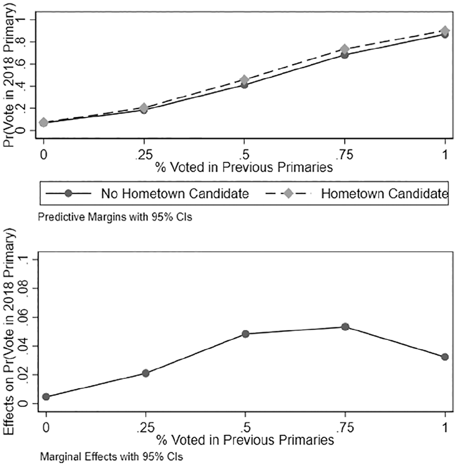
Predicted probabilities and marginal effects for hometown candidate: Ohio.

For traditional nonvoters, occasional voters, and habitual voters, there is a clear pattern of those living in the same county as a gubernatorial candidate having a greater likelihood of turning out. The hometown bump varies as predicted with the smallest effects on nonvoters followed by habitual voters and the strongest effect on occasional voters, especially those who had voted in between 50 and 75 percent of the previous primaries.¹¹

Figure 4 presents a more detailed look at geographic proximity to a candidate by accounting for adjacent counties and those nonadjacent counties that share a media market with the candidate’s home county. Here we show only the marginal effects or the discrete change from the base category of not having a hometown candidate. The results in Georgia (top panel) show similar effects for individuals living in adjacent counties and within the broader media market on their likelihood of turning out. For those living in an adjacent county to a candidate, there is virtually no effect for individuals without a voting history and this increases to a 5.6 percent higher likelihood of turning out for those individuals that had voted in 75 percent of the previous primaries. For those living within the media market, the results are slightly stronger, with the strongest effect being a 6.1 percent predicted increase for those who had voted in half of the previous primaries. The results for those having a candidate from their county follow the same pattern as in Figure 2, but the effect is slightly stronger across the range of voting histories. This makes sense as the change in the variable coding only shifted registered voters out of the non-hometown candidate category.

Figure 4.

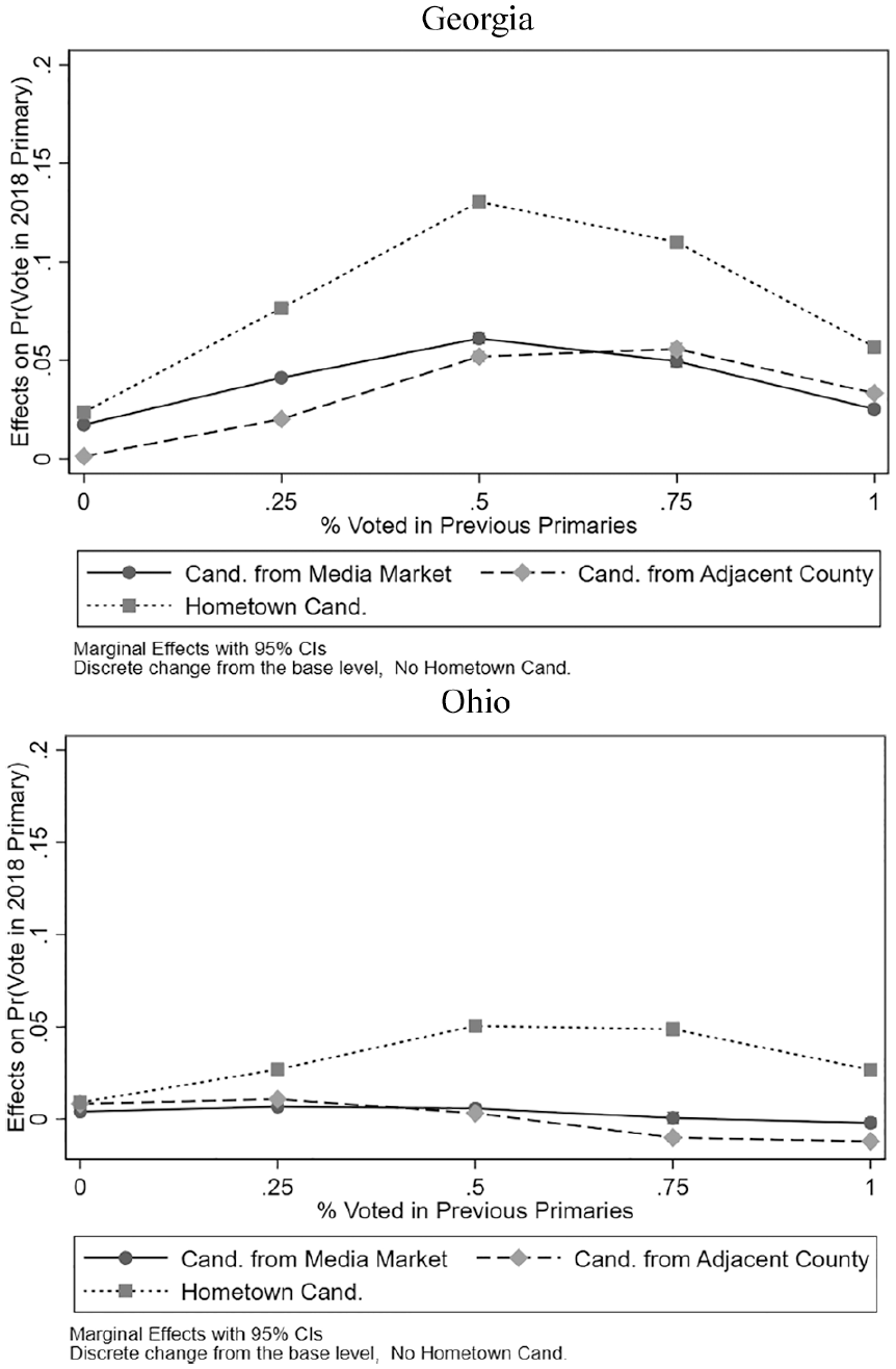
Marginal effects for geographic proximity model: Georgia and Ohio.

The bottom panel shows a slightly different pattern for Ohio. Here there is no substantive difference between not having a hometown candidate, having a candidate from an adjacent county, and having one from within the media market. Across the range of previous voting history, the effect for both living in an adjacent county and living within the media market only is always 1 percent or less except for a −1.2 percent effect for habitual voters living in adjacent counties. The pattern is similar as in Figure 3 for those voters living in a county with a candidate, with the strongest increase in predicted turnout being 5 percent for those having voted in half of the previous primaries and 4.9 percent for those having voted in 75 percent of the previous primaries.

Overall, these results show the strongest effects for those voters that share a hometown with a candidate. In Georgia, there appear to be some geographic proximity effects, while in Ohio there is not. In Georgia, all of the candidates are from the Atlanta media market, while in Ohio the candidates emerged from across the state and its media markets. This is suggestive of a greater likelihood of more media coverage focused on the gubernatorial candidates in the Atlanta area, which may provide potential voters with more familiarity with the race and push them toward voting in the primary. However, the strongest and most consistent effect is for sharing a county with a candidate. This suggests that the mechanism appears to be more than simply increased TV media coverage and is more related to a “friends and neighbors” type cue for spurring more people to go vote in the primary.

Turning to the distance measure, Figure 5 reports the predicted turnout for those registered voters living at the mean from the nearest candidate and ±1 standard deviation from the nearest candidate across the range of previous turnout. The pattern looks similar to those in Figures 2 and 3. In Georgia (top panel), there is only a 1.6 percent increase in predicted turnout for nonvoters living closest to the candidate (−1 standard deviation) compared with those living the farthest away (+1 standard deviation). This increases to 4.9 percent at 25 percent previous turnout and tops out at an 8.2 percent increase at 50 percent previous turnout. The effect then falls slightly to 7 percent at 75 percent previous turnout and down to 3.6 percent at 100 percent previous turnout. In Ohio (bottom panel), the results are also very similar to those observed from Figure 3, with the same smaller effects compared with Georgia. Specifically, the increase in predicted turnout for those closest (−1 standard deviation) compared with those living further away from any candidate (+1 standard deviation) is 1 percent for nonvoters, 2.7 percent for those that voted in 25 percent of the previous primaries, 5 percent for those that voted in half of the previous primaries, 4.8 percent for those that voted in 75 percent of the previous primaries, and 2.7 percent for habitual voters.

Figure 5.

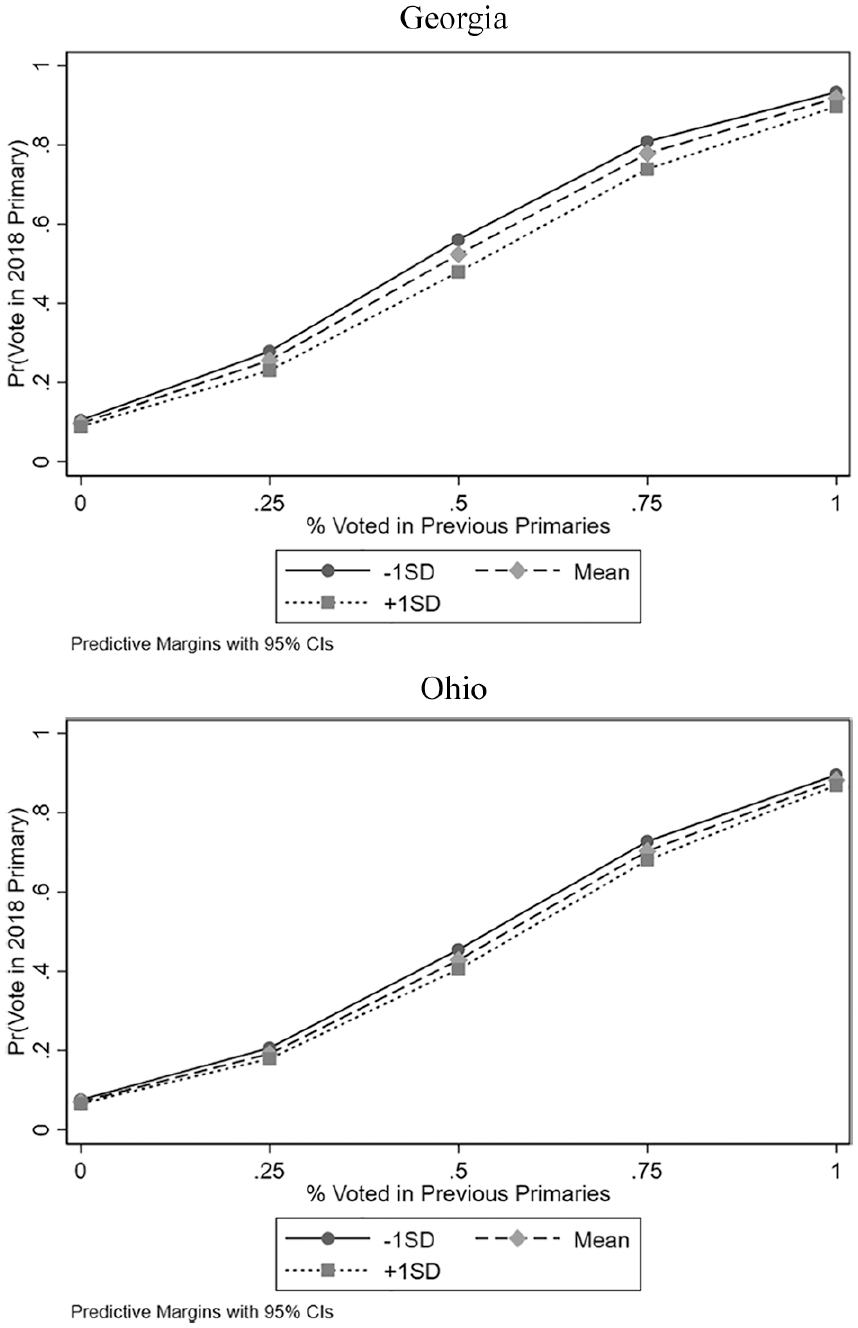
Predicted probabilities for the distance model: Georgia and Ohio.

These results show that living closer to a gubernatorial candidate increases the likelihood of turning out to the vote in the primary. The effect of distance looks quite similar to the effects of living in the same county as a candidate. Overall, these results bolster our argument that living in the same county or being more proximate in terms of actual distance leads to the largest increases in voter turnout.

Supplemental Analyses

Given the concentration of candidates in the Georgia gubernatorial primary from the Atlanta area, we provide an additional analysis for Georgia to see if the hometown effect holds up when focusing only on the Atlanta area. Table 4 and Figure 6 show the results for only registered voters living in the Atlanta Metropolitan Statistical Area (MSA). The Atlanta MSA consists of twenty counties and includes more than 2.9 million registered voters in the dataset. Of those voters, 42 percent in 2018 lived in a county with a hometown candidate. The results look similar to those presented above with the hometown effect being 1.9 percent for those without a primary voting history, 4.4 percent for those voting in 25 percent of previous primaries, 5.6 percent for those that have voted in half of the previous primaries, 3.5 percent for the 75 percent voters, and 1.4 percent for those that had turned out in all the previous primaries included in the dataset. These results show that the hometown effect we are seeing in Georgia is not simply an artifact of higher turnout in the Atlanta area or some other Atlanta-specific factor that could be driving turnout.

Table 4.

Turnout Model Results: Atlanta Metropolitan Area.

	Model 1: hometown
Hometown candidate^a	0.2115* (0.0042)
%Voted in previous primaries	4.9425* (0.0101)
Interactions
Hometown candidate × %Voted	0.0389* (0.0159)
Constant	−2.2948* (0.0028)
No. of observations	2,978,165

The dependent variable for this logistic regression is turnout with one indicating that the voter participated and zero indicating that they did not. Model 1 reports the effect of living in the same county as a gubernatorial candidate. The sample is restricted to only registered voters living in the Atlanta Metropolitan Statistical Area (MSA). Standard errors are given in parentheses.

No local candidate is the base category.

p < .001.

Figure 6.

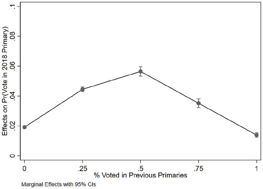
Marginal effects for hometown candidate: Atlanta Metropolitan Area.

Our results suggest a significant role for candidate geographic proximity on primary turnout conditional on previous primary voting history. The measure we employ for previous turnout is based on actual turnout over the length of the available data. This measure weighs all voters as the same regardless of their length of time living in a county and may not be fully accounting for the proclivity to vote. Theoretically, this may not be fully accounting for the potential friends and neighbors effect, as individuals living in a county longer may have more attachment to the area and be more likely to be nudged toward the voting booth by a local candidate. Therefore, we conduct one additional analysis that accounts for the length of time someone has been registered to vote in their county. We include this as a three-way interaction in the model and present the results in Table 5 and Figure 7.

Table 5.

Turnout Model Results by Length of County Registration.

	Model 1: Georgia	Model 2: Ohio
Hometown candidate^a	0.1938* (0.0048)	0.1367* (0.0045)
%Voted in previous primaries	6.7960* (0.0114)	4.8315* (0.0086)
Years registered in county	0.0058* (0.0002)	0.0083* (0.0002)
Interactions
Hometown candidate × %Voted	0.9560* (0.0273)	0.1597* (0.0122)
Hometown candidate × Years registered	0.0024* (0.0004)	−0.0066* (0.0002)
%Voted × Years registered	−0.0758* (0.0004)	−0.0179* (0.0003)
Hometown candidate × %Voted × Years registered	−0.0206* (0.0008)	0.0121* (0.0004)
Constant	−2.4119* (0.0025)	−2.7261* (0.0032)
No. of observations	6,064,161	6,817,139

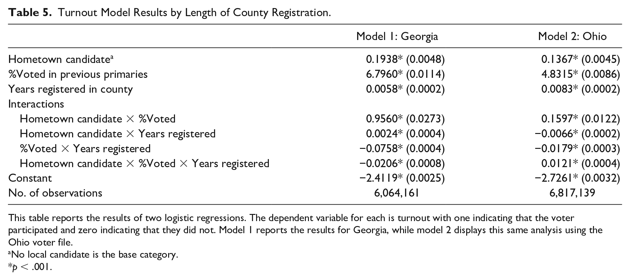
This table reports the results of two logistic regressions. The dependent variable for each is turnout with one indicating that the voter participated and zero indicating that they did not. Model 1 reports the results for Georgia, while model 2 displays this same analysis using the Ohio voter file.

No local candidate is the base category.

p < .001.

Figure 7.

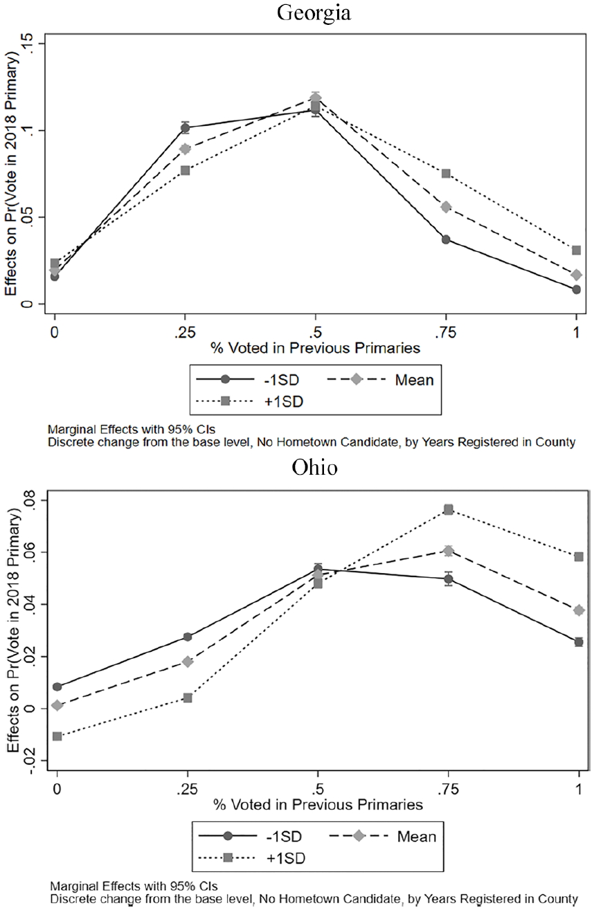
Marginal effects for a hometown candidate by length of registration in the county.

Figure 7 shows the marginal effects of having a hometown candidate across the likelihood of voting by length of county voter registration. In each state, we use the mean and ±1 standard deviation. In Georgia, the average voter had been registered for twelve years in their current county with a standard deviation of twelve years. We show the likelihood of voting by those newly registered in the county¹² (these individuals could have been registered to vote previously in the state), those registered for twelve years, and those for twenty-four years. In Ohio, the average voter had been registered for eighteen years in the county with a much larger standard deviation. We present results for those newly registered in the county, those registered for eighteen years, and those registered for forty-three years. These county registration averages make sense given the recent demographic changes in the states, with Georgia having a growing population and Ohio being a rust belt state with stagnant population growth.

The results in both states mirror the previous results across registration lengths. There is no difference in the length of registration for nonvoters in Georgia. In Ohio, while being substantively small, more long-time registrants are slightly less likely to turn out with a hometown candidate on the ballot compared with those without a hometown candidate. In both states, for those that had voted in 25 percent of previous primaries, a hometown candidate has a stronger effect on those newly registered voters; however, it is stronger for the more habitual voters who had been registered longer in the county. This makes sense with our theory as the 25 percent previous voters may not necessarily be nonvoters but are just new to the area and are, therefore, potentially miscoded in the data. This is especially so for any newly relocated residents from out of state, primarily in Georgia. For the occasional voter (50%), there is no difference in either state for length of registration. For the more habitual voters who have been registered in their county longer, a hometown candidate may be more central to them and provide a greater push to turnout.

Discussion

These results show a consistent and robust increase in primary turnout, primarily among those who occasionally vote in primary elections, when there is a home county or geographically proximate gubernatorial candidate. Our focus has been on home county candidates, but we acknowledge that the size, shape, and even topography of a state could play a role in how the “hometown effect” is diluted or magnified. For example, a three-county state such as Delaware or some western states with sparsely populated counties might see a diluted proximity effect (Pearson-Merkowitz and McTague 2008). The distance measure or a version that accounts for the state’s size may be most appropriate when comparing across states of various geographies and political boundaries.

The importance of geographic proximity is also likely to vary across electoral and campaign contexts. We argue that this effect provides an additional informational cue that may be more attenuated or magnified, depending on the myriad of other campaign and electoral cues in a given state election cycle. In these findings, the effect is clearly stronger in Georgia than Ohio, and while we cannot directly account for this variation, we can offer some speculation. There is virtually no proximity effect in the Ohio Republican primary. Part of this may be due to the two Republican candidates both being statewide office holders. On the other hand, Georgia may highlight the context where geographic proximity can serve as an important driver with competitive, well-covered, and contentious primaries in both parties with candidates all living in the general area of the state’s major metropolitan center.

Conclusion

One of the most interesting puzzles for political scientists and practitioners is determining what, exactly, motivates voters to participate in elections. The literature on voter turnout has found that turnout can be influenced by, among other things, social pressure (Gerber, Green, and Larimer 2008), perceptions of institutional arrangements (Gerber et al. 2013), and campaigns (Arceneaux and Nickerson 2009). Our study adds to this body of work. Using voter rolls, we avoid the risk of ecological fallacy, or relying on survey data which, for a myriad of reasons, may not be accurate. We can conclusively state that voters in these states turned out in greater numbers when there is a home county candidate on the ballot. We are also able to analyze the type of voter—a habitual voter, an occasional voter, or a nonvoter—that is most impacted by the presence of a home county candidate. We find, in both states, that it is the occasional voter who is most affected by the presence of a local candidate; however, there is also an uptick, albeit more modest, in turnout for the habitual voters.

This is logical; habitual voters who usually engage in politics are most likely to turn out regardless of who is running, but are also most likely to be aware of a hometown candidate. This additional cue seems to spur some additional turnout among this group. Nonvoters in previous primaries are unlikely to vote regardless of who is on the ballot, and may not even know or care who is on the ballot. A hometown candidate is unlikely to provide the knowledge or efficacy necessary for these nonvoters to bother turning out. For the occasional voters, whom may pay just enough attention to politics to realize that there is a hometown candidate on the ballot, the presence of a hometown candidate may provide a heuristic necessary to participate in the primary when they may not otherwise. This would be in keeping with the literature on the impact of education and information on voter turnout (Lassen 2005; Wolfinger and Rosenstone 1980).

These findings reinforce previous work that suggests a curvilinear effect for campaign or GOTV efforts as nonvoters are less likely to take notice or respond to campaign efforts, while habitual voters are going to vote regardless (Niven 2001, 2004). These occasional voters are most likely to respond to additional informational cues such as having a local candidate on the ballot.

We are also able to geocode our data to determine whether there is a substantive difference between how a voter behaves when a candidate from the same county is on the ballot and how a voter behaves depending on their actual geographic proximity to the gubernatorial candidate’s hometown. Our results are essentially the same whether we use the dichotomous home county variable or the distance variable, which should prove a useful finding for future scholars looking into the impact of the “friends and neighbors” effect.

Scholarship on friends and neighbors voting goes back more than seventy years. Political scientists have examined its effect using a variety of methods and sources of data and have consistently found that there is still a lot of utility to what Key posited in the 1940s. While much of Key’s work was rooted in a one-party era and focused on increases in vote share, we argue our results suggest that the current importance of a hometown effect may be more rooted in a mobilization rather than a persuasion effect. Given the strength of partisan attachments, it is unlikely that a local candidate is likely to move voters to vote against their partisanship, but provides an additional cue for pushing those occasional primary voters to the ballot box. Far from being a dated concept, there are still numerous facets to explore when it comes to the influence of proximity on voter turnout. Nonetheless, the media has paid scant attention to this explanatory variable. For example, media coverage of the Ohio and Georgia gubernatorial primaries in 2018 focused on factors such as race, public sentiment toward President Donald Trump, the power of out-of-state donors, and even the power of celebrity endorsements all the while ignoring the seemingly old-fashioned “friends and neighbors” effect. It is noteworthy that, even in the era of candidates trying to become social media superstars, and endless media prognostications about which candidate can best use new technology to capture voters’ imaginations, something as seemingly quaint as the presence of a “hometown candidate” can significantly increase voter turnout.

Footnotes

Acknowledgements

The authors thank the American Politics working group at the University of Mississippi, discussants at the 2018 The Citadel Symposium on Southern Politics, and the 2019 Southern Political Science Association Conference along with the editors at PRQ and three anonymous reviewers for their helpful feedback.

Declaration of Conflicting Interests

The author(s) declared no potential conflicts of interest with respect to the research, authorship, and/or publication of this article.

Funding

The author(s) received no financial support for the research, authorship, and/or publication of this article.

ORCID iDs

Jonathan Winburn

Mohammed Shariful Islam

Notes

References

Althaus

Scott L.

Trautman

Todd C.

2008. “The Impact of Television Market Size on Voter Turnout in American Elections.” American Politics Research 36 (6): 824–56.

Arceneaux

Kevin

Nickerson

David W.

2009. “Who Is Mobilized to Vote? A Re-analysis of 11 Field Experiments.” American Journal of Political Science 53 (1): 1–16.

Aspin

Larry T.

Hall

William K.

1989. “Friends and Neighbors Voting in Judicial Retention Elections: A Research Note Comparing Trial and Appellate Court Elections.” Western Political Quarterly 42 (4): 587–96.

Bardwell

Kedron

. 2002. “Money and Challenger Emergence in Gubernatorial Primaries.” Political Research Quarterly 55 (3): 653–68.

Bhatti

Yosef

Hansen

Kasper M.

2016. “The Effect of Residential Concentration on Voter Turnout among Ethnic Minorities.” International Migration Review 50 (4): 977–1004.

Black

Earl

Black

Merle

. 1973. “The Wallace Vote in Alabama: A Multiple Regression Analysis.” Journal of Politics 35 (3): 730–36.

Bowler

Shaun

Donovan

Todd

Snipp

Joseph

. 1993. “Local Sources of Information and Voter Choice in State Elections: Microlevel Foundations of the ‘Friends and Neighbors’ Effect.” American Politics Quarterly 21 (4): 473–89.

Brenner

Philip S.

DeLamater

John

. 2016. “Lies, Damned Lies, and Survey Self-reports? Identity as a Cause of Measurement Bias.” Social Psychology Quarterly 79 (4): 333–54.

Campbell

Angus

Converse

Philip

Miller

Warren

Stokes

Donald

. 1960. The American Voter. New York: Wiley.

10.

Campbell

James E.

Alford

John R.

Henry

Keith

. 1984. “Television Markets and Congressional Elections.” Legislative Studies Quarterly 9 (4): 665–78.

11.

Converse

Philip E.

1962. “Information Flow and the Stability of Partisan Attachments.” Public Opinion Quarterly 26 (4): 578–99.

12.

Cooper

Christopher

Knotts

H. Gibbs

Haspel

Moshe

. 2009. “The Content of Political Participation: Letters to the Editor and the People who Write Them.” PS: Political Science and Politics 42 (1): 131–37.

13.

Cutler

Fred

. 2002. “The Simplest Shortcut of All: Sociodemographic Characteristics and Electoral Choice.” Journal of Politics 64 (2): 466–90.

14.

Denny

Kevin

Doyle

Orla

. 2009. “Does Voting History Matter? Analysing Persistence in Turnout.” American Journal of Political Science 53 (1): 17–35.

15.

Downs

Anthony

. 1957. An Economic Theory of Democracy. New York: Harper.

16.

Dudley

Robert L.

Rapoport

Ronald B.

1989. “Vice-Presidential Candidates and the Home State Advantage: Playing Second Banana at Home and on the Road.” American Journal of Political Science 33 (2): 537–40.

17.

Enos

Ryan

Fowler

Anthony

Vavreck

Lynn

. 2014. “Increasing Inequality: The Effect of GOTV Mobilization on the Composition of the Electorate.” Journal of Politics 76 (1): 273–88.

18.

Fenno

Richard

. 1978. Home Style: House Members in Their Districts. Boston: Little, Brown.

19.

Fowler

James H.

2006. “Habitual Voting and Behavioral Turnout.” Journal of Politics 68 (2): 335–44.

20.

Garand

James C.

1988. “Localism and Regionalism in Presidential Elections: Is There a Home State or Regional Advantage.” Western Political Quarterly 41 (1): 85–103.

21.

Garlick

Alex

. 2015. “‘The Letter after Your Name’: Party Labels on Virginia Ballots.” State Politics and Policy Quarterly 15 (2): 147–70.

22.

Gerber

Alan S.

Green

Donald P.

Larimer

Christopher W.

2008. “Social Pressure and Voter Turnout: Evidence from a Large-Scale Field Experiment.” American Political Science Review 102 (1): 33–48.

23.

Gerber

Alan S.

Green

Donald P.

Shachar

Ron

. 2003. “Voting May Be Habit Forming: Evidence from a Randomized Field Experiment.” American Journal of Political Science 47 (3): 540–50.

24.

Gerber

Alan S.

Huber

Gregory A.

Doherty

David

Dowling

Conor M.

Hill

Seth J.

2013. “Do Perceptions of Ballot Secrecy Influence Turnout? Results from a Field Experiment.” American Journal of Political Science 57 (3): 537–51.

25.

Gimpel

James G.

Karnes

Kimberly A.

McTague

John

Pearson-Merkowitz

Shanna

. 2008. “Distance-Decay in the Political Geography of Friends-and-Neighbors Voting.” Political Geography 27 (2): 231–52.

26.

Green

Donald P.

Shachar

Ron

. 2000. “Habit Formation and Political Behaviour: Evidence of Consuetude in Voter Turnout.” British Journal of Political Science 30 (4): 561–73.

27.

Kahn

Kim Fridkin

Kenney

Patrick J.

1999. “Do Negative Campaigns Mobilize or Suppress Turnout? Clarifying the Relationship between Negativity and Participation.” American Political Science Review 93 (4): 877–89.

28.

Kawai

Kei

Watanabe

Yasutora

. 2013. “Inferring Strategic Voting.” The American Economic Review 103 (2): 624–62.

29.

Key

V. O.

Jr.

1949. Southern Politics in State and Nation. New York: Knopf.

30.

Lassen

David Dreyer

. 2005. “The Effect of Information on Voter Turnout: Evidence from a Natural Experiment.” American Journal of Political Science 49 (1): 103–18.

31.

Lewis-Beck

Michael S.

Rice

Tom W.

1983. “Localism in Presidential Elections: The Home State Advantage.” American Journal of Political Science 27 (3): 548–56.

32.

Meredith

Marc

. 2013a. “Exploiting Friends-and-Neighbors to Estimate Coattail Effects.” American Political Science Review 107 (4): 742–65.

33.

Meredith

Marc

. 2013b. “Heterogeneous Friends-and-Neighbors Voting.” Working paper. University of Pennsylvania, Philadelphia.

34.

Morehouse

Sarah M.

1990. “Money versus Party Effort: Nominating for Governor.” American Journal of Political Science 34 (3): 706–24.

35.

Niven

David

. 2001. “The Limits of Mobilization: Turnout Evidence from State House Primaries.” Political Behavior 23 (4): 335–50.

36.

Niven

David

. 2004. “The Mobilization Solution? Face-to-Face Contact and Voter Turnout in Municipal Elections.” Journal of Politics 66 (3): 868–84.

37.

Panagopoulos

Costas

Leighley

Jan E.

Hamel

Brian T.

2017. “Are Voters Mobilized by a ‘Friend-and-Neighbor’ on the Ballot? Evidence from a Field Experiment.” Political Behavior 39 (4): 865–82.

38.

Pearson-Merkowitz

Shanna

McTague

Michael

. 2008. “Partisan Mountains and Molehills: The Geography of U.S. State Intraparty Factionalism.” State Politics and Policy Quarterly 8 (1): 7–31.

39.

Plutzer

Eric

. 2002. “Becoming a Habitual Voter: Inertia, Resources, and Growth in Young Adulthood.” American Political Science Review 96 (1): 41–56.

40.

Popkin

Samuel L.

1991. The Reasoning Voter: Communication and Persuasion in Presidential Campaigns. Chicago: University of Chicago Press.

41.

Rice

Tom W.

Macht

Alisa A.

1987a. “Friends and Neighbors Voting in Statewide General Elections.” American Journal of Political Science 31 (2): 448–52.

42.

Rice

Tom W.

Macht

Alisa A.

1987b. “The Hometown Advantage: Mobilization or Conversion?” Political Behavior 9 (3): 257–62.

43.

Stone

Walter J.

Maisel

L. Sandy

. 2003. “The Not-so-Simple Calculus of Winning Potential U.S. House Candidates’ Nomination and General Election Prospects.” Journal of Politics 65 (4): 951–77.

44.

Taebel

Delbert A.

1975. “The Effect of Ballot Position on Electoral Success.” American Journal of Political Science 19 (3): 519–26.

45.

Tatalovich

Raymond

. 1975. “‘Friends and Neighbors’ Voting: Mississippi, 1943-73.” Journal of Politics 37 (3): 807–14.

46.

Van Wingen

John R.

1984. “Localism, Factional Fluidity, and Factionalism: Louisiana and Mississippi Gubernatorial Contests.” Social Science History 8 (1): 3–41.

47.

Van Wingen

John R.

Parker

Joseph B.

1979. “Measuring Friends-and-Neighbors Voting.” American Politics Quarterly 7 (3): 367–83.

48.

Wolfinger

Raymond E.

Rosenstone

Steven J.

1980. Who Votes? New Haven: Yale University Press.