Factor Structure of the Maslach Burnout Inventory–Educators Survey in a Polish-Speaking Sample

Abstract

This article investigates the psychometric properties of a mainstream burnout measure dedicated to teachers: the Maslach Burnout Inventory–Educators Survey (MBI-ES). The study used data gathered from a random sample of 1,206 primary school teachers in Poland to verify the construct validity of the MBI-ES. Eight alternative measurement models suggested in the literature were tested using confirmatory factor analysis. Contrary to many previous studies, this study did not support the oblique three-factor structure of the MBI-ES. A bifactor model with one general Burnout factor and three specific orthogonal factors of personal accomplishment, depersonalization, and emotional exhaustion showed best fit to the data. Additional analyses supported the measure’s essential unidimensionality. The results yield theoretical implications for construct reconceptualization and practical guidelines for researchers and practitioners.

Keywords

Maslach Burnout Inventory–Educators survey (MBI-ES)job burnout confirmatory factor analysis (CFA)bifactor model teachers

Introduction

Job burnout is a syndrome of emotional exhaustion, depersonalization, and reduced personal accomplishment that may occur among individuals who experience chronic stress while working with people (Maslach, Jackson, & Leiter, 1996; Maslach, Schaufeli, & Leiter, 2001). It emerged as an important concept in the 1970s (Freudenberger, 1975; Maslach, 1976) and seems to be rooted in the transformation from an industrial society to a service economy, accompanied by the psychological pressures afflicting workers (Schaufeli, Leiter, & Maslach, 2009). Job burnout was identified as a universal phenomenon not limited to the Western world (Golembiewski, 1996). Numerous studies have shown that job burnout relates to other psychological constructs, is influenced by resources and job demands, and affects workers’ behavior or job performance. Despite a considerable body of knowledge about the nature, causes, and consequences of burnout, which provide valuable insights enabling practitioners to cope with, prevent, and combat job burnout, it remains a fundamental challenge of working life (Leiter, Bakker, & Maslach, 2014).

The Maslach Burnout Inventory (MBI, Maslach & Jackson, 1981; Maslach et al., 1996) is a mainstream burnout measurement tool available to researchers and practitioners for use with human services workers (MBI–Human Services Survey, MBI-HSS), teachers (MBI–Educators Survey, MBI-ES), and other professionals (MBI–General Survey, MBI-GS). Forms of the survey for students (MBI–Students Survey, MBI-SS; Schaufeli, Martinez, Pinto, Salanova, & Bakker, 2002) and patients (MBI–Patient Survey, MBI-PS; Mind Garden, n.d.) have also been developed. Each form comprises three subscales representing the syndrome’s dimensions: emotional exhaustion (EE), depersonalization (DP), and personal accomplishment (PA); although in the MBI-GS, DP was renamed cynicism and PA was renamed professional efficacy.

This study focuses on the MBI-ES form of the survey. This is a 22-item measure of teacher burnout that originated from MBI-HSS through changing the word “recipient” to “student”. The items describe feelings and situations regarding work (e.g., “I feel depressed at work.”) and require respondents to rate how often they experience them on a 7-point scale ranging from 0 (never) to 6 (every day).

The popularity of the MBI is reflected in numerous studies on its psychometric properties (for meta-analyses, see Aguayo, Vargas, de la Fuente, & Lozano, 2011; Worley, Vassar, Wheeler, & Barnes, 2008). Among those investigating the construct validity of the MBI-ES (see Table 1) and MBI-HSS (e.g., Loera, Converso, & Viotti, 2014; Richardsen & Martinussen, 2004; Vanheule, Rosseel, & Vlerick, 2007), almost all have indicated the three-factor structure as best fitting to the data.

Table 1.

Review of Selected Studies on MBI-ES (2000–2016).

Paper	Country	Sample (n)	Sampling (Response Rate)	Reliability	Analyses	Final Model (s)
Aluja, Blanch, and Garcia (2005)	Spain	Elementary school teachers (631)	n.s. (n.s.)	α_EE = .83 α_DP = .50 α_PA = .79	EFA orthogonal, EFA oblique, CFA	EFA 3f: 43% of variance explained, cross-loadings present, latent correlations: r _{EE_PA} = −.22; r _{EE_DP} = .22; r _{DP_PA} = −.18 CFA 3f (Items 1, 16, 14, 7, and 12 excluded), χ² _ML (116) = 249.50***; CFI = .76; GFI = .92; AGFI = .89; NFI = .64; RMSEA = .04; ECVI = .51, latent correlations: r _{EE_PA} = −.49; r _{EE_DP} = .59; r _{DP_PA} = −.39
Chigerwe, Boudreaux, and Ilkiw (2014)	United States	Veterinary students (170)	Convenience (53%)	α_EE = .60 α_DP = .52 α_PA = .77	EFA oblique	EFA 3f: Percentage of variance explained n.s., cross-loadings present, latent correlations: r _{EE_PA} = −.20; r _{EE_DP} = .63; r _{DP_PA} = −.23
Denton, Chaplin, & Wall (2016)	United States, Jamaica	Elementary and secondary school teachers (300)	Convenience (n.s.)	n.s.	EFA oblique, CFA, multigroup CFA	EFA 3f: Jamaica: 53%, United States: 58% of variance explained, cross-loadings present, latent correlations n.s. CFA 3f (6 EE items moved to DP): Jamaica: χ² _ML (206) = 398.48**; CFI = .80; TLI = .78; RMSEA = .08; United States: χ² _ML* (206) = 462.43**; CFI = .81; TLI = .79; RMSEA = .09, latent correlations: n.s. CFA unconstrained multigroup 3f (Items 6, 14, 16, 20, 10, 15, 22, and 12 excluded): χ² _ML* (109) = 180.98***; CFI = .93; TLI = .91; RMSEA = .07, latent correlations Jamaica: r_{EE_PA} = −.09; r_{EE_DP} = −.47; r_{DP_PA} = −.09; United States: r _{EE_PA} = −.31; r _{EE_DP} = −.66; r _{DP_PA} = −.16
Kokkinos (2006)	Cyprus	Elementary and secondary school teachers (771)	Random at school level (48%)	α_EE = .85 α_DP = .63 α_PA = .71 α_all = .74	EFA orthogonal, EFA oblique, CFA	EFA 3f: 52% of variance explained, cross-loadings present, latent correlations n.s., raw scores correlations: r _{EE_PA} = −.09; r _{EE_DP} = .38; r _{DP_PA} = −.35 CFA 3f: χ² _ML (206) = 978.64***; CFI: .83; RSMEA = .08; SRMR = .08, latent correlations n.s.
Lundkvist, Stenling, Gustafsson, & Hassmén (2014)	Sweden	Sport coaches (277)	Convenience (46%)	n.s.	CFA	CFA 3f (Items 12, 16, 20 excluded): χ² _WLSMV (149) = 393.49***; CFI = .94; TLI = .93; RMSEA = .08, latent correlations: r _{EE_PA} = −.26; r _{EE_DP} = .77; r _{DP_PA} = −.46
Schwarzer, Schimitz, & Tang (2000)	Hong Kong, Germany	Teachers (Hong Kong: 261, Germany: 257)	n.s. (n.s.)	Germany: α_EE = .88 α_DP = .69 α_PA = .82 Hong Kong: α_EE = .88 α_DP = .79 α_PA = .83	EFA orthogonal	EFA 3f: Hong Kong: 55%, Germany: 51% of variance explained, cross-loadings present, latent correlations n.s., raw scores correlations: Hong Kong: r _{EE_PA} = .12; r _{EE_DP} = .66; r _{DP_PA} = −.02; Germany: r _{EE_PA} = −.40; r _{EE_DP} = .58; r _{DP_PA} = −.45
Van Droogenbroeck, Spryut, & Vanroelen (2014)	Belgium	Senior teachers (1878)	Random at teachers level (62%)	α_EE = .89 α_DP = .82 α_PA = .81	CFA	CFA 3f (cross-loading and errors correlation allowed, details n.s.): χ² _MLM (101) = 319.63***; RMSEA = .04; CFI = .97; TLI = .97; SRMR = .03, latent correlations n.s., raw score correlations: r _{EE_PA} = −.29; r _{EE_DP} = .74; r _{DP_PA} = −.38
van Horn (2002)	Netherlands	Teachers (1629)	Mixed samples both convenience and random either at school or teachers level (27–76%)	α_EE = .90 α_DP = .72 α_PA = .82	CFA	CFA 3f (two extra items): χ²(206) = 2135.33***; NNFI: .87; GFI = .89; AGFI = .86; RMSR = .10, latent correlations n.s., raw scores correlations: r _{EE_PA} = −.17; r _{EE_DP} = .42; r _{DP_PA} = −.38
Whitehead, Ryba, & O’Driscoll (2000)	New Zealand	Primary school teachers and principals (386)	n.s. (n.s.)	α_EE = .90 α_DP = .79 α_PA = .77	EFA oblique	EFA 3f: 51% of variance explained, cross-loadings present, latent correlations: r _{EE_PA} = −.18; r _{EE_DP} = .48; r _{DP_PA} = −.37

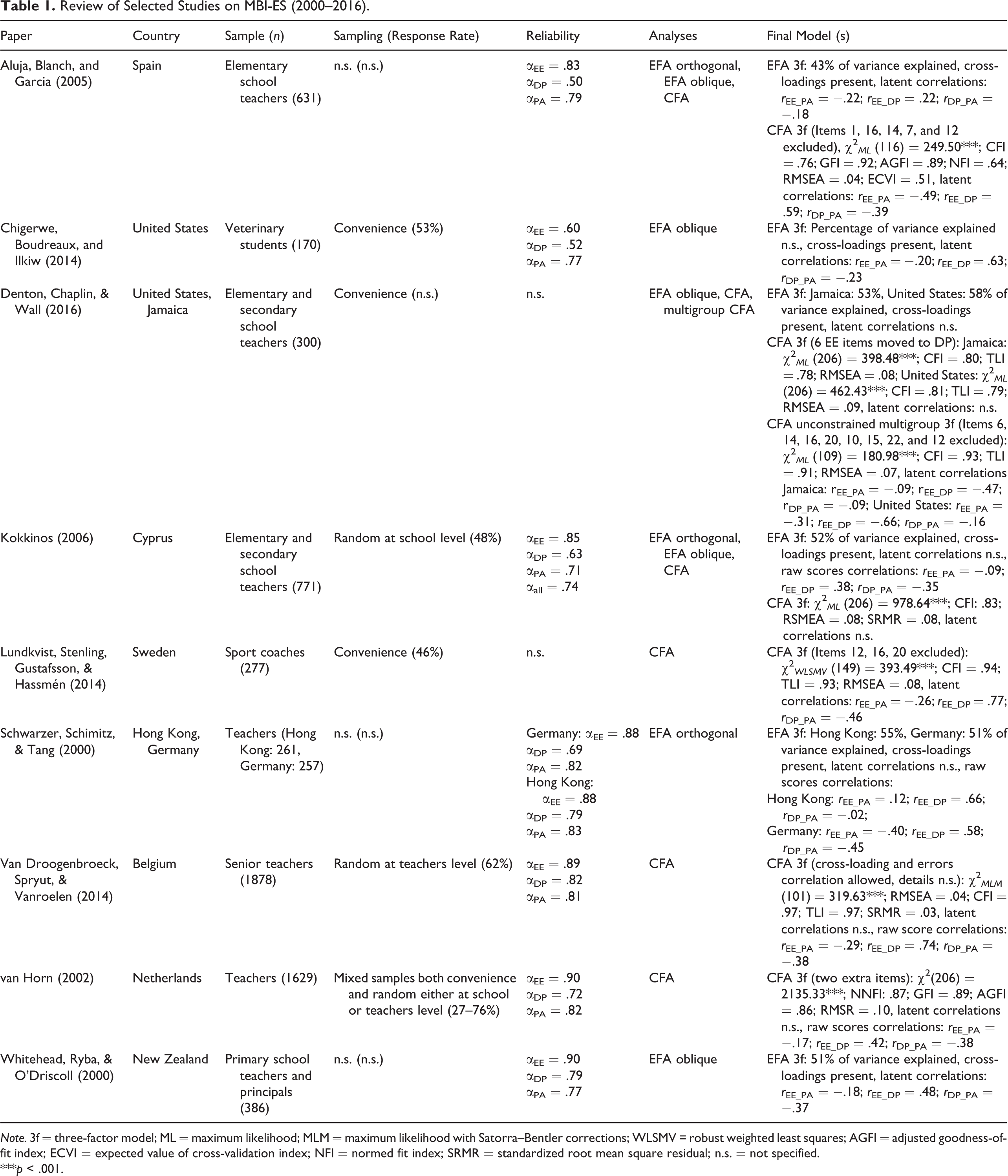
Note. 3f = three-factor model; ML = maximum likelihood; MLM = maximum likelihood with Satorra–Bentler corrections; WLSMV = robust weighted least squares; AGFI = adjusted goodness-of-fit index; ECVI = expected value of cross-validation index; NFI = normed fit index; SRMR = standardized root mean square residual; n.s. = not specified.

***p < .001.

These results, although they are coherent, share several shortcomings. First, although the three-factor structure held, the model fit indices did not necessarily meet currently recommended thresholds (Hu & Bentler, 1999). For example, an examination of Table 1 shows that only two of six confirmatory factor models with reported root mean square error of approximation (RMSEA) had an RMSEA value that fell below .06. Only one of six models with reported comparative fit index (CFI) had CFI value that reached the recommended .95 threshold. Similar results were obtained for the MBI-HSS (see Loera et al., 2014, for review).

Second, some researchers modified their models to obtain acceptable fit. Such modifications were less common for the MBI-ES or MBI-HSS than for other forms. Typical modifications of the MBI three-factor structure included allowing error covariances (e.g., Kitaoka-Higashiguchi et al., 2004; Langballe, Falkum, Innstrand, & Aasland, 2006; Mäkikangas, Hätinen, Kinnunen, & Pekkonen, 2011; Schutte, Toppinen, Kalimo, & Schaufeli, 2000, in the MBI-GS and Hu & Schaufeli, 2009, in the MBI-SS) or cross-loadings (Van Droogenbroeck, Spruyt, & Vanroelen, 2014, in the MBI-ES; Langballe et al., 2006, in the MBI-GS), shifting items between subscales (e.g., Denton, Chaplin, & Wall, 2016, in the MBI-ES) or deleting poorly performing items (e.g., Aluja, Blanch, & García, 2005; Byrne, 1993, in the MBI-ES; Pisanti, Lombardo, Lucidi, Violani, & Lazzari, 2013; Vanheule et al., 2007 in the MBI-HSS; Bria, Spânu, Băban, & Dumitraşcu, 2014, in the MBI-GS; Campos, Zucoloto, Bonafé, Jordani, & Maroco, 2011, in the MBI-SS). The cross-loadings of Items 12 and 16 observed in many studies prompted the authors of the MBI to recommend skipping them (Maslach et al., 1996).

Difficulties in restoring the three-factor structure of the MBI-ES and MBI-HSS resulted in a search for alternative models. Some researchers suggested a two-dimensional structure for the MBI-HSS: EE combined with DP and PA (e.g., Brookings, Bolton, Brown, & McEvoy, 1985; Dignam, Barrera, & West, 1986). Others split selected dimensions which resulted in four-factor models. Firth, Mcintee, Mckeown, and Britton (1985) suggested for the MBI-HSS that EE should comprise two dimensions: discouragement about work and emotional draining. Gil-Monte (2005), in the MBI-HSS, split PA into self-competence and existential component, whereas Chao, McCallion, and Nickle (2011), also in the MBI-HSS, divided DP into indifference about the care recipient and rejection of the care recipient. Iwanicki and Schwab (1981) separated DP in the MBI-ES form into job-related and student-related factors. Densten (2001) even suggested for the MBI-HSS a five-dimensional structure, with EE broken down into psychological strain and physical strain factors and PA split into PA related to self and PA related to other factors.

Although Maslach and Jackson (1981) initially described EE, DP, and PA as independent dimensions of burnout syndrome and used orthogonal rotations in factor analyses, some researchers considered burnout a unidimensional construct (e.g., Golembiewski & Munzenrider, 1981; Shirom, 1989). Moreover, repeatedly reported correlations between subscales of the different forms of the MBI (see Table 1 and Loera et al., 2014; Worley et al., 2008, for reviews) and better fit of the oblique confirmatory models in comparison to orthogonal ones (see Loera et al., 2014, for results on the MBI-HSS; Schutte et al., 2000, on the MBI-GS; van Horn, 2002, on the MBI-ES) resulted in recommendations for a higher order factor structure. Boles, Dean, Ricks, Short, and Wang (2000) proposed for the MBI-HSS a second-order model with three first-order factors (EE, DP, and PA) loading on a second-order factor representing general job burnout. An alternative approach to representing a general construct, comprising several highly related domains, is the bifactor model. In the bifactor model, each item loads both on (a) one general factor, accounting for variance shared by all the items and on (b) one of several specific facets, accounting for variance shared by a subset of items that is over and above the general factor. All the factors are uncorrelated (Holzinger & Swineford, 1937; see Figure 1). Mészáros, Ádám, Szabó, Szigeti, and Urbán (2014) found that the bifactor model for the MBI-HSS fitted data better than other models, including the oblique three-factor one. These results have not yet been replicated for any MBI form. Selected representations of burnout factorial structure available in the literature are graphically presented in Figure 1.

Figure 1.

Selected models of factorial structure of Maslach Burnout Inventory-Human Services Survey (MBI-HSS) and Maslach Burnout Inventory-Educators Survey (MBI-ES). Note. JB = general job burnout factor; EE = emotional exhaustion; DP = depersonalisation; PA = personal achievement. In the first-order three-factor oblique model (proposed by Maslach, 1981, for MBI-HSS), the relationships between first-order factors are modeled via covariances. In the second-order factor model (proposed by Boles et al., 2000, for MBI-HSS), the relationships between first-order factors are modeled via introduction of the second-order factor. This model is equivalent to first-order three-factor oblique model. In the bifactor model (proposed by Mészáros et al., 2014, for MBI-HSS), no relationships between first-order factors are assumed; the second source of variance is considered and consumed by the general burnout factor.

To summarize, despite the abundance of research, the MBI factor structure remains a source of considerable debate. Although many studies have supported the three-factor solution, the necessary modifications and often marginally acceptable fit have undermined these results. Meanwhile, suggestions for promising alternative models have not gained the recognition of scholars.

This study investigates the construct validity of the Polish-language version of the MBI-ES. It contributes to the discussion on MBI factor structure through testing various models suggested in the literature, including one recently proposed for the MBI-HSS and not-yet-replicated bifactor model (Mészáros, Ádám, Szabó, Szigeti, & Urbán, 2014). Moreover, to our knowledge, this is the first published study on the MBI-ES as administered to a Polish-speaking sample. The MBI-ES Polish-language version license vendor provides no information on its psychometric properties, and to date, no study inquiring into them has been published. This situation strongly precludes the wider use of the MBI-ES on Poles both for research and diagnostic purposes.

Method

Data and Sample

This study uses data from the Educational Value-Added for Primary Schools (EVA-PS) longitudinal study run between 2009 and 2015 in Poland. Over 5,500 students from 180 schools, along with their parents, teachers, and school principals, participated in the study. The EVA-PS focused on student achievement predictors, including teacher effect; thus, students were sampled first and the teachers’ sample depended on the students’ sample. Stratified two-stage cluster sampling was performed on students. First, public primary schools were split into strata based on their location (village, town, and city) and the number of Grade 1 classes in a school. Special education schools and schools with only one Grade 1 class of fewer than 10 students were excluded from the sampling frame. Within strata, schools were selected randomly with a probability proportional to the number of students in Grade 1 classes. Second, two Grade 1 classes were sampled from each school (if a school ran only one or two Grade 1 classes, all classes were sampled). It should be noted that a class is a stable group of students taught by different teachers for each subject. Students in Grade 1 in Poland are 7 years old.

Teachers of Polish (21%), mathematics (21%), natural sciences (18%), history and civic education (16%), and foreign language (25%), who taught the sampled classes, completed the MBI-ES in March and April 2014, when their students were in Grade 6 (fifth wave of the study). The response rate reached 96%. The analyses included data on 1,206 teachers from 179 schools (one school was closed down during the course of the study). Full-time teachers comprised 86% of the sample. Average teaching experience was 20 years.

Distribution of gender and distribution of the rank of professional promotion were close to distributions in the population of primary school teachers. Females comprised 91% of the sample and 87% of the population (Central Statistical Office, 2014). In the sample, 2% of teachers were trainees, 10% were contractual, 24% appointed, and 64% chartered teachers, while nationwide the figures were 2%, 13%, 26%, and 58%, respectively.¹ Other sample characteristics could not be checked against their distributions in the population due to lack of publicly available data.

Data Analysis

First, we ran a series of confirmatory factor analyses (CFA) to test the MBI-ES factorial structures described in the literature (see Introduction section and Table 3). We skipped the four-factor orthogonal structure proposed by Firth et al. (1985) because previous studies have shown that MBI dimensions are strongly correlated (see Table 1). We omitted exploratory factor analysis (EFA), since past studies allowed for the identification of possible factorial structures. Next, we compared computed models based on fit indices and chose a final solution that underwent additional analyses. We checked for possible cross-loadings, verified dimensionality, and factors’ reliability.

Model fit was assessed with three commonly used (McDonald & Ho, 2002) fit indices, that is, RMSEA, CFI, and the Tucker–Lewis index (TLI). We assumed that CFI and TLI values not lower than .95, and RMSEA values not higher than .06 indicated good fit (Hu & Bentler, 1999).

All the analyses were performed in Mplus 7.4 (Muthén & Muthén, 1998–2012) using the robustweighted least square (WLSMV) estimator, recommended for ordered categorical data (e.g., Flora & Curran, 2004). The models accounted for the nonindependence of teachers clustered within schools by adjusting to the standard errors using a sandwich estimator (Muthén & Muthén, 1998–2012; Muthén & Satorra, 1995).² The scales of latent variables were set by fixing their variances to unity.

Results

Table 2 presents descriptive statistics and correlations of subscales’ raw scores. Higher scores on the respective subscales denote higher levels of EE, DP, and PA.

Table 2.

MBI-ES Descriptive Statistics, Correlations, and Internal Consistencies.

Subscale	N _items	Mean	SD	Skewness	Kurtosis	Max	α	DP	PA
EE	9	13.74	9.93	1.09	1.06	52	.91	.54	−.43
DP	5	2.73	3.39	1.98	4.84	23	.70		−.39
PA	8	38.69	6.51	−0.95	1.52	48	.81

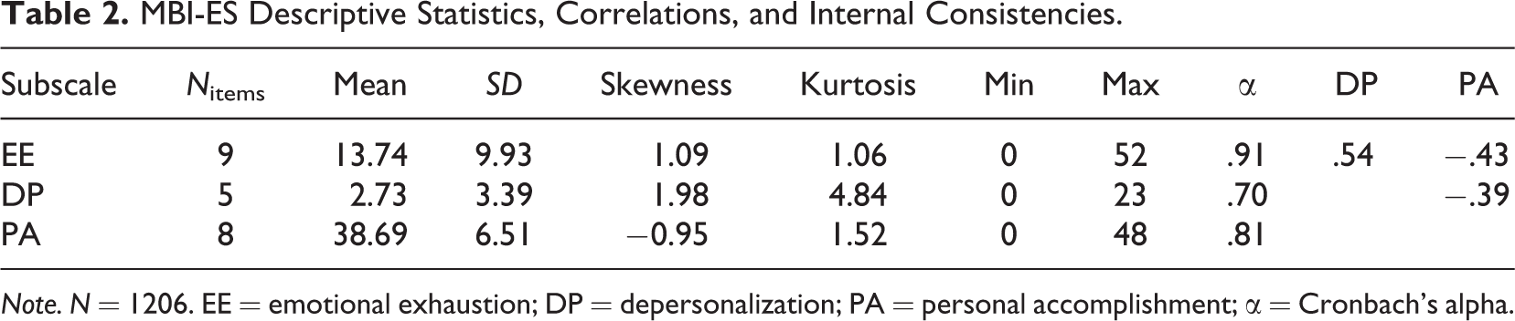
Note. N = 1206. EE = emotional exhaustion; DP = depersonalization; PA = personal accomplishment; α = Cronbach’s alpha.

Table 3 contains information on the tested CFA models and their fit. We started the examination from the M3a model, representing the original MBI-ES structure. The model fitted data poorly, as all reported fit indices did not meet the satisfactory values. Models nested in the M3a, but including fewer dimensions (M2, M1), showed even poorer fit. Two-factor M2 model had significantly poorer fit compared to M3a, Δχ²(1) = 129.58, p < .001, and the one-factor M1 model had significantly poorer fit compared to M2, Δχ²(1) = 359.16, p < .001. The three-factor M3a model fit data significantly more poorly in comparison to the four-factor M4a, Δχ²(3) = 55.23, p < .001, having the DP dimension divided into indifference and rejection. Despite the M4a model fitting data slightly better when contrasted to the M3a, it was rejected because two (RMSEA and TLI) of three fit indices did not meet the expected values.

Table 3.

Summary of the Tested Models.

Model	Description	Source	N _items	Subscales: Items	N _par	χ²(df)	RSMEA	CFI	TLI
M1	One factor		22	NA	153	4,186.53 (210)	.126	.855	.840
M2	Two-factor oblique	Brookings et al. (1985)	22	EE + DP: 1, 2, 3, 5, 6, 8, 10, 11, 13, 14, 15, 16, 20, 22; PA: 4, 7, 9, 12, 17, 18, 19, 21	155	260.30 (208)	.090	.925	.917
M3a	Three-factor oblique	Maslach (1981)	22	EE: 1, 2, 3, 6, 8, 13, 14, 16, 20; DP: 5, 10, 11, 15, 22; PA: 4, 7, 9, 12, 17, 18, 19, 21	157	1,612.58 (206)	.075	.949	.943
M3b	Three-factor oblique (12, 16 deleted)	Maslach et al. (1996)	20	EE: 1, 2, 3, 6, 8, 13, 14, 20; DP: 5, 10, 11, 15, 22; PA: 4, 7, 9, 17, 18, 19, 21	143	1,042.45 (167)	.066	.965	.960
M4a	Four-factor oblique	Chao et al. (2011)	22	EE: 1, 2, 3, 6, 8, 13, 14, 16, 20; DP_I: 5, 15, 22; DP_R: 10, 11; PA: 4, 7, 9, 12, 17, 18, 19, 21	160	1,571.68 (203)	.075	.950	.943
M4b	Four-factor oblique (12, 16 deleted)	Gil-Monte (2005)	20	EE: 1, 2, 3, 6, 8, 13, 14, 20; DP: 5, 10, 11, 15, 22; PA1: 4, 7, 17, 21; PA2: 9, 18, 19	146	006.52 (164)	.065	.966	.961
M5	Five-factor oblique (12, 13, 14 deleted)	Densten (2011)	19	EE_PS: 1, 2, 3, 8; EE_SS: 8, 16, 20; DP: 5, 10, 11, 15, 22; PA_S: 4, 9, 18, 19; PA_O: 7, 17, 21	143	1,030.16 (142)	.072	.959	.951
Mbf	Bifactor	Mészáros et al. (2014)	22	EE: 1, 2, 3, 6, 8, 13, 14, 16, 20; DP: 5, 10, 11, 15, 22; PA: 4, 7, 9, 12, 17, 18, 19, 21; JB: 1-22	176	716.36 (187)	.048	.981	.986

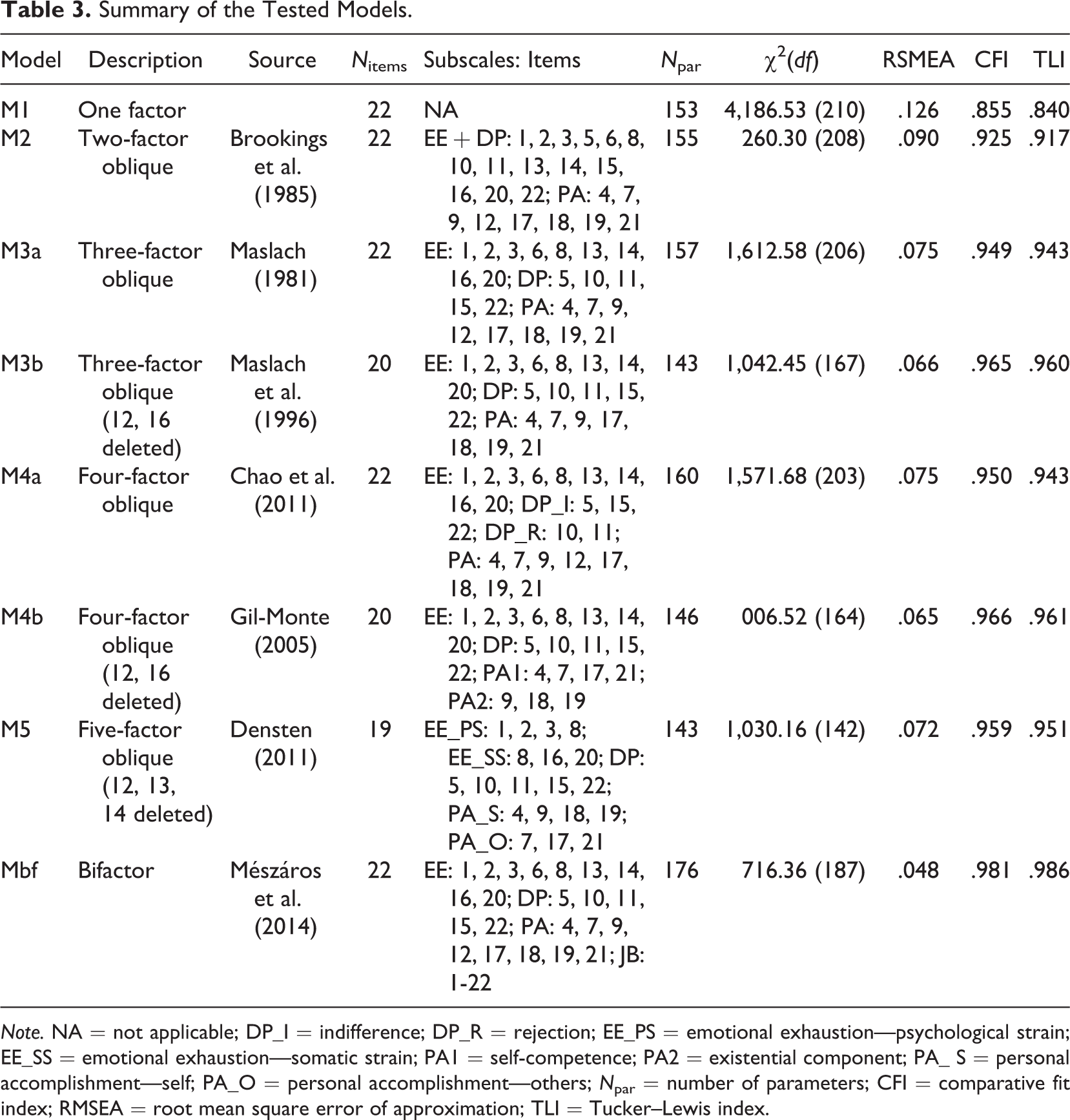
Note. NA = not applicable; DP_I = indifference; DP_R = rejection; EE_PS = emotional exhaustion—psychological strain; EE_SS = emotional exhaustion—somatic strain; PA1 = self-competence; PA2 = existential component; PA_ S = personal accomplishment—self; PA_O = personal accomplishment—others; N _par = number of parameters; CFI = comparative fit index; RMSEA = root mean square error of approximation; TLI = Tucker–Lewis index.

The Mbf model showed the best fit measured with RMSEA, CFI, and TLI in comparison to three-, four-, and five-factor oblique models. The M3a model, nested in Mbf, showed significantly poorer fit, Δχ²(19) = 609.27, p < .001. However, as shown by Murray and Johnson (2013) in their simulation study, bifactor models tend to show superior fit over higher order models and therefore first-order oblique factor models, not because they better represent latent structures but because they better accommodate unmodeled data complexity. Cross-loadings and error covariances have been allowed in many studies on the MBI as means to improve model fit (see Table 1), which suggests that the MBI-ES may have a complex factorial structure. Thus, there are two possible reasons for the better fit of the bifactor model. First, the bifactor may indeed better represent the MBI-ES latent structure, and modifications of the original structure observed in studies may have stemmed from forcing the data into an inappropriate model. The second reason refers to the possibility of the MBI-ES having a complex factorial structure. In this case, both models may be inappropriate because both assume the simple structure, that is, each item in the three-factor oblique model loaded on one and only one factor, and each item in the bifactor model loaded on the general factor and one and only one specific factor. However, the bifactor better accommodated the unmodeled complexity, which possibly resulted in its better fit.

To assess whether unmodeled complexity was responsible for the superior fit of the bifactor model, we specified a series of target-rotated bifactor models. These models allowed us to verify whether the MBI-ES had a complex latent structure after controlling for all items’ shared variance, that is, whether its items loaded on more than one specific factor. If they did, it would undermine the choice of the bifactor as better representing the MBI-ES latent structure. Exploratory structural equation modeling with target rotation is situated between the exploratory and the confirmatory approaches. It requires the specification of a target matrix of loadings based on partial knowledge about the factor structure (usually, loadings expected to be zero are indicated). The target loadings influence the rotation but, as they are not constrained, may finally end up with nonzero values if zero values do not provide satisfactory fit to the data (Asparouhov & Muthén, 2009; Browne, 2001). Thus, target rotation allows the easy identification of misspecified loadings.

To assure an adequate recovery of model parameters, we followed Moore, Reise, Depaoli, and Haviland’s (2015) iterative procedure. The authors demonstrated in their simulation study that this procedure allows for the recovery of true model parameters and outperforms the noniterative one. However, in the first step, we used a loadings matrix based on the MBI original factor structure (M3a) instead of an empirically based loadings matrix derived from EFA with a rotation from the Crawford-Ferguson family. After running the model, we updated the matrix by setting as zeros all loadings below .15. The cut-off criterion is low enough to assure nonsalience of potential cross-loadings (see McDonald, 1999). All loadings above the cut-off criterion were left unconstrained. We used the updated matrix in the estimation of the subsequent model. The procedure ended when no loading specifications in the target matrix could be modified.

Table 4 presents factor loadings for the final target-rotated bifactor model. The model fitted data well, χ²(146) = 515.50; p < .001; RMSEA = .045; CFI = .987; TLI = .979.

Table 4.

Factor Loadings of the Bifactor and Final Target-Rotated Bifactor Models.

Item	Target-Rotated Bifactor				Bifactor
Item	GEN	EE	DP	PA	GEN	EE	DP	PA
MBI1	.694*	.520*	.019	.053*	.663*	.567*
MBI2	.564*	.610*	−.078*	.021	.521*	.665*
MBI3	.650*	.475*	.004	.023	.634*	.498*
MBI6	.831*	.141*	−.094*	.047*	.767*	.241*
MBI8	.755*	.471*	.077*	−.006	.776*	.442*
MBI13	.731*	.433*	.074*	−.022*	.753*	.404*
MBI14	.505*	.418*	.001	.068*	.470*	.463*
MBI16	.705*	−.060	−.088*	.043	.643*	.055
MBI20	.714*	.476*	.013	.038	.701*	.492*
MBI5	.573*	−.060	.282*	−.111*	.589*		.246*
MBI10	.608*	.028	.590*	−.029	.637*		.594*
MBI11	.676*	.129*	.559*	−.033	.747*		.456*
MBI15	.557*	−.145*	.290*	−.065*	.520*		.323*
MBI22	.468*	−.008	.207*	−.072*	.490*		.151*
MBI4	−.304*	.106*	.007	.603*	−.264*			.647*
MBI7	−.370*	.089*	−.104*	.621*	−.349*			.648*
MBI9	−.379*	−.062*	−.074*	.594*	−.422*			.555*
MBI12	−.614*	−.198*	.057*	.416*	−.699*			.332*
MBI17	−.487*	.132*	.039	.482*	−.436*			.516*
MBI18	−.562*	−.073*	−.018	.508*	−.596*			.476*
MBI19	−.426*	−.062*	−.060*	.559*	−.466*			.525*
MBI21	−.543*	.042	−.017	.277*	−.526*			.289*

Note. Items belonging to respective MBI-ES subscales are in boldface. GEN = general burnout factor; EE = specific emotional exhaustion factor; DP = specific depersonalisation factor; PA = specific personal accomplishment factor; MBI-ES = Maslach Burnout Inventory–Educators Survey.

*p < .05.

Inspection of the factor loadings revealed that all items loaded significantly on the general job burnout factor. Loadings’ absolute values ranged from .30 (Item 4) to .83 (Item 6) and were higher on the general factor than on specific factors in the case of items building EE and DP subscales. Five of 8 items from DP subscale loaded stronger on the specific factor than on the general one. Seven items (4, 5, 7, 11, 12, 15, and 17) had absolute cross-loadings’ values of .10 or higher, with only Item 12 exceeding the value of .15 (−.198). All specific factor loadings of Items 6 and 16 were below .15. Observed cross-loadings were relatively small. Although some items showed statistically significant cross-loadings, they were low enough to be considered trivial (McDonald, 1999). Thus, we find them not to be a serious source of unmodeled complexity that could be responsible for the better fit of the bifactor model compared to the confirmatory three-factor oblique one.

To further explore the bifactor model (Mbf), we calculated several indices of the “strength” of the general and specific factors that serve for dimensionality assessment, that is, explained common variance (ECV), and omega-type reliability coefficients (omega, omegaH, and omegaS). The ECV shows how much total common variance is explained by the general factor. Values greater than .60 suggest unidimensionality, as there is not much common variance beyond the general factor (Reise, Moore, & Haviland, 2010). The proportion of the total score variance attributable to all common factors is expressed by omega, the proportion attributable to a general factor by omegaH. OmegaS is a measure of the unique reliability of each subscale after controlling for the general factor (see Reise, Bonifay, & Haviland, 2013, for detailed description).

ECV equaled .62, slightly exceeding the borderline value. The omega coefficients of .95 (all items), .94 (EE), .83 (DP), and .88 (PA) indicated that the general and specific factors reliably measured the blend of burnout facets. The general factor was also a reliable measure of a single latent variable, as its omegaH equaled .79. Its omegaH–omega ratio showed that that 83% of the reliable variance in the total score was due to general factor variation. OmegaS values for EE, DP, and PA equaled .28, .21, and .47, respectively, indicating low subscale reliability after controlling for the general factor. Subscale scores provided little reliable information distinct from the general factor. Indeed, omegaS–omega ratios showed that, respectively, 29%, 26%, and 53% of EE, DP, and PA reliable variance was attributable to specific factors.

These results suggest that the MBI-ES, although not strictly unidimensional as specific facets are observed, is essentially unidimensional. This means that “the dominant factor is so strong that trait level estimates are unaffected by (or are ‘robust to’) the presence of smaller specific factors and influences” (Embretson & Reise, 2013, p. 230).

Discussion

This study inquired into the construct validity of the MBI-ES. It aimed at identifying the MBI-ES factor structure in a Polish-speaking sample. The authors used CFA to test eight different factor structures suggested in the literature and subjected the best-fitting model to further detailed investigation.

Contrary to many previous studies on different forms and language versions of the MBI, this study did not support the oblique three-factor model. However, we do not find this result surprising. In many studies, such a model required several modifications to reach acceptable fit, which included allowing cross-loadings and error covariances, deleting items, or shifting items between subscales (as mentioned in the Introduction). In other studies, the original structure was modified through merging or splitting burnout dimensions. It must be noted that such modifications of the model have often been driven by a desire to obtain a better fit, without any theoretical justification. As such, they may have an undesirable impact on the coherence of the measured theoretical construct and may hinder comparisons between studies and results interpretation. For example, error covariances produce multidimensional factor scores that are difficult to interpret. The common difficulties in restoring the oblique three-factor model suggest, in our opinion, that other factorial structures should be considered.

Our analyses showed the best fit of the bifactor model in comparison to other models suggested in the literature. Moreover, this model did not require any of the above-mentioned modifications; in particular, skipping Items 12 and 16 due to cross-loadings, as suggested by the scale authors (Maslach et al., 1996), was no longer necessary.

Based on our results, we argue that cross-loadings and error covariances in the oblique three-factor structure reported in past studies may have stemmed from the influence of the common latent factor. Researchers partially modeled this influence through factor correlations. This strategy, although insufficient to adequately reflect the latent construct structure, provided researchers with acceptable model fit, especially after combining it with model modifications. As a consequence, the oblique three-factor model gained wider acceptance, which deterred scholars from searching for alternatives.

A bifactor model and a higher order model are alternative ways of addressing a latent structure of a general factor and additional facets. Few studies to date have explicitly suggested the higher order structure for the MBI. Kim and Ji (2009), who analyzed the 19-item MBI-HSS version (Items 2, 12, and 16 excluded), advocated for a second-order three-factor model. Boles et al. (2000) used the 19-item MBI-ES version (with Items 2, 12, and 16 excluded following Bryne’s, 1993, suggestion) among teachers and small business owners (with the word “students” replaced with “employees”). Boles et al. (2000) compared the second-order, three-factor model to the oblique three-factor one. However, they did not recognize that the models were formally equivalent (Rindskopf & Rose, 1988), therefore their fit indices must have been equal. Nonetheless, mathematically equivalent models can make very different theoretical statements.

This study supported the bifactor structure of the MBI-ES. Mészáros et al. (2014) obtained similar results for the MBI-HSS. The authors concluded:

Our data showed that a relatively large proportion of common variance in the total burnout score was explained by the global burnout factor, which suggests that more significance should be assigned to a single burnout dimension in the conceptualization of burnout. (Mészáros et al., 2014, p. 86)

However, they neither supplemented the analyses with ECV and omegaS values nor checked whether the superior fit of the bifactor model was due only to its statistical attributes as doubted by Murray and Johnson (2013). These shortcomings were overcome in our analyses. We presented the lacking coefficients and showed via a series of target rotated models that the reason for the superior fit of the bifactor model is rather not due to its property of better accommodating the unmodeled complexity. These results further support our recommendation of the bifactor model for the MBI-ES. To our knowledge, no similar results are available for any form of the MBI and language version.

The emergence of the general burnout factor is an important finding that challenges the well-established belief that burnout is a three-dimensional syndrome of emotional exhaustion, depersonalization, and reduced personal accomplishment. However, our results do not disprove the presence of three subtle facets of burnout. They rather suggest a different approach to describing relationships between facets and simultaneously emphasize the importance of their shared variability.

The low reliabilities of EE, DP, and PA obtained in our analyses contradict the results of previous studies that repeatedly reported satisfactory Cronbach’s α values (see Table 1). This difference is probably the result of the dissimilar properties of these coefficients. OmegaS is obtained after controlling for common variance due to the general factor, whereas Cronbach’s α does not allow for such a control. In consequence, high Cronbach’s α may stem from a large proportion of shared variance related to the general factor, although a researcher misleadingly interprets it as related to a specific factor. Only a control for the general factor, as is done in the case of omegaS, shows how much reliable information specific factors provide. OmegaS for EE, DP, and PA were low, and as such burnout subscales should not be used for diagnostic purposes as separate measures. If used, they would better represent the general factor than a respective specific one.

The essential unidimensionality of the MBI-ES shown in this study leads to practical advice for researchers willing to use the measure. They should check fit of the bifactor model (according to the specification provided in Table 3, row “Mbf”) to their data. If proven superior to either the oblique three-factor or the second-order factor model (since both are mathematically equivalent, as stated before), the bifactor model should be used to obtain general burnout factor scores for further analyses, rather than general burnout factor scores from second-order factor or factors’ scores of PA, DP, and EE.

Practitioners willing to use the MBI-ES for diagnostic purposes, for example, in recruitment, career management, or planning health leave, may sum item responses weighted by factor loadings for the general burnout factor obtained from the bifactor model. However, this strategy requires running a well-sampled study that would provide the data necessary for factor analyses. Unfortunately, none of the recent studies on the MBI-ES summarized in Table 1 met this requirement because they used convenience samples or samples that were random at school level only. If the MBI-ES was to be administered among Grade 4–6 school teachers of Polish, mathematics, natural sciences, history and civic education, or foreign languages in Poland, the factor loadings reported in Table 4, column “Bi-factor GEN” should be used, as we later argued for the representativeness of our sample. However, this advice does not hold for other populations.

Concurrently, we suggest that practitioners use summed subscale scores with caution. According to our results, they are blends of the general factor and a respective specific factor, with a large proportion of the former. This makes them difficult to interpret meaningfully. Moreover, subscale scores may give an impression that the latter one is being measured, which is not the case.

Summed total scores should also be treated with caution because they do not represent the general factor only but again a blend of the general and specific factors. In this study, the correlation between the total scores and factor scores for the general burnout factor from the bifactor model equaled .60 only. Meanwhile, the correlation between the weighted sum and factor scores for the general burnout factor equaled .93, showing the weighted sum to be a good proxy. Users of the total scores must be aware of the significant amount of measurement error it contains. This may lead to invalid diagnostic conclusions or to distorted study results (e.g., underestimated correlations between summed scores and other variables). Despite this, we believe that using the total score of all items is a better choice than using subscales’ summed scores.

The analyses showed that EE and DP are more strongly related to the burnout general factor than PA. Loadings on the general factor were often higher than loadings on specific dimensions of items constituting the EE and DP dimensions. Similar findings were formulated in regard to the MBI-HSS by Kim and Ji (2009, p. 325): “Investigation of the second-order factor model supported the presence of the common burnout factor and indicated depersonalization and emotional exhaustion were core components of burnout.” However, their conclusion does not seem to be robust, since respondents may simply answer in a different manner on positively worded items, which load the PA dimension.

Our last remark is that our results do not provide firm ground for suggesting amendments in the measure itself because the MBI-ES seems to have satisfactory psychometric properties. We suggest rather changes in modeling its latent structure and in the conceptualization of the construct itself, which, as shown before, has practical consequences for MBI-ES users. However, contrary to the MBI-ES manual, we would not recommend omitting Items 12 and 16.

The strength of this study is its high-quality data. Data were gathered from randomly sampled teachers, with a very high response rate (96%).³ Moreover, distributions of gender and professional promotion ranks in the sample were very similar to the state-level distributions (see Sample). This suggests the sample’s representativeness of the population of Grade 4–6 school teachers of Polish, mathematics, natural sciences, history and civic education, and foreign languages in Poland and therefore warrants generalization of the findings to this occupational group. As such, our sample outperforms those used in previous studies (see Table 1). This claim yields a practical use for our findings, which can be applied both in research and in diagnostic practice.

This study, although conducted with the utmost rigor, has several limitations. First, we have not verified MBI-ES criterion validity, which leaves space for further research. Second, only primary school teachers took part in the study. The proposed bifactor model should be tested further on secondary and tertiary education teachers. Third, it would be worth testing measurement invariance between male and female respondents. This was not rationalized in our study, since only 9% of the sample were male teachers. Fourth, MBI-ES measurement invariance should be tested over time. The attempt made by Kim and Ji (2009) to analyze longitudinal measurement invariance in the MBI-HSS did not shed enough light on this issue. Fifth, the measurement invariance, a factorial invariance in particular, should be tested across languages, countries, and occupational groups. If factor loadings of the general burnout factor from the bifactor model occur invariant, the proposed strategy for practitioners to use the weighted sum of item responses may become more common. In our view, findings from our study and further studies exploiting above-mentioned research directions regarding factor structure and measurement invariance should be taken into account during further revisions of the MBI manual, which to date has advised the use of simple sum scores of three burnout dimensions as separate measures. Without strong evidence supporting MBI-ES invariance across time, education stages, gender, languages, countries, and occupational groups, comparisons of MBI-ES scores between teacher groups and longitudinal analyses of burnout development should be treated with caution.

Footnotes

Declaration of Conflicting Interests

The author(s) declared no potential conflicts of interest with respect to the research, authorship, and/or publication of this article.

Funding

The author(s) disclosed receipt of the following financial support for the research, authorship, and/or publication of this article: This work was supported by the European Social Fund under Grant UDA-POKL.03.02.00-00-001/13-00.

Notes

References

Aguayo

Vargas

de la Fuente

Lozano

L. M.

(2011). A meta-analytic reliability generalization study of the Maslach Burnout Inventory. International Journal of Clinical and Health Psychology, 11, 343–361.

Aluja

Blanch

García

L. F.

(2005). Dimensionality of the Maslach Burnout Inventory in school teachers: A study of several proposals. European Journal of Psychological Assessment, 21, 67–76.

Asparouhov

Muthén

(2009). Exploratory structural equation modeling. Structural Equation Modeling: A Multidisciplinary Journal, 16, 397–438.

Boles

J. S.

Dean

D. H.

Ricks

J. M.

Short

J. C.

Wang

(2000). The dimensionality of the Maslach Burnout Inventory across small business owners and educators. Journal of Vocational Behavior, 56, 12–34.

Bria

Spânu

Băban

Dumitraşcu

D. L.

(2014). Maslach Burnout Inventory–General Survey: Factorial validity and invariance among Romanian healthcare professionals. Burnout Research, 1, 103–111.

Brookings

J. B.

Bolton

Brown

C. E.

McEvoy

(1985). Self-reported job burnout among female human service professionals. Journal of Organizational Behavior, 6, 143–150.

Browne

M. W.

(2001). An overview of analytic rotation in exploratory factor analysis. Multivariate Behavioral Research, 36, 111–150.

Byrne

B. M.

(1993). The Maslach Burnout Inventory: Testing for factorial validity and invariance across elementary, intermediate and secondary teachers. Journal of Occupational and Organizational Psychology, 66, 197–212.

Campos

J. A. D. B.

Zucoloto

M. L.

Bonafé

F. S. S.

Jordani

P. C.

Maroco

(2011). Reliability and validity of self-reported burnout in college students: A cross randomized comparison of paper-and-pencil vs. online administration. Computers in Human Behavior, 27, 1875–1883.

10.

Central Statistical Office. (2014). Tabl. VIII.3. In Education in 2013/14 School Year (Statistical Information and Elaborations). Warsaw. Retrieved from Central Statistical Office website: http://stat.gov.pl/obszary-tematyczne/edukacja/edukacja/oswiata-i-wychowanie-w-roku-szkolnym-20132014,1,8.html

11.

Chao

S. F.

McCallion

Nickle

(2011). Factorial validity and consistency of the Maslach Burnout Inventory among staff working with persons with intellectual disability and dementia: MBI validity and consistency. Journal of Intellectual Disability Research, 55, 529–536.

12.

Chigerwe

Boudreaux

K. A.

Ilkiw

J. E.

(2014). Assessment of burnout in veterinary medical students using the Maslach Burnout Inventory-Educational Survey: A survey during two semesters. BMC Medical Education, 14, 255.

13.

Densten

I. L.

(2001). Re-thinking burnout. Journal of Organizational Behavior, 22, 833–847. doi:10.1002/job.115

14.

Denton

E.-G.

Chaplin

Wall

(2016). Teacher burnout: A comparison of two cultures using confirmatory factor and item response models. International Journal of Quantitative Research in Education, 1, 147–166.

15.

Dignam

J. T.

Barrera

West

S. G.

(1986). Occupational stress, social support, and burnout among correctional officers. American Journal of Community Psychology, 14, 177–193.

16.

Embretson

S. E.

Reise

S. P.

(2013). Item response theory. Mahwah, NJ: Psychology Press.

17.

Firth

Mcintee

Mckeown

Britton

P. G.

(1985). Maslach Burnout Inventory: Factor structure and norms for British nursing staff. Psychological Reports, 57, 147–150.

18.

Flora

D. B.

Curran

P. J.

(2004). An empirical evaluation of alternative methods of estimation for confirmatory factor analysis with ordinal data. Psychological Methods, 9, 466–491.

19.

Freudenberger

H. J.

(1975). The staff burn-out syndrome in alternative institutions. Psychotherapy: Theory, Research & Practice, 12, 73–82.

20.

Gil-Monte

(2005). Factorial validity of the Maslach Burnout Inventory (MBI-HSS) among Spanish professionals. Revista de Saude Publica, 39, 1–8.

21.

Golembiewski

R. T.

(Ed.). (1996). Global burnout: A worldwide pandemic explored by the phase model. Greenwich, England: Jai Press.

22.

Golembiewski

R. T.

Munzenrider

(1981). Efficacy of three versions of one burn-out measure: MBI as total score, sub-scale scores, or phases? Journal of Health and Human Resources Administration, 4, 228–246.

23.

Holzinger

K. J.

Swineford

(1937). The bi-factor method. Psychometrika, 2, 41–54.

24.

Bentler

P. M.

(1999). Cutoff criteria for fit indexes in covariance structure analysis: Conventional criteria versus new alternatives. Structural Equation Modeling: A Multidisciplinary Journal, 6, 1–55.

25.

Schaufeli

W. B.

(2009). The factorial validity of the Maslach Burnout Inventory-Student Survey in China. Psychological Reports, 105, 394–408.

26.

Iwanicki

E. F.

Schwab

R. L.

(1981). A cross validation study of the Maslach Burnout Inventory. Educational and Psychological Measurement, 41, 1167–1174.

27.

Kim

(2009). Factor structure and longitudinal invariance of the Maslach Burnout Inventory. Research on Social Work Practice, 19, 325–339.

28.

Kitaoka-Higashiguchi

Nakagawa

Morikawa

Ishizaki

Miura

Naruse

Y.,

… Higashiyama

(2004). Construct validity of the Maslach Burnout Inventory-General Survey. Stress and Health, 20, 255–260.

29.

Kokkinos

C. M.

(2006). Factor structure and psychometric properties of the Maslach Burnout Inventory -Educators Survey among elementary and secondary school teachers in Cyprus. Stress and Health, 22(1), 25–33.

30.

Langballe

E. M.

Falkum

Innstrand

Aasland

(2006). The factorial validity of the Maslach Burnout Inventory-General Survey in representative samples of eight different occupational groups. Journal of Career Assessment, 14, 370–384.

31.

Leiter

M. P.

Bakker

A. B.

Maslach

(2014). Burnout at work: A psychological perspective. Hove, Sussex: Psychology Press.

32.

Loera

Converso

Viotti

(2014). Evaluating the psychometric properties of the Maslach Burnout Inventory-Human Services Survey (MBI-HSS) among Italian nurses: How many factors must a researcher consider? PLoS One, 9, e114987.

33.

Lundkvist

Stenling

Gustafsson

Hassmén

(2014). How to measure coach burnout: An evaluation of three burnout measures. Measurement in Physical Education and Exercise Science, 18(3), 209–226.

34.

Mäkikangas

Hätinen

Kinnunen

Pekkonen

(2011). Longitudinal factorial invariance of the Maslach Burnout Inventory-General Survey among employees with job-related psychological health problems. Stress and Health, 27, 347–352.

35.

Maslach

(1976). Burned-out. Human Behavior, 5, 16–22.

36.

Maslach

Jackson

(1981). The measurement of experienced burnout. Journal of Occupational Behavior, 2, 99–113.

37.

Maslach

Jackson

Leiter

(1996). Maslach Burnout Inventory manual (3rd ed.). Mountain View, CA: CPP.

38.

Maslach

Schaufeli

W. B.

Leiter

M. P.

(2001). Job burnout. Annual Review of Psychology, 52, 397–422. doi:10.1146/annurev.psych.52.1.397

39.

McDonald

R. P.

(1999). Test theory: A unified approach. Mahwah, NJ: Lawrence Erlbaum.

40.

McDonald

R. P.

M.-H. R.

(2002). Principles and practice in reporting structural equation analyses. Psychological Methods, 7, 64–82.

41.

Mészáros

Ádám

Szabó

Szigeti

Urbán

(2014). The bifactor model of the Maslach Burnout Inventory-Human Services Survey (MBI-HSS)—an alternative measurement model of burnout. Stress and Health, 30, 82–88.

42.

Mind Garden (n.d.). Maslach Burnout Inventory. Retrieved September 23, 2016, from http://www.mindgarden.com/117-maslach-burnout-inventory

43.

Moore

T. M.

Reise

S. P.

Depaoli

Haviland

M. G.

(2015). Iteration of partially specified target matrices: Applications in exploratory and Bayesian confirmatory factor analysis. Multivariate Behavioral Research, 50, 149–161.

44.

Murray

A. L.

Johnson

(2013). The limitations of model fit in comparing the bi-factor versus higher-order models of human cognitive ability structure. Intelligence, 41, 407–422.

45.

Muthén

(1998-2012). Mplus user’s guide (7th ed.). Los Angeles, CA: Author.

46.

Muthén

B. O.

Satorra

(1995). Complex sample data in structural equation modeling. Sociological Methodology, 25, 267–316.

47.

Pisanti

Lombardo

Lucidi

Violani

Lazzari

(2013). Psychometric properties of the Maslach Burnout Inventory for human services among Italian nurses: A test of alternative models. Journal of Advanced Nursing, 69, 697–707.

48.

Reise

S. P.

Bonifay

W. E.

Haviland

M. G.

(2013). Scoring and modeling psychological measures in the presence of multidimensionality. Journal of Personality Assessment, 95, 129–140.

49.

Reise

S. P.

Moore

T. M.

Haviland

M. G.

(2010). Bifactor models and rotations: Exploring the extent to which multidimensional data yield univocal scale scores. Journal of Personality Assessment, 92, 544–559.

50.

Richardsen

A. M.

Martinussen

(2004). The Maslach Burnout Inventory: Factorial validity and consistency across occupational groups in Norway. Journal of Occupational and Organizational Psychology, 77, 377–384.

51.

Rindskopf

Rose

(1988). Some theory and applications of confirmatory second-order factor analysis. Multivariate Behavioral Research, 23, 51–67.

52.

Schaufeli

W. B.

Leiter

M. P.

Maslach

(2009). Burnout: 35 years of research and practice. Career Development International, 14, 204–220.

53.

Schaufeli

W. B.

Martinez

I. M.

Pinto

A. M.

Salanova

Bakker

A. B.

(2002). Burnout and engagement in university students: A cross-national study. Journal of Cross-Cultural Psychology, 33, 464–481.

54.

Schutte

Toppinen

Kalimo

Schaufeli

(2000). The factorial validity of the Maslach Burnout Inventory-General Survey (MBI-GS) across occupational groups and nations. Journal of Occupational and Organizational Psychology, 73, 53–66.

55.

Schwarzer

Schmitz

G. S.

Tang

(2000). Teacher Burnout in Hong Kong and Germany: A cross-cultural validation of the Maslach Burnout Inventory. Anxiety, Stress & Coping, 13, 309–326.

56.

Shirom

(1989). Burnout in work organizations. In Cooper

C. L.

Robertson

I. T.

(Eds.), International review of industrial and organizational psychology 1989 (pp. 25–48). Oxford, England: John Wiley.

57.

Van Droogenbroeck

Spruyt

Vanroelen

(2014). Burnout among senior teachers: Investigating the role of workload and interpersonal relationships at work. Teaching and Teacher Education, 43, 99–109.

58.

van Horn

(2002). Teacher burnout: A flickering flame. An empirical study among teachers from a social exchange perspective. Utrecht, the Netherlands: Eburon.

59.

Vanheule

Rosseel

Vlerick

(2007). The factorial validity and measurement invariance of the Maslach Burnout Inventory for human services. Stress and Health, 23, 87–91.

60.

Whitehead

Ryba

O’Driscoll

(2000). Burnout among New Zealand primary school teachers. New Zealand Journal of Psychology, 29(2), 52–60.

61.

Worley

J. A.

Vassar

Wheeler

D. L.

Barnes

L. L. B.

(2008). Factor structure of scores from the Maslach Burnout Inventory: A review and meta-analysis of 45 exploratory and confirmatory factor-analytic studies. Educational and Psychological Measurement, 68, 797–823.