Confirmatory Factor Analysis of the Patient Version of the Working Alliance Inventory

Abstract

The working alliance concerns the quality of collaboration between patient and therapist in psychotherapy. One of the most widely used scales for measuring the working alliance is the Working Alliance Inventory (WAI). For the patient-rated version, the short form developed by Hatcher and Gillaspy (WAI-SR) has shown the best psychometric properties. In two confirmatory factor analyses of the WAI-SR, approximate fit indices were within commonly accepted norms, but the likelihood ratio chi-square test showed significant ill-fit. The present study used Bayesian structural equations modeling with zero mean and small variance priors to test the factor structure of the WAI-SR in three different samples (one American and two Swedish; N = 235, 634, and 234). Results indicated that maximum likelihood confirmatory factor analysis showed poor model fit because of the assumption of exactly zero residual correlations. When residual correlations were estimated using small variance priors, model fit was excellent. A two-factor model had the best psychometric properties. Strong measurement invariance was shown between the two Swedish samples and weak factorial invariance between the Swedish and American samples. The most important limitation concerns the limited knowledge on when the assumption of residual correlations being small enough to be considered trivial is violated.

Keywords

Working Alliance Inventory confirmatory factor analysis Bayesian structural equations modeling measurement invariance

The working alliance, originally a psychoanalytic concept that was adopted by psychotherapy researchers in the 1970s (Bordin, 1979; Horvath, 2000), concerns the role of collaboration between therapist and patient in the production of psychotherapy outcomes. Defined by Bordin (1979) as agreement between therapist and patient on what goals treatment should aim for, collaboration on therapeutic tasks, and a positive emotional bond (i.e., mutual trust, liking, etc.) between therapist and patient, the working alliance is considered by most researchers as important regardless of therapy method (although some components of the alliance may be more important in some treatments than in others). Large-scale meta-analyses have found a robust relationship between early alliance and symptom change during treatment (Flückiger, Del Re, Wampold, Symonds, & Horvath, 2012; Horvath, Del Re, Fluckiger, & Symonds, 2011; Horvath & Symonds, 1991), although some areas of controversy remain such as direction of causality (e.g., DeRubeis, Brotman, & Gibbons, 2005; Falkenström, Granström, & Holmqvist, 2013; Zilcha-Mano, Dinger, McCarthy, & Barber, 2014) and therapist effects (Baldwin, Wampold, & Imel, 2007; Crits-Christoph, Gibbons, Hamilton, Ring-Kurtz, & Gallop, 2011; Falkenström, Granström, & Holmqvist, 2014; Zuroff, Kelly, Leybman, Blatt, & Wampold, 2010).

There is an abundance of scales for measuring the working alliance (e.g., Alexander & Luborsky, 1986; Gaston, 1991; Horvath & Greenberg, 1989; O’Malley, Suh, & Strupp, 1983). One of the most widely used is the Working Alliance Inventory (WAI; Horvath & Greenberg, 1989). The WAI was originally created from Bordin’s theory, with items selected on the basis of the three theoretically proposed alliance dimensions: agreement on goals, tasks, and emotional bond between patient and therapist. Subsequently, several studies have examined the factor structure of the WAI, some confirming a three-factor structure (Busseri & Tyler, 2003; Hatcher & Gillaspy, 2006; Horvath & Greenberg, 1989; Munder, Wilmers, Leonhart, Linster, & Barth, 2010; Tracey & Kokotovic, 1989) although usually noting that the correlation between the Task and Goal factors is very high (close to .90; see Busseri & Tyler, 2003; Horvath & Greenberg, 1989) and some preferring a two-factor structure with Task and Goal factors combined (Andrusyna, Tang, Derubeis, & Luborsky, 2001; Hatcher & Barends, 1996; Webb et al., 2011). Some of these studies used the patient-rated version of the WAI, some used the therapist version, and others used the observer version. In the present article, we address the patient version, and we will therefore limit ourselves to discussions of this version from now on.

Some of the previous studies on the factor structure of the WAI have used exploratory factor analysis (EFA). Since there is a clear theoretical structure for the WAI, and because there exists plenty of research on the scale, there is by now no need for further exploratory studies. Confirmatory factor analysis (CFA) imposes an a priori structure on the data, and model testing is used to confirm or refute this structure. An early CFA on the WAI by Tracey and Kokotovic (1989) found support for a bifactor model with one general alliance factor and three subfactors conforming to the theoretically proposed Goal, Task, and Bond factors. The authors developed a short form for the WAI using the 12 items that loaded most strongly on the specific factors. Noting limitations of the Tracey and Kokotovic (1989) study in the form of small sample size (N = 84 for the patient version), model fit indices not within acceptable standards, and administration of the WAI after the first session of counseling when the alliance may not have been adequately formed, Hatcher and Gillaspy (2006) performed a new CFA on two larger samples (N = 231 and 235). The factor structures of the 36-item and the Tracey and Kokotovic (1989) 12-item versions were first tested in both samples. One-, two-, and three-factor structures were tested (including the bifactor model), and none of these showed acceptable model fit in either sample. The authors then went on to create an alternative 12-item version (WAI-SR) using EFA on the first sample. This alternative 12-item version was subsequently tested in the second sample using CFA, showing much better model fit. A three correlated factors structure was found best in terms of model fit, and in the revised 12-item version (WAI-SR) the correlation between Task and Goal was found to be more moderate than in previous studies (r = .61 in Sample 1 and r = .79 in Sample 2).

It should be noted, however, that even though Hatcher and Gillaspy (2006) used more stringent criteria for model fit than previous studies, they still used approximate fit indices (root mean square error of approximation, comparative fit index [CFI], and Tucker–Lewis index) to evaluate model fit rather than the more stringent likelihood ratio chi-square model fit test. Indeed, even their final models failed the chi-square test at p = .001 in samples that were not extremely large. This indicates significant deviations between the model-implied and observed covariance matrices. These results were replicated by Munder et al. (2010) using the German version of the WAI-SR, with essentially the same results (i.e., fit indices within commonly accepted norms but chi-square test significant at p < .001).

The issue of model fit evaluation has been hotly debated within the structural equations modeling community. The chi-square test of “exact model fit” has been criticized because in large samples it can be overly sensitive to small errors of misspecification (e.g., Bentler & Bonett, 1980). Also, the constraints put on models by setting all parameters not included in the model to zero seem to make most factor models fail this test (Rigdon, 2012). This has led most researchers to ignore significant chi-square tests and instead rely on approximate fit indices, which are used more as “effect size” measures of degree of model misfit. Other researchers, however, have criticized the use of approximate fit indices (e.g., Hayduk, Cummings, Boadu, Pazderka-Robinson, & Boulianne, 2007; McIntosh, 2007). First, although it is possible that a significant chi-square test is due to small, trivial misspecifications in large samples, a researcher cannot know this without conducting extensive and often difficult diagnostic examinations. Second, the rules of thumb for approximate fit indices are somewhat arbitrary. Moreover, when respecifying models using modification indices there is increased risk of capitalizing on chance.

Striking a balance between these opposing views on model fit evaluation, B. O.Muthén and Asparouhov (2012) proposed Bayesian estimation using zero mean and small variance priors for constrained parameters, instead of maximum likelihood (ML) estimation, which assumes that nonestimated parameters are exactly equal to zero. The small variance priors allow for small deviations from zero in the parameters that are not of primary interest to the researcher, so that such trivial deviations do not ruin model fit. In the context of CFA, the authors present simulations and applied examples showing the use of small variance priors for cross-loadings and residual correlations. They recommend a 95% confidence interval between −.20 and .20 for the priors, arguing that factor loadings and correlations of this magnitude can usually be considered trivial. Still, while allowing trivial deviations from zero, overall model fit is tested using Posterior Predictive Checking to check for significant deviations from the hypothesized structure. The authors argue that this constitutes a more flexible alternative for testing substantive theoretical hypotheses.

An issue that is often overlooked in psychometric validation studies is measurement invariance. Measurement invariance refers to the stability of factor structure across samples and/or over time. When measurement invariance does not hold, it means that respondents from different samples interpret questionnaire items in different ways or that respondents’ interpretations of item content change over time. In this case, the typical use of sum scores to compare people from different samples or to evaluate change over time is flawed (Steinmetz, 2013). In their review of the measurement invariance literature, Vandenberg and Lance (2000) state that “violations of measurement equivalence assumptions are as threatening to substantive interpretations as is an inability to demonstrate reliability and validity” (p. 6). For example, when testing a translation of a measure it is of interest if the factor structure of the translation is similar to the original. This can be done by visual inspection of the factor loadings and intercepts, but a more stringent test is to use multigroup measurement invariance analysis (assuming of course that data are available for both the original and translated versions of the test).

In the present article, the factor structure of the WAI-SR is tested using CFA in three independent samples. Two of these samples use a Swedish translation of the WAI-SR, while the third is one of the samples originally used to create the revised version of the WAI (Hatcher & Gillaspy, 2006). We will use regular ML estimation alongside the newer Bayesian structural equations modeling (BSEM) to analyze the factor structure of the WAI-SR. Although Bayesian and Frequentist approaches to statistics are in many ways in opposition, a pragmatic approach is taken here in which Bayesian estimation is used for testing models that are not estimable using ML due to identification issues.¹ We hypothesize that the chi-square test of model fit will show significant ill-fit for models assuming nonestimated parameters to be exactly zero, but that including zero-mean, small variance priors for cross-loadings and/or residual correlations in BSEM will show that the model ill-fit can be explained by trivial cross-loadings and/or residual correlations. As a second step, we hypothesize that the essential factor structure will be the same across English and Swedish versions of the WAI-SR, as shown by multigroup measurement invariance tests.

Method

Participants

Sample 1

This sample was the second sample used by Hatcher and Gillaspy (2006) in the development of the Working Alliance Inventory–Short form Revised (WAI-SR, see below) for cross-validating the factor structure derived from an EFA from their first sample. The sample consisted of 235 adult outpatient clients (71% women, 24% men, and 5% unidentified as to gender) from a number of counseling centers and outpatient facilities primarily from the southwestern United States filling out the WAI at Session 3. The clients were treated using different psychotherapeutic approaches, although most common were cognitive-behavioral therapy (CBT) and psychodynamic treatment. Age ranged from 18 to 64 years (M = 28.4, SD = 9.9). More details are available in Hatcher and Gillaspy (2006).

Sample 2

The second sample consisted of patients attending primary care counseling and psychotherapy of different orientations (most were versions of CBT or psychodynamic therapy) at two service regions in Sweden. At the third session, 634 patients filled out the Swedish translation of the WAI-SR. Demographic information was available for between 75% and 80% of the patients. The mean age was 37.3 years (median= 35, SD = 14.3, range 14-88), 74% were women, and 92% were born in Sweden. More details are available in Falkenström et al. (2013, 2014) and in Holmqvist, Ström, and Foldemo (2014).

Sample 3

A third sample was composed of 234 patients from specialist psychiatric departments throughout Sweden, from an ongoing naturalistic study of routine psychotherapy delivered in psychiatric care. The patients were treated using psychotherapy of different orientations, and the WAI-SR data were taken from Session 3 in order to be comparable to the other two samples. Demographic information was unavailable at the time the present analyses were done.

Measures

Working Alliance Inventory–Short Form Revised (Hatcher & Gillaspy, 2006)

The WAI-SR was developed using EFA and CFA together with item response theory modeling. Patients in Sample 1 filled out the original English language version of the WAI-SR, while Samples 2 and 3 used a Swedish translation made by Rolf Holmqvist and Tommy Skjulsvik. The translation was done using back-translation and modifications in several steps. All 12 items of the English version are shown in the appendix. Although the Hatcher and Gillaspy (2006) study, based on their item response theory analyses, recommended a 5-point response scale, in the present study the original 7-point response scale was used in all three samples.

Statistical Analyses

We used CFA, estimated both using regular ML and Bayesian estimation. For the model specifications, the fixed factor method of identification (Little, 2013) was used in which the factor variances are constrained to 1 while all factor loadings are estimated freely.

Bayesian Structural Equations Modeling

Bayesian statistics differs from Frequentist statistics primarily in two ways: (a) parameters are not considered fixed but are seen as random variables with distributions and (b) prior information is used directly in model estimation and the result of the analysis (called the posterior distribution) is the product of the prior information and the likelihood obtained for the data (e.g., Zyphur & Oswald, 2015). In addition, estimation of Bayesian models are usually done using simulation-based methods, called Markov Chain Monte Carlo (MCMC) estimation. Briefly, MCMC simulates values of parameters from the posterior distribution, given the model and the data. This is done in a series of steps in which each step depends on the results of the previous one. Given a long enough chain, this procedure should converge on the most likely parameter estimates. Usually more than one chain is run, in order to enable testing if the chains converge on similar distributions. In the present study two chains were used in all analyses.

The estimates from the simulated parameters of the Markov Chain(s) (although usually the first part of the chains are “burnt” because one wants to get rid of the influence of arbitrary starting values) constitute the posterior distribution. The posterior distribution can be summarized in ways that may make the results of a Bayesian analysis look similar to Frequentist statistics, for example, using the mean and the 2.5 to 97.5 percentiles—a Bayesian version of the confidence interval that is usually termed the 95% credibility interval. This credibility interval can be interpreted straightforwardly as the probability that the parameter is within a certain interval, something that cannot be done with the Frequentist confidence interval because this is based on the idea of a large number of replications of a study and do not directly speak to the probability of a certain estimate (Kaplan & Depaoli, 2012).

Perhaps the most controversial aspect of Bayesian statistics is the inclusion of prior information in statistical estimation, because of the subjectivity inherent in the choice of values for the prior. Priors can be more or less informative, and it is usually possible to choose priors that are so uninformative that their impact on the posterior distribution is minimal. The results of analyses using uninformative priors are usually very similar to ML estimates. When choosing informative priors, most researchers require that these should be based on external data—preferably based on previous research. We would argue, along with, for example, B. O. Muthén and Asparouhov (2012), that subjectivity is used in regular structural equations modeling as well in the form of choice of model constraints. For example, when setting up a CFA, a model is used that specifies some paths that should be estimated freely while other paths are constrained to zero. The constraints used in regular CFA can be seen as particularly strong priors that impose exactly zero correlations for certain paths. In regular CFA the plausibility of these constraints is evaluated using model fit testing, and the same can be done for the priors in Bayesian estimation. In a “truly” Bayesian approach, this might not be seen as necessary, since the results of the analysis are supposed to be a compromise between the prior information and the data at hand, but in the more pragmatic approach taken here, model fit evaluation becomes important as a way of ensuring that the priors do not distort parameter estimates beyond the information inherent in the data.

Since BSEM is a relatively new approach, it may be necessary to put this method in relation to more established factor analytic methods. B. O. Muthén and Asparouhov (2012) place their BSEM approach in between EFA and CFA, that is, being more confirmatory than EFA but less so than CFA. BSEM is more confirmatory than EFA in that an a priori structure is postulated in BSEM, while in EFA only the number of factors is stated. Items that are assumed according to theory or previous research to load on a certain factor have freely estimated loadings, while loadings for items not assumed to load on a factor are shrunk toward the prior mean (in this case zero) to a degree specified by the prior variance. Thus, cross-loadings are not estimated freely as in EFA, because the estimates are shrunk toward the prior mean. If the specified degree of shrinkage does not match the data, this will show up as a model with poor fit. At the same time, BSEM is less confirmatory than traditional CFA in that some parameters that are not central to the theoretical model are allowed to deviate slightly from zero, which can be seen as a weakness or a strength depending on one’s opinion about exact fit testing. In addition, to estimate all possible residual correlations would not be possible in ML, since the model would not be identified (the residual correlations alone would use up all degrees of freedom for the covariance structure).

As recommended by B. O. Muthén and Asparouhov (2012), we used informative priors for cross-loadings using a normally distributed prior with a mean of zero and a variance of .01 (corresponding to a 95% confidence interval between −.20 and .20). For the residuals we used the inverse Wishart (IW) distribution, which is the conjugate prior for the covariance matrix of a multivariate normal distribution. For the residual correlations, the mean of this prior was set to zero because of the assumption of approximately zero residual correlations. The level of informativeness for the IW distribution is controlled by the degrees of freedom. In this case, the degrees of freedom was set to the number of observed variables plus 30, which gives a prior variance of approximately .01, similar to the specification for the cross-loadings. For the specification of the prior for the diagonal element of the IW matrix (i.e., the residual variances), we chose a mean of .2 × the mean of the observed variables’ variances, reflecting the desire that factor loadings explain most of the variance in the indicators. Sensitivity analyses with larger variance for the priors (indicating less certainty in the prior distributions) were conducted to see if estimates changed markedly by this.

As recommended by B. O. Muthén and Asparouhov (2012), we used a minimum of 50,000 iterations for the primary analyses, and the final models were reestimated using 100,000 iterations. Convergence of the Markov Chains was checked using the potential scale reduction <1.05 criterion (Asparouhov & Muthén, 2010), inspection of trace plots, and the Kolmogorov–Smirnoff test of between-chain parameter differences (Zyphur & Oswald, 2015).

Model testing for Bayesian models is done using posterior predictive checking (Gelman et al., 2014). Posterior predictive checking is based on the idea that if future samples are simulated from the posterior distribution, these samples should be roughly similar to the observed data. The posterior predictive test value used in the current study was the probability that the discrepancy (i.e., chi-square test value) between the predicted and observed covariance matrices is smaller than the discrepancy between predicted and simulated covariance matrices for future samples (Asparouhov & Muthén, 2010). This implies that a small value of the posterior predictive p value indicates bad model fit, while a value close to .50 (i.e., 50/50 probability for observed and generated data) indicates good fit.

Measurement Invariance

For the measurement invariance analyses, ML estimation with robust standard errors was used. The reason for using ML rather than Bayesian estimation was that criteria for measurement invariance are better developed and tested for ML than for Bayesian estimation. Cheung and Rensvold (2002) recommended using difference in CFI, McDonald’s Noncentrality Index, and Gamma Hat, based on their simulation study. Because CFI is regularly reported in most structural equations modeling software, difference in CFI (ΔCFI) seems to be the index most often used. We used Cheung and Rensvold’s criterion of ΔCFI > .01 as our primary indication of violation of measurement invariance.

In metric models of measurement invariance analyses, the factor variances of one group were constrained to 1 while for the other groups factor variances were estimated freely. Similarly, in the scalar model, factor means were constrained to zero in one group but estimated freely in the other.

Multilevel Data Structure

Psychotherapy data are usually structured in a multilevel format, with repeated measurements nested within patients who in turn are nested within therapists (if the same therapists treat more than one patient, which is usually the case). Several studies show a significant between-therapist variation in patient-rated working alliance (Baldwin et al., 2007; Crits-Christoph et al., 2009; Falkenström et al., 2014; Zuroff et al., 2010). Because nesting introduces within-cluster correlations (intraclass correlations [ICCs]), which violates the assumptions of traditional statistical tests such as ANOVA or multiple linear regression, psychotherapy researchers are increasingly utilizing random effects multilevel modeling in order to account for this statistical dependency. Random effects models are not often used in factor analytical studies, although there are notable exceptions (e.g., B. O. Muthén, 1991; Reise, Ventura, Nuechterlein, & Kim, 2005; Roesch et al., 2010). The reason for this may be that standard statistical software has until recently not been able to estimate such models. Such software is now available (e.g., Mplus 7.0 and Stata 13). All analyses in this study were done using the software Mplus 7.1 (L. K. Muthén & Muthén, 1998-2012).

Results

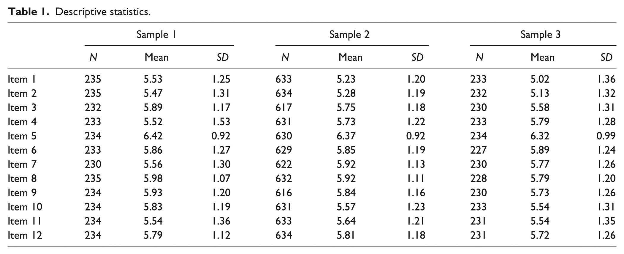
Descriptive Statistics

Table 1 shows number of observations, means, and standard deviations for each item in the three samples. The ICCs for the nesting of patients within therapists in Sample 2 ranged from .06 to .15, showing that most of the variance in the indicators was on the within-therapist level. Thus, the amount of statistical dependency was not alarmingly high. To test the joint significance of variances at the therapist level, we estimated a two-level model with all between-level variances constrained to zero and compared this to a model in which between-level variances were estimated freely. The chi-square difference test was statistically nonsignificant (Δχ² = 16.37, df = 12, p = .17), indicating that estimating therapist level variances did not significantly improve model fit. Because of this, all subsequent models were run as single-level models.

Table 1.

Descriptive statistics.

	Sample 1			Sample 2			Sample 3
	N	Mean	SD	N	Mean	SD	N	Mean	SD
Item 1	235	5.53	1.25	633	5.23	1.20	233	5.02	1.36
Item 2	235	5.47	1.31	634	5.28	1.19	232	5.13	1.32
Item 3	232	5.89	1.17	617	5.75	1.18	230	5.58	1.31
Item 4	233	5.52	1.53	631	5.73	1.22	233	5.79	1.28
Item 5	234	6.42	0.92	630	6.37	0.92	234	6.32	0.99
Item 6	233	5.86	1.27	629	5.85	1.19	227	5.89	1.24
Item 7	230	5.56	1.30	622	5.92	1.13	230	5.77	1.26
Item 8	235	5.98	1.07	632	5.92	1.11	228	5.79	1.20
Item 9	234	5.93	1.20	616	5.84	1.16	230	5.73	1.26
Item 10	234	5.83	1.19	631	5.57	1.23	233	5.54	1.31
Item 11	234	5.54	1.36	633	5.64	1.21	231	5.54	1.35
Item 12	234	5.79	1.12	634	5.81	1.18	231	5.72	1.26

Confirmatory Factor Analyses of WAI-SR

Factor models were first run on all three samples using ML with robust standard errors,² assuming exactly zero cross-loadings and residual correlations, in order to test our first hypothesis that the likelihood ratio chi-square test of exact fit would show significant ill-fit for such a model. As can be seen in Table 2, statistically significant chi-square tests show that exact fit tests failed for all models in all samples (as expected). When reestimating the same models (i.e., models assuming exactly zero cross-loadings and residual correlations) using Bayesian estimation, results were the same (see right-hand side columns of Table 2). This is also expected, since Bayesian estimation with noninformative priors relies only on the data likelihood and should thus yield similar estimates as ML.

Table 2.

Model Fit for Maximum Likelihood and Bayesian Estimation, Assuming Exactly Zero Cross-Loadings and Residual Correlations.

	Maximum likelihood robust					Bayesian
	χ²	df	p	AIC	BIC	χ² 95% CI	PP p	DIC	BIC
Sample 1
One-factor	223.9	54	<.001	7669.9	7794.5	231.5, 295.8	<.001	7670.4	7795.4
Two-factor	108.6	53	<.001	7505.1	7633.2	65.7, 131.6	<.001	7507.0	7634.1
Three-factor	98.5	51	<.001	7494.4	7629.3	55.7, 123.2	<.001	7500.1	7630.6
Sample 2
One-factor	901.2	54	<.001	17962.8	18123.2	1287.3, 1389.2	<.001	17963.0	18123.6
Two-factor	449.8	52	<.001	17233.2	17398.0	610.5, 682.8	<.001	17234.7	17398.4
Three-factor	418.1	51	<.001	17172.8	17346.5	551.6, 627.7	<.001	17178.2	17347.0
Sample 3
One-factor	351.4	54	<.001	7297.2	7421.6	429.3, 509.0	<.001	7297.8	7422.6
Two-factor	206.0	53	<.001	7075.3	7085.9	217.6, 292.9	<.001	7077.1	7204.0
Three-factor	184.5	51	<.001	7038.9	7050.1	184.5, 260.5	<.001	7045.9	7174.9

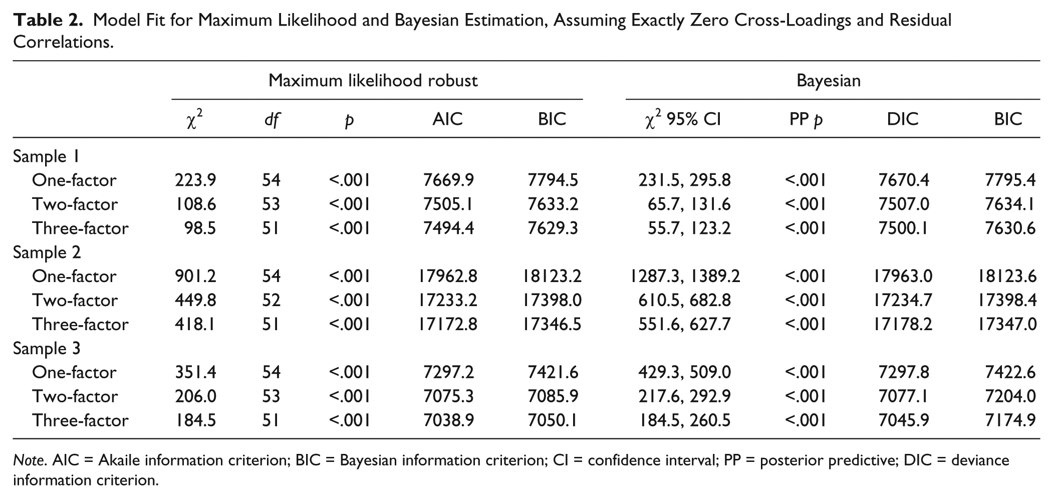
Note. AIC = Akaile information criterion; BIC = Bayesian information criterion; CI = confidence interval; PP = posterior predictive; DIC = deviance information criterion.

Table 3 shows that estimating cross-loadings using zero mean and small variance priors improved model fit somewhat, but these models were still unacceptable in terms of model fit. However, estimating residual correlations using zero mean and small variance priors resulted in excellent model fit in all three samples (i.e., posterior predictive p values very close to .50 and 95% confidence interval symmetrically centered around zero).³

Table 3.

Model Fit Information Using Bayesian Estimation With Informative Priors for Cross-Loadings and Residual Covariances.

	Cross-loadings				Residual covariances
	χ² 95% CI	PP p	DIC	BIC	χ² 95% CI	PP p	DIC	BIC
Sample 1
One-factor					−33.1, 46.4	.37	7468.3	7842.5
Two-factor	47.4, 113.6	<.001	7494.6	7675.9	−29.9, 48.3	.33	7466.1	7854.7
Three-factor	32.1, 102.2	<.001	7484.3	7734.2	−30.1, 49.9	.31	7465.6	7868.1
Sample 2
One-factor					−37.6, 38.6	.51	16616.2	17101.2
Two-factor	491.5, 568.9	<.001	17126.5	17351.3	−36.8, 39.3	.48	16619.3	17109.5
Three-factor	198.6, 293.2	<.001	16837.5	17132.9	−36.4, 39.5	.47	16619.7	17124.6
Sample 3
One-factor					−35.1, 41.6	.42	6860.4	7237.2
Two-factor	140.4, 221.4	<.001	7007.4	7188.1	−34.0, 44.0	.41	6857.5	7247.6
Three-factor	114.7, 209.7	<.001	6995.5	7244.4	−33.1, 45.5	.39	6857.5	7261.3

Note. CI = confidence interval; PP = posterior predictive; DIC = deviance information criterion; BIC = Bayesian information criterion.

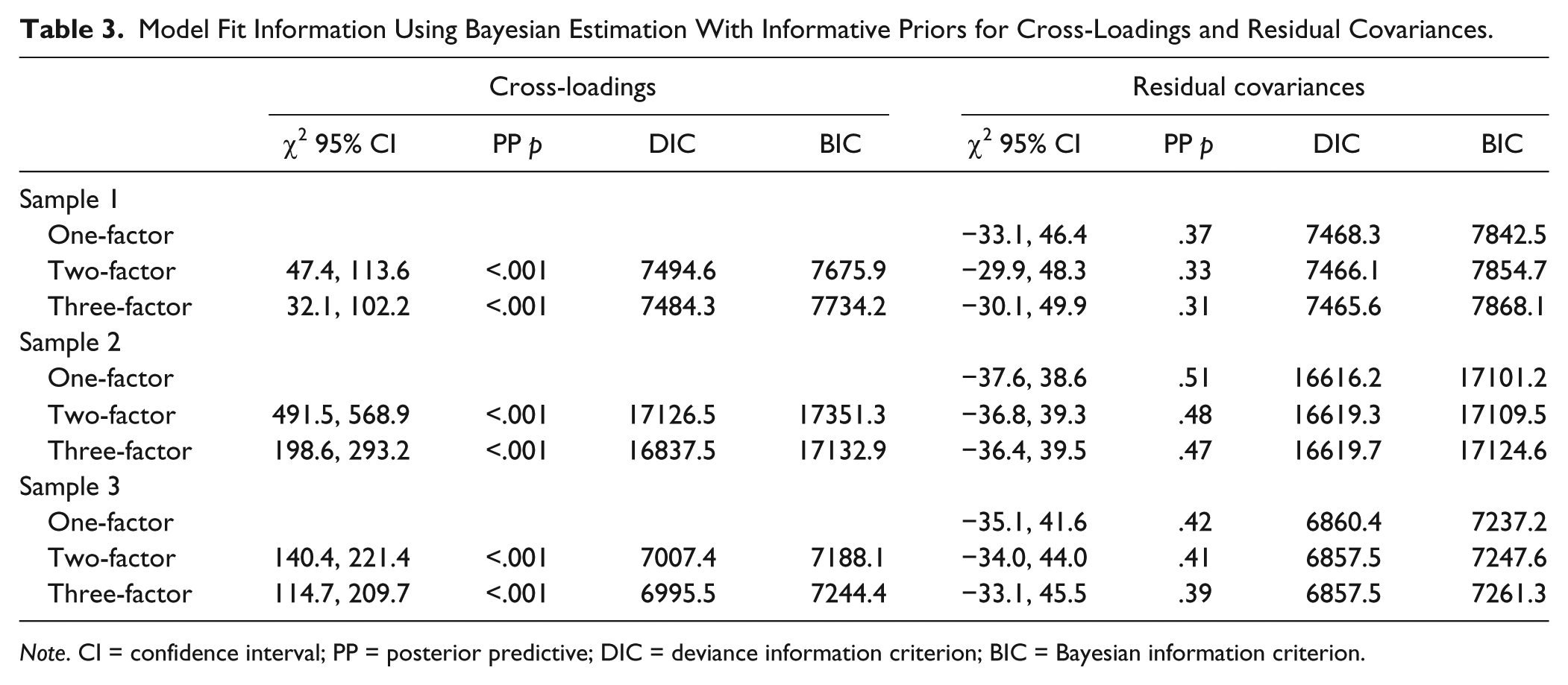
The source of model ill-fit for the ML estimated models thus seemed to be identified in the form of residual correlations between indicators. However, although zero-mean and small variance priors were used for the residual correlations, there is still a chance that some residual correlations are estimated outside the 95% confidence interval specified by the priors. This is especially likely with large samples, because in large samples the posterior distribution will be dominated more by the data than by the prior. If this is the case, the BSEM assumption of residual correlations being small and trivial may be violated. Statistical significance of residual correlations may not be a good indicator of violation of the BSEM assumption for two reasons: (a) with informative priors, standard errors will become smaller due to the additional information in the priors; and (b) in a large sample even trivial correlations may attain statistical significance. Instead, we chose to use a criterion of ±.30 for possibly nontrivial standardized residual correlations.

In Table 4, estimated residual correlations larger than ±.30 for all three models in all three samples are presented. Few residual correlations were the same in all three samples, indicating that some were likely due to chance. This is especially likely since 66 residual correlations were estimated for each of three models in three different samples (summing up to 594 residual correlations). However, there were some that were similar across at least two samples. In all three samples the one-factor model had a number of relatively large residual correlations between items belonging to the Bond factor, indicating that two- or three-factor models may be preferable to the one-factor model. In Sample 1, the two- and three-factor models had only a couple of residual correlations that were slightly above the criterion, indicating that these models both fit the BSEM assumption well. In Sample 2, the two- and three-factor models both had four residual correlations above the criterion, which is also not much considering the number of correlations estimated. Inspecting the content of Items 1 and 2, which showed the largest residual correlation that persisted across all three models in both Swedish samples, showed that both could be interpreted as an evaluation of what has been achieved so far in therapy (Item 1, “As a result of these sessions I am clearer as to how I might be able to change,” and Item 2, “What I am doing in therapy gives me new ways of looking at my problem”), that is, more of achieved outcome than alliance. However, the American participants did not seem to interpret them this way, because the residual correlation between these two items was essentially zero in Sample 1.

Table 4.

Residual Correlations Larger Than ±.30 for One-, Two-, and Three-Factor Solutions Using Bayesian Estimation With Zero Mean, Small Variance Priors for Residual Correlations.

	Sample 1			Sample 2			Sample 3
Items (subscales)	1 Factor	2 Factor	3 Factor	1 Factor	2 Factor	3 Factor	1 Factor	2 Factor	3 Factor
1 and 2 (T-T)				.58	.50	.46	.45	.39	.32
1 and 4 (T-G)								−.31
1 and 5 (T-B)							−.32
1 and 6 (T-G)					−.33			−.38	−.31
1 and 7 (T-B)				−.31			−.40	−.35	−.33
1 and 9 (T-B)							−.41	−.36	−.33
1 and 12 (T-T)			−.33
2 and 6 (T-G)					−.33
2 and 7 (T-B)							−.33
2 and 9 (T-B)							−.33
2 and 12 (T-T)									−.32
3 and 7 (B-B)	.36			.57			.43
3 and 9 (B-B)	.40			.34			.36
3 and 10 (B-T)				−.34
3 and 11 (B-G)				−.37			−.30
3 and 12 (B-T)				−.32
4 and 6 (G-G)							.45	.44	.36
4 and 11 (G-G)						−.31		−.34	−.48
5 and 6 (B-G)					.32
5 and 7 (B-B)							.33
5 and 8 (B-G)		.32	.32
5 and 9 (B-B)	.30						.34
6 and 7 (G-B)								.33
6 and 9 (G-B)								.36	.32
6 and 11 (G-G)									−.40
7 and 9 (B-B)	.37			.43			.45
7 and 11 (B-G)							−.34
10 and 11 (T-G)				.37		.40
10 and 12 (T-T)				.33
11 and 12 (G-T)				.31		.33			.34

Sample 3 showed somewhat more violations of the BSEM assumption. The two-factor model had 9 and the three-factor model 10 residual correlations above the criterion. However, five of these were just slightly above the postulated ±.30 criterion, and involved Items 1 and 2. The Goal scale showed a positive residual correlation between Items 4 and 6, while Item 11 correlated negatively with both Items 4 and 6. Inspecting the content of these items, Items 4 and 6 have comparatively similar wordings in that both explicitly ask for evaluations of the goal aspect of the alliance (Item 4 about agreement on goals and Item 6 about working toward agreed upon goals). Item 11, on the other hand, also asks for evaluation of the goal aspect of the alliance, but without mentioning the word “goal.” Perhaps this wording factor contributed to the slightly elevated residual correlations for this factor.

For model comparisons, we used the models without cross-loadings or residual correlations, because of a concern that cross-loadings and/or residual correlations might muddle comparisons. For example, constraints put on the less complex models might lead to higher residual correlations, with the result that possible misfit of these models would not show up in the model fit tests but in the residual correlations instead (making comparisons much more difficult). Inspection of Table 2 shows that AIC/DIC (Akaile information criterion/deviance information criterion) and BIC (Bayesian information criterion) values consistently favored the three-factor model to the other models.

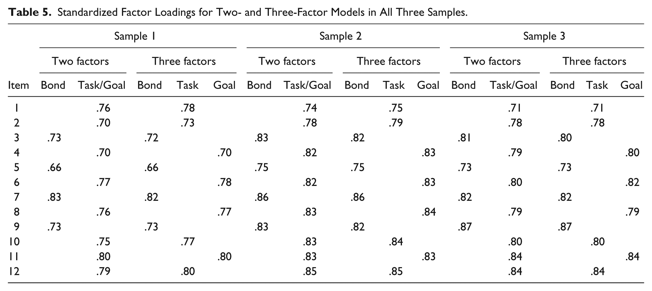
Table 5 shows standardized factor loadings for the two- and three-factor models estimated using zero-mean and small variance priors for residual correlations. Factor loadings were generally strong, with somewhat stronger loadings in the two Swedish samples. In Sample 1 there was one loading below .70 (Item 5 of the Bond scale) and most of the other loadings were between .70 and .80, while in Samples 2 and 3 the loadings ranged between .71 and .87.

Table 5.

Standardized Factor Loadings for Two- and Three-Factor Models in All Three Samples.

	Sample 1					Sample 2					Sample 3
	Two factors		Three factors			Two factors		Three factors			Two factors		Three factors
Item	Bond	Task/Goal	Bond	Task	Goal	Bond	Task/Goal	Bond	Task	Goal	Bond	Task/Goal	Bond	Task	Goal
1		.76		.78			.74		.75			.71		.71
2		.70		.73			.78		.79			.78		.78
3	.73		.72			.83		.82			.81		.80
4		.70			.70		.82			.83		.79			.80
5	.66		.66			.75		.75			.73		.73
6		.77			.78		.82			.83		.80			.82
7	.83		.82			.86		.86			.82		.82
8		.76			.77		.83			.84		.79			.79
9	.73		.73			.83		.82			.87		.87
10		.75		.77			.83		.84			.80		.80
11		.80			.80		.83			.83		.84			.84
12		.79		.80			.85		.85			.84		.84

Previous research has shown that when cross-loadings are assumed to be exactly zero, factor intercorrelations are overestimated (see Marsh, Morin, Parker, & Kaur, 2014). Because of this, we report factor intercorrelations from the models with cross-loadings estimated using zero means and small variance priors. The factor correlations, shown in Table 6, were still generally quite high, particularly the Task–Goal correlation, which was over .90 in Sample 1 and Sample 3 (.93 and .92, respectively), with Sample 2 slightly lower but still quite high (.82). This means that these two factors shared between 67% and 86% variance, indicating that, in general, the scale does not meaningfully differentiate these two constructs. For the two-factor model, factor intercorrelations ranged between .69 in Sample 1 and .80 in Sample 2. Although these factors were also strongly correlated, it may still be statistically meaningful to differentiate them.

Table 6.

Factor Intercorrelations for Two- and Three-Factor Models in All Three Samples^a.

	Sample 1		Sample 2		Sample 3
2 Factors	Task/Goal		Task/Goal		Task/Goal
Bond	.69		.80		.76
3 Factors	Goal	Task	Goal	Task	Goal	Task
Bond	.70	.66	.77	.74	.87	.65
Goal		.93		.82		.92

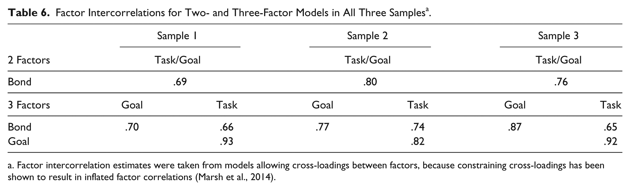
Factor intercorrelation estimates were taken from models allowing cross-loadings between factors, because constraining cross-loadings has been shown to result in inflated factor correlations (Marsh et al., 2014).

Measurement Invariance Analyses Across Samples

It seems from Tables 5 and 6 that there were some differences between the English and Swedish language versions, although the general pattern was the same. To formally test for differences, we performed measurement invariance analyses among the three samples, following the steps suggested by van de Schoot, Lugtig, and Hox (2012). Model fit for the configural, metric, and scalar invariance models is shown in Table 7. For all comparisons, metric invariance held, as indicated by nonsignificant chi-square difference tests and ΔCFI smaller than .01 (Cheung & Rensvold, 2002). When the Swedish and English samples were compared, scalar invariance did not hold, as shown by both significant chi-square difference tests and ΔCFI larger than .01. However, for the comparison between the two Swedish samples, scalar invariance held.

Table 7.

Measurement Invariance Across Samples for the Three-Factor Model Using the Maximum Likelihood Estimator With Robust Standard Errors.

	Sample 1 vs. Sample 2			Sample 1 vs. Sample 3			Sample 2 vs. Sample 3
Model	Δχ² (df)^a	p	CFI	Δχ² (df)^a	p	CFI	Δχ² (df)^a	p	CFI
Configural			.919			.924			.906
Metric	14.3 (9)	.11	.917	5.9 (9)	.75	.924	6.1 (9)	.73	.905
Scalar	94.8 (18)	<.001	.905	81.4 (18)	<.001	.901	24.6 (18)	.14	.901

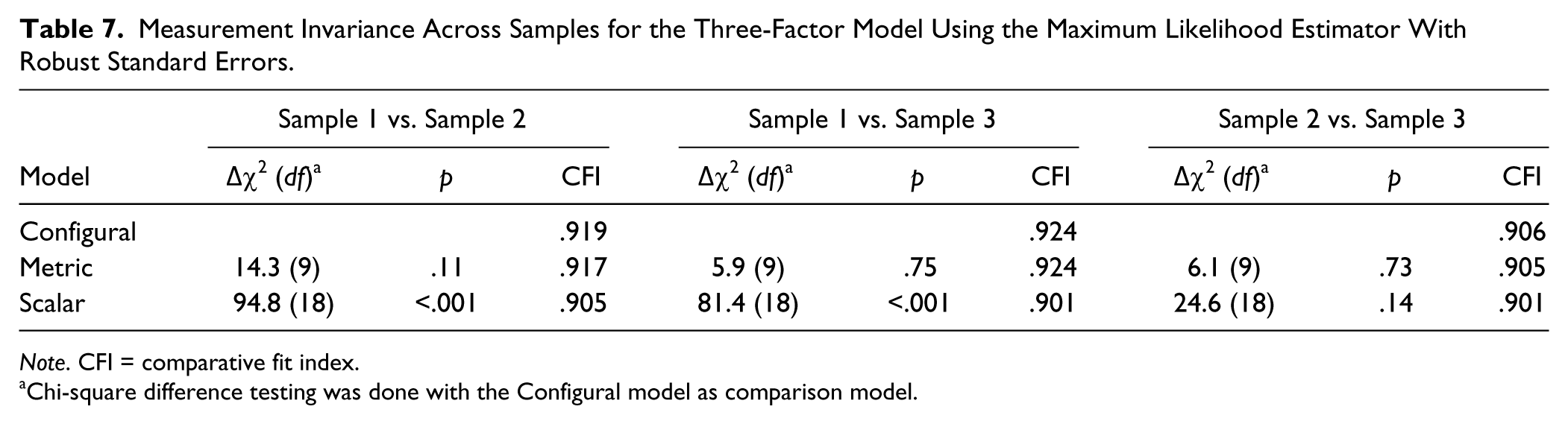
Note. CFI = comparative fit index.

Chi-square difference testing was done with the Configural model as comparison model.

Measurement Invariance Across Treatments

All three samples consisted of mixed treatment populations. Since it is theoretically likely that the working alliance differs between treatment orientations (Bordin, 1979), it is also possible that the factor structure of a working alliance instrument will differ across treatments. Samples 1 and 3, however, were deemed too small to divide into subgroups based on treatment types. In Sample 2, therapists specified therapy type but had the option of marking more than one therapy orientation for each therapy. This option was chosen quite often (34%), indicating that most of the treatments were eclectic. However, we categorized treatments that the therapist had chosen the orientation “psychodynamic” or “relational” as the first choice into a “PDT” group (N = 120); treatments characterized primarily as “behavioral,” “cognitive,” or “cognitive-behavioral” into a “CBT” group (N = 100); and the rest were categorized as an “Other” group (N = 415). Results of measurement invariance tests are shown in Table 8. As Table 8 shows, the metric model failed the chi-square difference test, but passed the ΔCFI criterion (ΔCFI = .005). The scalar model just passed the chi-square difference test (compared to the configural model) and passed the ΔCFI criterion (ΔCFI = −.007). Testing the difference between PDT and CBT only yielded similar results.

Table 8.

Measurement Invariance Analyses Across Treatment Types^a for the Three-Factor Model Using the Maximum Likelihood Estimator With Robust Standard Errors.

	Sample 1			Sample 2			Sample 3
Model	Δχ² (df)^b	p	CFI	Δχ² (df)^a	p	CFI	Δχ² (df)^a	p	CFI
Configural						.902
Metric				36.6 (18)	.006	.897
Scalar				50.8 (36)	.052	.895

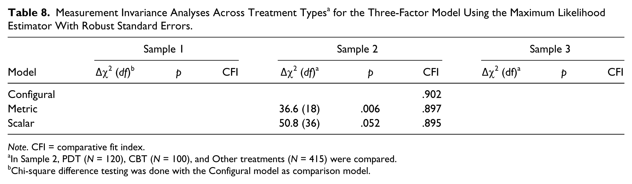
Note. CFI = comparative fit index.

In Sample 2, PDT (N = 120), CBT (N = 100), and Other treatments (N = 415) were compared.

Chi-square difference testing was done with the Configural model as comparison model.

Discussion

This study evaluated the factor structure of the patient version of the WAI-SR using three relatively large clinical samples. The results from the BSEM analyses showed that one-, two-, and three-factor models all fit data well when small residual correlations between indicators were allowed. A major advantage of Bayesian estimation with informative priors is that this method allows estimation of models that are not identified when ML estimation is used (neither the model with all cross-loadings nor the one with all residual correlations estimated would be identified with ML).

However, when estimating all possible residual correlations, the question arises as to how many or how large residual correlations that can be allowed before the model structure should be questioned? Because this method is relatively new, there are as yet no rules of thumb for this (B. O. Muthén, personal communication, November 20, 2013). We used a criterion of ±.30 for a standardized residual correlation to be considered “potentially nontrivial.” Using this criterion, inspection of residual correlations for the two- and three-factor models showed that the one-factor model had elevated residual correlations for the items belonging to the Bond factor, thus indicating that this factor should be estimated separately. Except for this, there were very few residual correlations above the criterion in Samples 2 and 3, and there were none that were the same across all three samples, indicating that most of the other residual correlations above the criterion were due to chance. We therefore conclude that the BSEM assumption that small and trivial residual correlations were responsible for misfit of models assuming exactly zero residual correlations held. This is an improvement from previous confirmatory factor analyses of the WAI, because the misspecification indicated by significant likelihood ratio chi-square tests in these analyses was identified. This is not to say that diagnosing misfit cannot be done using ML, just that this to our knowledge has not been done previously for the WAI. However, the BSEM approach has an advantage compared with the standard approach of using modification indices to diagnose misfit, in that modification indices inform about model improvement when a single parameter is freed while the BSEM method informs about improvement when all parameters are freed at the same time. The result is that when using modification indices, the researcher may need to respecify the model several times before finding a well-fitting model, a practice that increases the risk for capitalizing on chance. With BSEM usually only one respecification needs to be done (see also B. O. Muthén and Asparouhov, 2012, for more details).

The residual correlation between Items 1 and 2, which was relatively high in all models in the two Swedish samples, may be due to the fact that both items ask about the effects of the therapy on the patients’ experience of the goals and tasks of therapy rather than focusing specifically on the patients’ current experience of the alliance. Because one criticism of alliance research has been that the alliance–outcome correlation could be influenced by prior outcome, it is unfortunate if some items can be interpreted as asking for prior outcome (even if one might expect that alliance itself would grow and develop over the course of therapy). Perhaps these items should be deleted or changed in future versions of the WAI. Some of the other residual correlations can be understood as resulting from similar item content, for example, Items 4 and 6 belonging to the Goal factor, which had relatively high residual correlations in all models in Sample 3.

Another improvement from previous CFAs of the WAI is that the statistical dependency created by nesting of patients within therapists has previously been ignored, thus assuming that the factor structure is not affected by this level of nesting. Our analysis in Sample 2 showed that model fit did not improve significantly when testing a model that separates variance due to therapists from variance due to patients, thus confirming that this level could in fact be ignored without biased estimates.

No previous study has to our knowledge investigated measurement invariance for the WAI. The measurement invariance analyses between groups showed that the factor structure was stable across Swedish and English versions of the scale. The more stringent scalar invariance did not hold across languages/cultures, indicating that data from the Swedish translation should not be combined with data from the English version in the same analysis. The fact that scalar invariance did hold between the two Swedish samples indicates that these samples can in fact be combined and compared even using composite means, which is a very stringent test of the stability of a scale (Steinmetz, 2013). In addition, measurement invariance seemed to hold across treatment orientations, although this was only possible to test in one of the three samples.

The intercorrelation between the Task and Goal factors in the three-factor model was high across all three samples (especially Samples 1 and 3), indicating that in general these factors cannot be differentiated. Still, meaningful differences between these scales are sometimes found in substantive research (e.g., Hoffart, Øktedalen, Langkaas, & Wampold, 2013). Because of this it may be premature to conclude that the Task and Goal factors should be combined into one. Future research may focus on finding subsamples, perhaps of patient groups or of treatment orientations, in which the Task and Goal factors are more clearly separable. Until such groups are found, however, we have to conclude that a two-factor structure in which the Task and Goal factors are collapsed into one is psychometrically more defensible than a three-factor structure.

An interesting question for future research is if all 12 items of the WAI-SR are needed for reliably measuring the working alliance, especially if a two-factor model is the one that will be used? Although the WAI-SR is already a brief version of the original 36-item WAI (Horvath & Greenberg, 1989), its internal consistency (coefficient alpha) was .95 in both Swedish samples and .92 in the American sample. This is very high, and may indicate item redundancy. Even subscales had very high internal consistencies; for the Bond scale alpha was .91 in both Swedish samples and .86 in the American sample, while the combined Task/Goal scale had alphas of .92 to .94. Because recent research has started to use session-to-session measurement of the working alliance (Falkenström et al., 2013; Hoffart et al., 2013; Tasca & Lampard, 2012), an “ultra-brief” alliance measure would be desirable in order not to unnecessarily burden patients.

Limitations of the present study include the fact that BSEM is a new method and the interpretation of correlated residuals is not yet well studied. More generally, an issue for future research to explore is the extent to which Bayesian estimation with informative priors can be used to estimate models that are not identified using ML. Although the Bayesian estimation methods seem to have great potential for extending possibilities for model estimation, informative priors need to be used with great care so that the researcher’s prior beliefs does not bias estimation results. As with any statistical method, assumptions need to be clearly stated so that readers can evaluate their tenability. Another limitation is the fact that we could only test multilevel factor analysis on one of the three samples, since we did not have information about which patients were treated by the same therapist in the other two samples. Future studies should test measurement invariance across other grouping variables such as gender or diagnosis. In addition, since the WAI is increasingly being used in longitudinal research as a time-varying predictor, longitudinal measurement invariance will be important to evaluate.

Footnotes

Appendix

Working Alliance Inventory–Short form Revised (Hatcher & Gillaspy, 2006)

1. As a result of these sessions I am clearer as to how I might be able to change.

2. What I am doing in therapy gives me new ways of looking at my problem.

3. I believe ___ likes me.

4. ___ and I collaborate on setting goals for my therapy.

5. ___ and I respect each other.

6. ___ and I are working towards mutually agreed upon goals.

7. I feel that ___ appreciates me.

8. _____ and I agree on what is important for me to work on.

9. I feel _____ cares about me even when I do things that he/she does not approve of.

10. I feel that the things I do in therapy will help me to accomplish the changes that I want.

11. _____ and I have established a good understanding of the kind of changes that would be good for me.

12. I believe the way we are working with my problem is correct.

Declaration of Conflicting Interests

The authors declared no potential conflicts of interest with respect to the research, authorship, and/or publication of this article.

Funding

The authors disclosed receipt of the following financial support for the research, authorship, and/or publication of this article: This research was supported by a post-doctoral grant (2013-0203) to Fredrik Falkenström by the Swedish Research Council for Health, Working Life and Wellfare. The other authors received no financial support for the research, authorship, and/or publication of this article.

Notes

References

Alexander

L. B.

Luborsky

(1986). The Penn Helping Alliance Scales. In Greenberg

L. S.

Pinsof

W. M.

(Eds.), The psychotherapeutic process: A research handbook (pp. 325-366). New York, NY: Guilford Press.

Andrusyna

T. P.

Tang

T. Z.

Derubeis

R. J.

Luborsky

(2001). The factor structure of the Working Alliance Inventory in cognitive-behavioral therapy. Journal of Psychotherapy Practice and Research, 10, 173-178.

Asparouhov

Muthén

B. O.

(2010). Bayesian analysis using Mplus: technical implementation. Technical appendix. Los Angeles: Muthén & Muthén. Retrieved from www.statmodel.com

Baldwin

S. A.

Wampold

B. E.

Imel

Z. E.

(2007). Untangling the alliance-outcome correlation: Exploring the relative importance of therapist and patient variability in the alliance. Journal of Consulting and Clinical Psychology, 75, 842-852. doi:10.1037/0022-006X.75.6.842

Bentler

P. M.

Bonett

D. G.

(1980). Significance tests and goodness of fit in the analysis of covariance structures. Psychological Bulletin, 88, 588-606. doi:10.1037/0033-2909.88.3.588

Bordin

E. S.

(1979). The generalizability of the psychoanalytic concept of the working alliance. Psychotherapy: Theory, Research & Practice, 16, 252-260.

Busseri

M. A.

Tyler

J. D.

(2003). Interchangeability of the Working Alliance Inventory and Working Alliance Inventory, Short Form. Psychological Assessment, 15, 193-197. doi:10.1037/1040-3590.15.2.193

Cheung

G. W.

Rensvold

R. B.

(2002). Evaluating goodness-of-fit indexes for testing measurement invariance. Structural Equation Modeling: A Multidisciplinary Journal, 9, 233-255. doi:10.1207/S15328007SEM0902_5

Crits-Christoph

Gallop

Temes

C. M.

Woody

Ball

S. A.

Martino

Carroll

K. M.

(2009). The alliance in motivational enhancement therapy and counseling as usual for substance use problems. Journal of Consulting and Clinical Psychology, 77, 1125-1135. doi:10.1037/a0017045

10.

Crits-Christoph

Gibbons

M. B. C.

Hamilton

Ring-Kurtz

Gallop

(2011). The dependability of alliance assessments: The alliance-outcome correlation is larger than you might think. Journal of Consulting and Clinical Psychology, 79, 267-278. doi:10.1037/a0023668

11.

DeRubeis

R. J.

Brotman

M. A.

Gibbons

C. J.

(2005). A conceptual and methodological analysis of the nonspecifics argument. Clinical Psychology: Science and Practice, 12, 174-183. doi:10.1093/clipsy/bpi022

12.

Falkenström

Granström

Holmqvist

(2013). Therapeutic alliance predicts symptomatic improvement session by session. Journal of Counseling Psychology, 60, 317-328. doi:10.1037/a0032258

13.

Falkenström

Granström

Holmqvist

(2014). Working alliance predicts psychotherapy outcome even while controlling for prior symptom improvement. Psychotherapy Research, 24, 146-159. doi:10.1080/10503307.2013.847985

14.

Flückiger

Del Re

A. C.

Wampold

B. E.

Symonds

Horvath

A. O.

(2012). How central is the alliance in psychotherapy? A multilevel longitudinal meta-analysis. Journal of Counseling Psychology, 59, 10-17. doi:10.1037/a0025749

15.

Gaston

(1991). Reliability and criterion-related validity of the California Psychotherapy Alliance Scales–Patient Version. Psychological Assessment: A Journal of Consulting and Clinical Psychology, 3, 68-74. doi:10.1037/1040-3590.3.1.68

16.

Gelman

Carlin

J. B.

Stern

H. S.

Dunson

D. B.

Vehtari

Rubin

D. B.

(2014). Bayesian data analysis (3rd ed.). Boca Raton, FL: CRC Press.

17.

Hatcher

R. L.

Barends

A. W.

(1996). Patients’ view of the alliance in psychotherapy: Exploratory factor analysis of three alliance measures. Journal of Consulting and Clinical Psychology, 64, 1326-1336. doi:10.1037/0022-006x.64.6.1326

18.

Hatcher

R. L.

Gillaspy

J. A.

(2006). Development and validation of a revised short version of the Working Alliance Inventory. Psychotherapy Research, 16, 12-25. doi:10.1080/10503300500352500

19.

Hayduk

Cummings

Boadu

Pazderka-Robinson

Boulianne

(2007). Testing! testing! one, two, three—Testing the theory in structural equation models! Personality and Individual Differences, 42, 841-850. doi:10.1016/j.paid.2006.10.001

20.

Hoffart

Øktedalen

Langkaas

T. F.

Wampold

B. E.

(2013). Alliance and outcome in varying imagery procedures for PTSD: A study of within-person processes. Journal of Counseling Psychology, 60, 471-482. doi:10.1037/a0033604

21.

Holmqvist

Ström

Foldemo

(2014). The effects of psychological treatment in primary care in Sweden—A practice-based study. Nordic Journal of Psychiatry, 68, 204-212. doi:10.3109/08039488.2013.797023

22.

Horvath

A. O.

(2000). The therapeutic relationship: From transference to alliance. Journal of Clinical Psychology, 56, 163-173. doi:10.1002/(sici)1097-4679(200002)56:2<163::aid-jclp3>3.0.co;2-d

23.

Horvath

A. O.

Del Re

Fluckiger

Symonds

(2011). Alliance in individual psychotherapy. Psychotherapy, 48, 9-16. doi:10.1037/a0022186

24.

Horvath

A. O.

Greenberg

L. S.

(1989). Development and validation of the Working Alliance Inventory. Journal of Counseling Psychology, 36, 223-233.

25.

Horvath

A. O.

Symonds

B. D.

(1991). Relation between working alliance and outcome in psychotherapy: A meta-analysis. Journal of Counseling Psychology, 38, 139-149. doi:10.1037/0022-0167.38.2.139

26.

Kaplan

Depaoli

(2012). Bayesian structural equation modeling. In Hoyle

R. H.

(Ed.), Handbook of structural equations modeling (pp. 650-673). New York, NY: Guilford Press.

27.

Little

(2013). Longitudinal structural equations modeling. New York, NY: Guilford Press.

28.

Marsh

H. W.

Morin

A. J. S.

Parker

P. D.

Kaur

(2014, November). Exploratory structural equation modeling: An integration of the best features of exploratory and confirmatory factor analysis. Annual Review of Clinical Psychology, 10, 85-110. doi:10.1146/annurev-clinpsy-032813-153700

29.

McIntosh

C. N.

(2007). Rethinking fit assessment in structural equation modelling: A commentary and elaboration on Barrett (2007). Personality and Individual Differences, 42, 859-867. doi:10.1016/j.paid.2006.09.020

30.

Munder

Wilmers

Leonhart

Linster

H. W.

Barth

(2010). Working Alliance Inventory-Short Revised (WAI-SR): Psychometric properties in outpatients and inpatients. Clinical Psychology & Psychotherapy, 17, 231-239.

31.

Muthén

B. O.

(1991). Multilevel factor analysis of class and student achievement components. Journal of Educational Measurement, 28, 338-354.

32.

Muthén

B. O.

Asparouhov

(2012). Bayesian structural equation modeling: A more flexible representation of substantive theory. Psychological Methods, 17, 313-335. doi:10.1037/a0026802

33.

Muthén

L. K.

Muthén

B. O.

(1998-2012). Mplus user’s guide (7th ed.). Los Angeles, CA: Muthén & Muthén.

34.

O’Malley

S. S.

Suh

C. S.

Strupp

H. H.

(1983). The Vanderbilt Psychotherapy Process Scale: A report on the scale development and a process-outcome study. Journal of Consulting and Clinical Psychology, 51, 581-586. doi:10.1037/0022-006x.51.4.581

35.

Reise

S. P.

Ventura

Nuechterlein

K. H.

Kim

K. H.

(2005). An illustration of multilevel factor analysis. Journal of Personality Assessment, 84, 126-136.

36.

Rigdon

E. E.

(2012). Rethinking partial least squares path modeling: In praise of simple methods. Long Range Planning, 45, 341-358. doi:10.1016/j.lrp.2012.09.010

37.

Roesch

S. C.

Aldridge

A. A.

Stocking

S. N.

Villodas

Leung

Bartley

C. E.

Black

L. J.

(2010). Multilevel factor analysis and structural equation modeling of daily diary coping data: Modeling trait and state variation. Multivariate Behavioral Research, 45, 767-789. doi:10.1080/00273171.2010.519276

38.

Steinmetz

(2013). Analyzing observed composite differences across groups: Is partial measurement invariance enough? Methodology: European Journal of Research Methods for the Behavioral and Social Sciences, 9(1), 1-12. doi:10.1027/1614-2241/a000049

39.

Tasca

G. A.

Lampard

A. M.

(2012). Reciprocal influence of alliance to the group and outcome in day treatment for eating disorders. Journal of Counseling Psychology, 59, 507-517. doi:10.1037/a0029947

40.

Tracey

T. J.

Kokotovic

A. M.

(1989). Factor structure of the Working Alliance Inventory. Psychological Assessment: A Journal of Consulting and Clinical Psychology, 1, 207-210. doi:10.1037/1040-3590.1.3.207

41.

Van de Schoot

Lugtig

Hox

(2012). A checklist for testing measurement invariance. European Journal of Developmental Psychology, 9, 486-492. doi:10.1080/17405-629.2012.686740

42.

Vandenberg

R. J.

Lance

C. E.

(2000). A review and synthesis of the measurement invariance literature: Suggestions, practices, and recommendations for organizational research. Organizational Research Methods, 3(1), 4–69. doi:10.1177/109442810031002

43.

Webb

C. A.

DeRubeis

R. J.

Amsterdam

J. D.

Shelton

R. C.

Hollon

S. D.

Dimidjian

(2011). Two aspects of the therapeutic alliance: Differential relations with depressive symptom change. Journal of Consulting and Clinical Psychology, 79, 279-283. doi:10.1037/a0023252

44.

Zilcha-Mano

Dinger

McCarthy

K. S.

Barber

J. P.

(2014). Does alliance predict symptoms throughout treatment, or is it the other way around? Journal of Consulting and Clinical Psychology, 82(6), 931-935 doi:10.1037/a0035141

45.

Zuroff

D. C.

Kelly

A. C.

Leybman

M. J.

Blatt

S. J.

Wampold

B. E.

(2014). Between-therapist and within-therapist differences in the quality of the therapeutic relationship: Effects on maladjustment and self-critical perfectionism. Journal of Clinical Psychology, 66, 681-697. doi:10.1002/jclp.20683

46.

Zyphur

M. J.

Oswald

F. L.

(2015). Bayesian estimation and inference: A user’s guide. Journal of Management, 41(2), 390-420 doi:10.1177/0149206313501200

Confirmatory Factor Analysis of the Patient Version of the Working Alliance Inventory–Short Form Revised

Abstract

Keywords

Method

Participants

Sample 1

Sample 2

Sample 3

Measures

Working Alliance Inventory–Short Form Revised (Hatcher & Gillaspy, 2006)

Statistical Analyses

Bayesian Structural Equations Modeling

Measurement Invariance

Multilevel Data Structure

Results

Descriptive Statistics

Confirmatory Factor Analyses of WAI-SR

Measurement Invariance Analyses Across Samples

Measurement Invariance Across Treatments

Discussion

Footnotes

Appendix

Declaration of Conflicting Interests

Funding

Notes

References