Modeling BAS Dysregulation in Bipolar Disorder

Abstract

Time series analysis is a technique that can be used to analyze the data from a single subject and has great potential to investigate clinically relevant processes like affect regulation. This article uses time series models to investigate the assumed dysregulation of affect that is associated with bipolar disorder. By formulating a number of alternative models that capture different kinds of theoretically predicted dysregulation, and by comparing these in both bipolar patients and controls, we aim to illustrate the heuristic potential this method of analysis has for clinical psychology. We argue that, not only can time series analysis elucidate specific maladaptive dynamics associated with psychopathology, it may also be clinically applied in symptom monitoring and the evaluation of therapeutic interventions.

Keywords

time series analysis regime-switching dynamic system intensive longitudinal data

The clinician knows he is dealing with process. He cannot help but remain unimpressed with statistical procedures and results which are applied to observations made at comparatively isolated points in time, and which do not tell him something of what has been happening along the way.

—Jack B. Chassan, (1959, p. 397)

Many psychiatric disorders are defined in terms of increased or decreased variability in affect, behavior, and cognition, and/or particular patterns in these fluctuations. For instance, obsessive compulsive disorder is characterized by recurrent thoughts and behaviors that have to be carried out in order to control stress and anxiety; posttraumatic stress disorder is characterized by alternating episodes of avoidance and intrusions; major depressive disorder is characterized by decreased and flattened positive affect and a lack of energy; panic disorder is characterized by episodes of disproportional fear; and certain eating disorders are characterized by episodes of binging and/or starving. Such dynamic signatures only show up over time, such that intensive longitudinal measurements are mandatory if we want to investigate them.

Although the plea for a person-oriented approach based on intensive longitudinal data has repeatedly been made over the past decades (cf. Cattell, 1966; Chassan, 1959; Molenaar, 2004; Nesselroade, 2002), it remained a rather exotic endeavor for a long time. However, as the result of technological developments such as pagers, actigraphs, and smartphones, obtaining intensive longitudinal data has now become within reach of mainstream psychology, and the methodology toolbox has been extended with novel techniques such as ambulatory assessment, electronic diaries, ecological momentary assessments and experience sampling method (Conner, Tennen, Fleeson, & Feldman Barrett, 2009; Trull & Ebner-Priemer, 2014). These developments open up new possibilities in the study of all kinds of psychological phenomena, but they are especially promising in the area of clinical psychology and psychopathology (Conner & Feldman Barrett, 2012; Trull & Ebner-Priemer, 2013). For instance, the network perspective that has been introduced recently as an alternative framework for understanding vulnerability to psychopathology (cf. Borsboom & Cramer, 2013; Wichers et al., 2009), merges very naturally with person-oriented research based on intensive longitudinal data: The combination allows for the investigation of individual networks of symptoms, which indicate how a particular person may start to spiral downward as a result of a relatively minor change, whereas another person remains resilient even under rather extreme circumstances (Bringmann et al., 2013; van der Krieke et al., 2015). Related to this, there is a rapidly growing field referred to as mHealth or eHealth, which uses technological devices, not only to monitor physical and mental health, but also as a way to intervene in maladaptive processes through providing feedback (cf., Kramer et al., 2014; Mohr, Schueller, Montague, Burns, & Rashidi, 2014; Strecher, 2007).

A psychiatric disorder that may benefit from a more process-oriented approach in particular, is bipolar disorder (BD). Hallmark features of this disorder are major fluctuations in affect and activity, as well as marked changes in perception and cognition. A deeper understanding of the particular dynamical signature of BD—the nature of these fluctuations and what triggers them—would help predict and hopefully even prevent some of the adverse effects this disease has. To date, however, the number of studies using intensive longitudinal data to focus on BD is seriously lagging behind similar studies that focus on depression and borderline personality disorder (cf. aan het Rot, Hogenelst, & Schroevers, 2012; Ebner-Priemer & Trull, 2009), although there are a few (e.g., Bauer et al., 2004; Bauer et al., 2006). While the reason for this difference is unclear, we believe that the unknown nature of BD fluctuations—which are therefore difficult to actually model—is playing a key role here.

To tackle this problem, we set out to show how time series analysis may be used to explore the fluctuations associated with BD. Time series analysis is a technique that is frequently used in other disciplines, such as econometrics, meteorology, physics, and seismography, and is based on modeling the sequential dependencies that are present in time series data (i.e., large numbers of repeated measures from a single case). Because time series analysis is in essence an N = 1 technique, it is a truly idiographic approach that results in the description of the pattern of fluctuations for a particular individual. Such a focus may prove especially valuable when the interest is in monitoring a patient’s symptoms and optimizing treatment. Additionally, however, we may compare the results from multiple patients and see how they differ from nonpatients, in order to distill the dynamic signature that is associated with a particular process: This could form a first, inductive step in exploring this new research area. Hence, whereas we focus on BD here, we expect that this approach—if properly adjusted—will also prove valuable in the study of other psychological processes.

We begin by briefly discussing the background of BD and the hypothesized role that the behavioral approach system (also known as behavioral activation system, BAS) is assumed to play in the characteristic fluctuations associated with BD. Next, we present a number of statistical models that can generate diverse patterns of fluctuations, and relate these to diverse ideas about the kind of dysregulation BD patients suffer. These models can be used to analyze N = 1 data, making it an appropriate tool for studying (dys)regulation per individual. Subsequently, we present empirical data from 3 BD patients and 11 healthy controls, which we first analyze individually and subsequently compare with each other. We end with a discussion in which we point out future directions for this line of research.

BAS Dysregulation in BD

The BAS dysregulation theory postulates that BD patients have an overly sensitive BAS that is hyperreactive to BAS-relevant cues (cf. Depeu & Iacono, 1989; Hofmann & Meyer, 2006; Johnson, Edge, Holmes, & Carver, 2012; Urošević, Abramson, Harmon-Jones, & Alloy, 2008). On one hand, activation of the BAS is associated with expected reinforcement and reward, as well as increased positive affect and activity, which in extreme cases may result in mania. On the other hand, inactivation of the BAS is associated with anticipating a lack of reward, energy loss, decreased positive affect, and ultimately depression. The BAS dysregulation theory holds that BD patients are characterized by more extreme changes in BAS activation than healthy controls. However, while a variety of studies have found support for this theory (e.g., Alloy & Abramson, 2008; Depeu et al., 1981; Harmon-Jones & Allen, 1997; Hofmann & Meyer, 2006; Holzwarth & Meyer, 2006; Johnson et al., 2012; Knowles et al., 2007; Lovejoy & Steuerwald, 1995; Myin-Germeys et al., 2003), the actual nature of dysregulation remains unknown (cf. Gruber, Kogan, Mennin, & Murray, 2013).

Some have suggested that BAS dysregulation associated with BD consists of a lack of regulatory strength of the BAS, such that return to the individual’s baseline or set point after the system has been (de)activated takes much longer in BD patients than in healthy people (Holzwarth & Meyer, 2006; Wright, Lam, & Brown, 2008). This corresponds to the description of BD as a rollercoaster ride (e.g., Urošević et al., 2008), in which the patient experiences (more or less) smooth transitions from one extreme to another, while covering a much wider range on activation and affective dimensions than healthy people.

Alternatively, BAS dysregulation may result in BD symptoms once the BAS activity trespasses a certain threshold (Holzwarth & Meyer, 2006). In this line of thinking, BD may be conceived of as a dynamic system that is characterized by two attractors, one associated with mania, and the other associated with depression: When the system moves into the proximity of one such attractor, it is drawn into this state and thus the system tends to remain there unless an external force disrupts the system and makes it switch to the other attractor (cf. van der Maas & Molenaar, 1992). This view corresponds with the suggestion by Urošević et al. (2008) about the key role of appraisal in BD. These authors state that if a patient is in the manic state, he or she appraises more events as relevant with respect to BAS activation (i.e., as opportunities for goal or reward attainment), he or she creates more BAS activating-events, and he or she assumes more efficacy in reaching goals or rewards. In contrast, when in the depressed state the patient appraises more events as BAS deactivating (i.e., as a failure or loss), and also appraises his/her efficacy as lower, which results in increased feelings of hopelessness. Hence, the patient’s appraisal (of events as well as of personal efficacy) is, on one hand, affected by the state he or she is in, while on the other hand it also helps shape and maintain the state that he or she is in. This implies that once the patient has entered a certain state, he or she is likely to stay in this state, which corresponds to the idea of attractors.

Next we propose a number of time series models that mimic these two distinct forms of dysregulation.

Time Series Analysis to Model BAS Dysregulation

We propose five mathematical–statistical models that can be used to describe day-to-day fluctuations in mood. These models all have in common that today’s mood (i.e., y_t) is a function of yesterday’s mood (i.e., f(y_t _{− 1})) and that there is an unpredictable part (i.e., u_t), which is referred to as the residual, innovation, perturbation or random shock. The latter is a collection of all the relevant factors—internal and external, psychological and physiological—that affect the daily affective process. The models differ from one another in the way that yesterday’s mood influences today’s mood: While some of these models are consistent with the idea of a slow return to baseline, others are characterized by switches between distinct states or regimes. Below we describe each of these models and how they are related to the two proposed forms of dysregulation, and in Figure 1 we have included graphical representations of these models, along with a brief description. Furthermore, Figure 1S in the supplementary material (available at http://asm.sagepub.com/content/by/supplemental-data), sequences of different instances of these models are given, to illustrate the diverse behaviors that can stem from them. After presenting the five models, we briefly outline our expectations with respect to these models in the context of BD.

Figure 1.

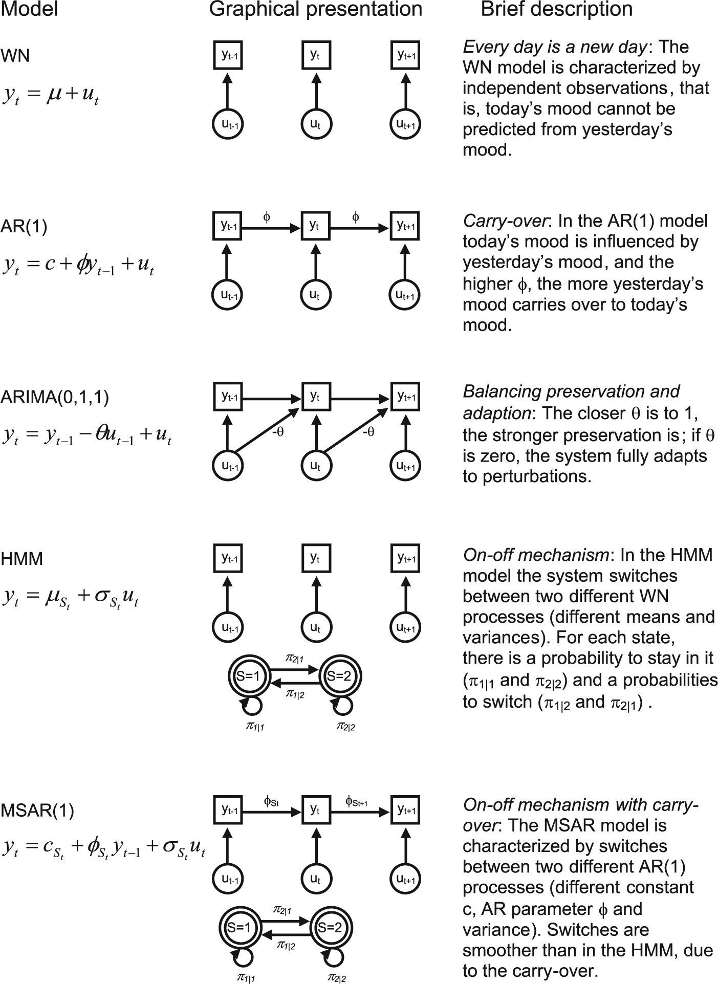
Five time series models: equations, graphical representation, and description.

Model 1: Every Day Is a New Day

The first model we consider is a white noise (WN) model, which is a rather simple model in which today’s mood actually does not depend on yesterday’s mood. People who have an affective system that can be described as a WN process can be said to experience every day as a new day. Because of this lack of “memory,” this parsimonious model can be interpreted as the most stable possible form of a dynamic system in the current context.

Model 2: Slow-Return-to-Baseline due to Carryover

The second model is a first-order autoregressive (AR(1)) process (Hamilton, 1994), which we use to model slow-return-to-baseline. In this model, today’s mood is predicted from yesterday’s mood, using the AR coefficient φ (see Figure 1). This coefficient is referred to as the inertia, as the closer it is to one, the more reluctant a person is to change from one occasion to the next. This also means that perturbations that occurred in the past and that influenced the person’s mood are carried over to consecutive days, and continue to have an influence on mood the following days, although the intensity diminishes as time passes. If the AR coefficient is zero, this process reduces to a WN process as discussed above, in which there is no carryover from one day to the next.

Model 3: Slow-Return-to-Baseline due to Lack of Preservation

The ARIMA(0,1,1) model is a special case of the more general autoregressive integrated moving average model (e.g., Hamilton, 1994), and balances two oppositional forces: adaption and preservation (Fortes, Delignières, & Ninot, 2004). While adaption implies that a perturbation to the system has a lasting effect, in contrast, preservation is a controlling mechanism, which manifests itself as a resistance to change away from one’s baseline. The moving-average parameter θ in the ARIMA(0,1,1) model forms the balance between adaption and preservation (see also Figure 1S in the supplementary material): If θ is close to 1, the system is dominated by preservation, which implies a quick return to baseline; in contrast, when θ is closer to 0 this is characteristic of a system that is dominated by adaption, which implies a slow return to baseline resulting in roller coaster behavior.

Model 4: On–Off Mechanism

The fourth model we consider is a hidden Markov (HM) model that includes two latent states or regimes: At every measurement occasion, the person is in one of these regimes. These regimes are characterized by different means (for instance, a manic state is associated with higher levels of positive affect than a depressed state), but may also differ with respect to the variances; for instance, there may be more variability in the manic state than in the depressed state (e.g., Depeu et al., 1981). The switching from one state to the other depends on the transition probabilities, which are denoted as π_j|i, which represents the probability of switching to regime j if one is in regime i (where j = 1, 2 and i = 1, 2). In general, we may assume that an individual tends to remain in the same state for at least several days, such that π_1|1 > π_2|1 and π_2|2 > π_1|2.

Model 5: On–Off Mechanism With Carryover

The final model we consider is the MSAR (Markov switching autoregressive) model (Hamilton, 1989; Kim & Nelson, 1999), which can be thought of as a combination of the HM model and the AR model discussed previously: While the HM model is characterized by white noise sequences within each state (meaning that within a state there are no dependencies over time), the MSAR model is characterized by AR processes in each state; as a result of this carryover, the switches from one state to the other are less abrupt in the MSAR model than in the HM model discussed above. This also implies that events that influenced affect yesterday have an indirect influence on today’s affect, regardless of whether one stays in the same regime or switches to another regime.

This model has been suggested before as a way to describe regime-switching associated with BD, and has been compared with other regime-switching models (i.e., threshold AR models) by Hamaker, Grasman, and Kamphuis (2010). They concluded that the MSAR model provided a better description of affect fluctuations in a BD patient, than the other regime-switching models that were considered.

Expectations

It is important to note that we are not assuming that healthy affect regulation implies a WN model, while the other models necessarily imply maladaptive forms of affect regulation. For instance, we believe it is natural to have some carryover from yesterday’s mood to today’s mood (cf. Suls, Green, & Hillis, 1998), although this is not necessarily the case; thus far, multilevel autoregressive models have reported average autoregressive parameters for daily affective measurements in the range of about .2 to .3 (Jongerling, Laurenceau, & Hamaker, 2015; Kuppens, Allen, & Sheeber, 2010; Suls et al., 1998), although other psychological phenomena and measurement frequencies may result in lower and even negative values (e.g. Rovine & Walls, 2006). It has been noted that if the carryover effect becomes very large, this implies that the system is quite unstable and may wander off both in the positive or the negative direction away from its equilibrium (Kuppens et al., 2010; van de Leemput et al., 2014). Hence, whether or not a specific system is maladaptive might be a quantitative rather than a qualitative matter. Therefore, it is not only important to determine which model provides the best description of the data and whether this is different for BD patients and controls (which would represent a qualitative difference), but it is also important to look at the specific parameter values of the selected model and how BD patients and controls differ from each other with respect to these (which would form a quantitative difference).

Having said this, we expect that the WN model (Model 1) will not be appropriate for describing the affect regulation in BD patients, although it may be suitable for (some) healthy persons. With respect to the other models, we mainly expect quantitative differences: (a) for the AR(1) model (Model 2), we expect BD patients to have higher inertias φ than healthy controls; (b) for the ARIMA(0,1,1) model (Model 3), we expect the balance parameter θ to be closer to zero in BD patents than in healthy controls; and (c) in the regime-switching models (Models 4 and 5) we expect states that can be clearly identified as mania and depression in BD patients, whereas regime differences in healthy controls may be of a different nature.¹

Method

Participants

The data we use here originate from two separate daily diary studies, and were gathered independently by the first and last author in 2009 and 2007 respectively (see the online supporting material for details). In total we consider three BD patients diagnosed with rapid cycling BD (which we refer to as P1 to P3), and eleven healthy controls (which we refer to as C1 to C11) in the current study.

Instruments

Participants in both studies completed the Positive Affect and Negative Affect Schedule (PANAS; Watson & Tellegen, 1985), at a daily basis for approximately 90 days. The PANAS results in a positive affect (PA) score and a negative affect (NA) score. Theoretically, PA is associated with the BAS, the hypothesized neurological system that controls motivation and goal directed behavior, such that BAS activation is associated with higher levels of PA, while BAS deactivation is associated with lower PA (Carver & White, 1994; Holzwarth & Meyer, 2006; Watson, Wiese, Vaidya, & Tellegen, 1999). In contrast, NA has been related to the Behavioral Inhibition System (BIS), which is assumed to regulate punishment-avoidance through withdrawal behaviors and passive avoidance (Carver & White, 1994; Watson et al., 1999), that is, an activated BIS is associated with high NA, while a deactivated BIS is associated with low NA (Holzwarth & Meyer, 2006). Hence, theoretically mania and depression are predominantly related to PA and the BAS, whereas NA and the BIS are assumed to be connected to anxiety and phobias. Although BIS sensitivity is not assumed to play a particular role in BD, aggression and hostility—which are part of the NA scale—have been associated with BAS activity also (cf. Beaver, Lawrence, Passamonti, & Calder, 2008). Therefore, and to allow for a full dimensional approach to affect in both BD patients and controls, we decided to focus on both PA and NA in our analyses.

Analysis

We analyzed the data of each individual separately using bivariate (i.e., vector) extensions of the models discussed before, such that PA and NA could be modeled simultaneously. In all five models we included correlations between the residuals of PA and NA, which implies that the unpredictable parts of both PA and NA may have some common sources (i.e., relevant external or internal stimuli that day). In the AR model and the MSAR model the bivariate extension meant that besides the AR parameters from PA yesterday to PA today, and from NA yesterday to NA today, there were also cross-lagged regression coefficients from PA yesterday to NA today and from NA yesterday to PA today (Hamaker et al., 2010; Hamilton, 1994). For details on the software we used, see the online supporting material.

Results

In Figure 2, the sequences of all 3 patients and 11 controls for PA and NA are depicted, showing that the BD patients are characterized by a much larger variation in PA than the controls (see also the reported variances in Table 1S in the supplementary material available at http://asm.sagepub.com/content/by/supplemental-data). This is in agreement with the BAS dysregulation hypothesis and confirms earlier results (Depeu et al., 1981; Hofmann & Meyer, 2006; Lovejoy & Steuerwald, 1995). However, what we are particularly interested in here is whether patients and controls differ with respect to their underlying dynamics, that is, the patterns of temporal dependencies that govern the fluctuations in their affect. Based on the sequences in Figure 2, this is not easy to determine. Therefore, we begin by discussing the comparison of the five models of interest for each participant. Subsequently, we focus on the best fitting model per person and compare the parameter estimates across individuals.

Figure 2.

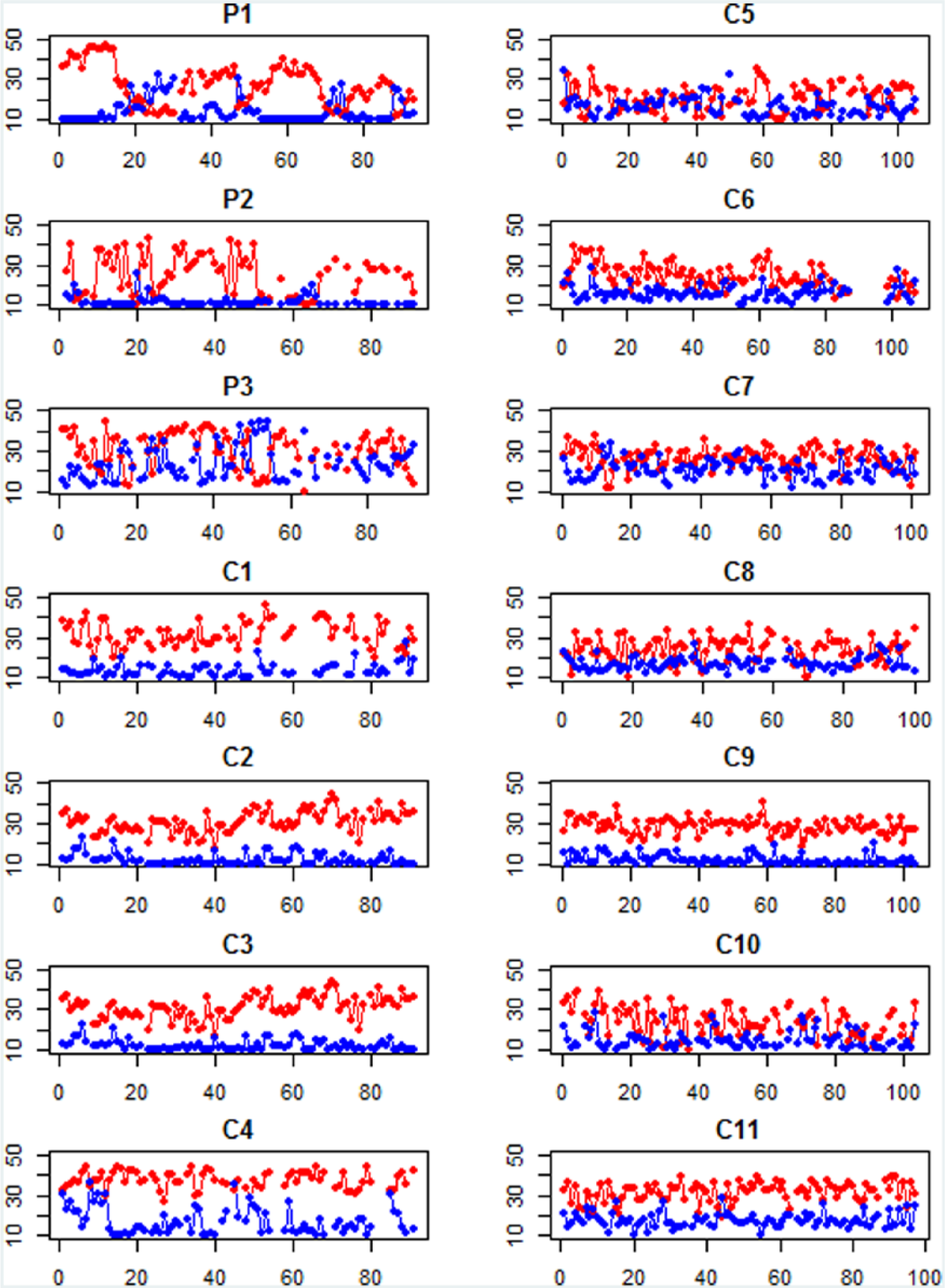
Daily positive affect (PA; in red) and negative affect (NA; in blue) recordings for 3 bipolar disorder (BD) patients (P1 to P3) and 11 controls (C1 to C11).

Model Comparison

To compare the five models, we make use of model weights (Burnham & Anderson, 2002), which are presented in Table 1: These model weights add up to 1, and are interpreted as a measure of the relative support in the data for each of the models that is considered. Model weights are based on the Bayesian information criterion (BIC; Schwarz, 1978), which consists of −2 times the log likelihood of the model plus a penalty for model complexity (i.e., the number of parameters that is estimated in the model multiplied by the log of the number of observations). While the BIC can be used to compare nested and nonnested models (with smaller values pointing to better models), the difference between two (or more) BICs are less intuitive than the model weights used here (for the BICs, see Table 2S in the supplementary material available at http://asm.sagepub.com/content/by/supplemental-data).

Table 1.

Model Weights Based on the BIC for the Five Time Series Models.

	WN	VAR(1)	VARIMA (0,1,1)	HMM	MSAR
P1	<.001	<.001	<.001	<.001	1.000
P2	<.001	<.001	<.001	1.000	<.001
P3	<.001	<.001	1.000	<.001	<.001
C1	.001	<.000	.001	.997	<.001
C2	<.001	.001	.267	.727	.005
C3	.007	<.001	.993	—	—
C4	<.001	<.001	<.001	1.000	<.001
C5	<.001	.999	<.001	.001	<.001
C6	<.001	<.001	1.000	<.001	<.001
C7	.499	.499	.002	<.001	<.001
C8	.002	<.001	.998	<.001	<.001
C9	<.001	<.001	<.001	1.000	<.001
C10	<.001	<.001	<.001	1.000	<.001
C11	.982	.001	.011	.007	<.001

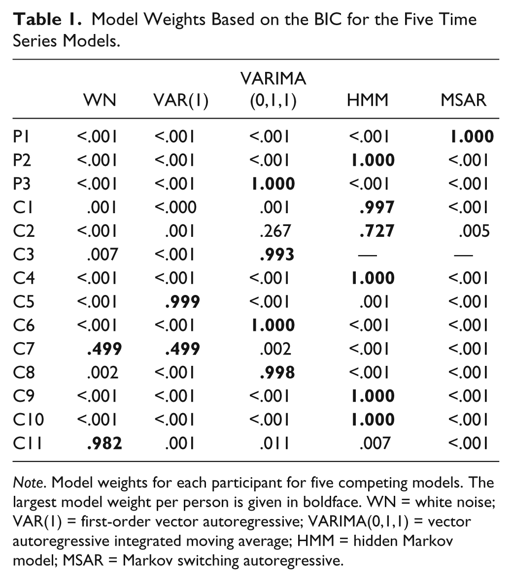
Note. Model weights for each participant for five competing models. The largest model weight per person is given in boldface. WN = white noise; VAR(1) = first-order vector autoregressive; VARIMA(0,1,1) = vector autoregressive integrated moving average; HMM = hidden Markov model; MSAR = Markov switching autoregressive.

The results in Table 1 show that for P1 and P2, a regime-switching model is selected, which is also the most appropriate model for 5 of the 11 controls (i.e., C1, C2, C4, C9, and C10). In contrast, the data of P3 are best described with a VARIMA(0,1,1) model, which also proved the most appropriate model for 3 of the 11 controls (i.e., C3, C6, and C8). Finally, for the remaining three controls, one was best described by a WN model (C11), the second was best described by a VAR(1) model (C5), while for the third, the WN model and the VAR(1) were equally appropriate (C7).

Clearly, based on the current sample size it is not possible to draw definite conclusions, but the current results seem to suggest that the differences in the affective regulatory mechanisms of BD patients and controls are not of a primarily qualitative nature. That is, while the WN model and VAR(1) model are only selected for controls, both the patients and many of the controls were best described by either the VARIMA(0,1,1) model or the regime-switching models. To obtain more insight in the possible quantitative differences in these cases, we take a closer look at the parameter estimates for these selected models.

Quantitative Comparison for the VARIMA(0,1,1) model

As indicated earlier, the ARIMA(0,1,1) model is characterized by the parameter θ, which balances the tendency to preserve (when θ is close to 1) and adapt (when θ is closer to 0). Figure 3 contains the θ estimates for PA and NA for P3 and the three controls that were best described using this model. It shows that the BD patient is characterized by much lower θ parameters that the controls, which means that it takes this patient longer to return to baseline and restore equilibrium than the controls. This is in agreement with our expectation regarding quantitative differences, implying a slower-return-to-baseline in the patient. Note however that this is true for both PA and NA, which suggests either a general dysregulation (both BAS- and BIS-related), or that the BAS-related component in NA plays an important role in its dynamics (see Figure 1S in the supplementary material, for examples of different ARIMA(0,1,1) behavior).

Figure 3.

Theta estimates with standard errors for patient 3 (P3), and three controls (C3, C6, and C8). Dark bars are for positive affect (PA), and light bars are for negative affect (NA).

Quantitative Comparison for the Regime-Switching Models

With regard to the switching models, we were specifically interested in the means of PA and NA in each regime: These are the values toward which the person’s affect is being pulled and which can thus be interpreted as the attractors of the system. We were interested in whether one of the regimes reflects a manic state, while the other reflects a depressive state.

The HM model was selected for one patient (P1) and five controls (C1, C2, C4, C9, and C10), while the MSAR model was selected for one patient (P2). In Figure 4 we have included the differences in means between the two regimes for both PA and NA separately. Most notable is that the two BD patients are characterized by large mean differences in PA between the two regimes, while none of the controls is characterized by substantial differences in PA. This implies that switches between the two regimes in patients is characterized by substantial changes in PA (and for P1 also in NA), whereas changes in regimes in the controls is associated with changes in NA, but not (or only to a very minor degree) in PA. This result can be interpreted as evidence for the BAS dysregulation theory, given the theoretical link between the BAS and PA: It seems that regime-switching in BD patients is associated with large changes in PA (and thus BAS activation), whereas regime switches in healthy controls is associated with marked changes in NA (and thus BIS activation).

Figure 4.

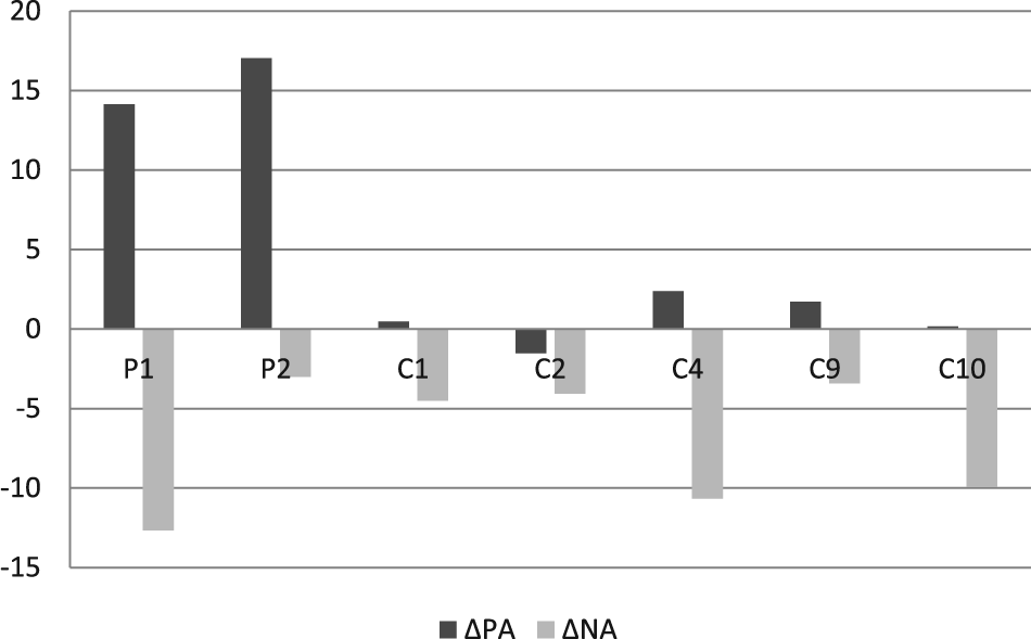
Mean positive affect (PA) and negative affect (NA) difference across two regimes for two patients (P1 and P2), and five controls (C1, C2, C4, C9, and C10).

Based on the probabilities of switching from one regime to the other, we determined that the overall probability to be in regime 1 (which is characterized by high PA and low NA) was .81 for P1 and .75 for P2. For the controls, the overall probability to be in regime 1 (characterized by low NA), was .48 for C1, .32 for C2, .36 for C4, .64 for C9, and .17 for C10.

Discussion

Before summarizing the main substantive findings of the present study, we want to stress that the data we used in the current paper are clearly not ideal: They were gathered through two separate studies and the small number of participants (i.e., 3 BD patients and 11 controls) warrant against generalizing the results to the populations to which these participants belong. Nevertheless, the current study sheds a first light on the affective dynamics associated with BD, and on the differences between BD patients and controls, and it thus illustrated how the endeavor to study process dynamics may take shape.

Our initial research question here was whether BAS dysregulation associated with BD is best understood as a slow-return-to-baseline (as modeled by an AR(1) model or an ARIMA(0,1,1) model), or as a system that is characterized by two attractors that result from the BAS being switched on or off (as modeled with a regime-switching model). Since the best models for the three BD patients came from both categories of time series models, we cannot draw any (preliminary) conclusions about the actual nature of BAS dysregulation.

An additional research question was whether there are qualitative and/or quantitative differences in the patterns of affect fluctuations between BD patients and healthy controls. The selected models indicate that differences between patients and controls are to some extent qualitative: For instance, the WN and AR(1) processes were not descriptive of affect fluctuations in BD patients, but are appropriate for over one third of the controls. Additionally, the differences are to some extent quantitative: For instance, the balance parameter in the ARIMA (0,1,1) model is closer to preservation in controls than in the BD patient, and the states in BD patients show marked differences in PA, while controls show very little changes in PA across states. More generally, we can conclude that the difference in affect regulation between BD patients and controls is not just in the amount of variability, but also in the dynamics. This suggests that—as was already theorized by for instance Holzwarth and Meyer (2006)—BD is more than simply experiencing a wider range of affective responses: The latter would imply that the variance is larger in BD patients than in controls, but not that there are qualitative or quantitative differences in the dynamics themselves, as we were able to detect here.

From a methodological perspective, this article demonstrates how time series models can be used to obtain a deeper understanding of the nature of affective fluctuations associated with a particular mental disorder, and how this may differ from healthy affective fluctuations. The approach taken in the current article is only a first, exploratory step, showing that substantive theories can be converted into particular aspects of statistical models, which can then be fitted and compared. A subsequent step could consist of obtaining more detailed insight in the dynamics of a particular individual by determining how diverse time-varying factors influence the process. For instance, we could extend the time series models considered here such that the parameters that govern the dynamics (i.e., the balance parameter θ in the ARIMA(0,1,1) model, or the switching probabilities π_1|2 and π_2|1 in the regime-switching models) can change over time as a function of sleep quality or interpersonal stress. Once such an idiographic pattern has been established for a particular patient, this may serve as a monitoring tool that generates warnings for the patient and his/her practitioner, when there is an increased risk for the onset of a manic episode for instance, and additionally may even suggest interventions (e.g., more rest, relaxation exercises). As such, this approach could form a valuable contribute to the increased need for more person-tailored treatments in mental health, and it fits well with current developments for gathering intensive longitudinal data from individual patients using new technologies (e.g., Boyce, 2011).

Another direction that could be taken is to try to establish nomothetic insights based on the current idiographic approach. Roughly speaking, there are two possible routes to this goal. In the bottom-up approach, one would perform idiographic analysis such as illustrated here, but with much larger samples, possibly classified according to subtypes and comorbidity. While it is unlikely that individuals within a particular group are all characterized by the exact same model, one hopefully finds meaningful regularities in the way people from diverse groups differ from each other with respect to particular dynamical features, and this would thus give an indication of the dynamic signature associated with different disorders and subtypes. In the top-down approach, on the other hand, one decides beforehand on a particular time series model, and uses this as the level 1 model in a multilevel extension. While this approach implies we have to choose a single model for everybody, thus excluding the possibility of qualitative differences between people, the advantage is that it makes comparisons between individuals straightforward, which explains why this approach is become rather popular at the moment (see Bringmann et al., 2013 for an example).

Both the N = 1 time series approach as well as the multilevel extension of the time series approach could be of interest when the aim is to investigate the effectiveness of certain treatments for mental diseases such as BD, which are characterized by particular dynamic patterns: If a treatment is successful in establishing change, this should be apparent from changes in the structure of patients’ affective dynamics. Since BD is primarily a disease of the affect and energy fluctuations and their regulations, comparing means before and after treatment (as is typically done in treatment studies), is not necessarily the best way to study the effectiveness of a treatment. The approach taken here implies that treatment effects may also take on other forms, such as being less reactive to ordinary negative events that take place in one’s life (cf. Wichers et al., 2009).

The techniques and models used here are by no means exhaustive, and there are many other time series based approaches that researchers may wish to consider, both for single subject and multiple subject data (cf. Hamaker, Ceulemans, Grasman, & Tuerlinckx, 2015; Hamaker & Dolan, 2009). Four additional comments are in place here. First, there are diverse measures that can be used for model selection; in the current study we used the BIC, but actually a thorough simulation study is required to decide which measure is most successful in selecting the correct model, and this may depend on the models one wishes to use. Second, most time series models are based on the assumption that the observations are made at equal intervals, which makes these models ideal for daily diary data, but less suitable for data obtained through experience sampling method; the latter are typically characterized by varying intervals between the measurements. This mismatch may be circumvented by adding missing observations such that the intervals become approximately equal, but how successful such an approach is, should again be investigated in a simulation study. Third, it is at this point unclear how many time points are needed; there is some rule of thumb that at least 50 occasions are needed for N = 1 time series analysis, but as the models grow more complex (e.g., multivariate, or through regime switching), this is most likely not enough. Again, simulations could provide more insight and could be used as the basis for alternative guidelines. Note that such guidelines are also likely to differ depending on whether a (replicated) time series approach is taken, or a multilevel approach is used. Fourth and finally, to make these alternative ways for analyzing intensive longitudinal data accessible to mainstream psychology, we need more—and more user-friendly—software that allow for the estimation and comparison of diverse time series models or multilevel extensions of these.

In conclusion, new technology has made gathering intensive longitudinal data a lot easier and ensures higher quality of such data than previously used methods (e.g., paper-and-pencil diary studies); as a result the number of studies based on intensive longitudinal data is increasing rapidly, and with this development comes a need for more advanced modeling techniques that help us to gain insight in the particular dynamical features of psychological processes. While our empirical application is clearly limited in its selection and number of participants, variables, and frequency of measurements—such that great caution should be exercised in drawing substantive conclusions from this demonstration—we hope that it nevertheless triggers the readers’ curiosity about this alternative way to study mental disorders and psychological processes, and that it provides a useful illustration of how substantive theories can be translated into model features, such that they can be estimated and compared statistically. In so doing, we hope to contribute to the important shift from studying outcomes of processes to studying the actual processes themselves, a regime change that Chassan (1959) was already calling for more than half a century ago.

Footnotes

Declaration of Conflicting Interests

The author(s) declared no potential conflicts of interest with respect to the research, authorship, and/or publication of this article.

Funding

The author(s) disclosed receipt of the following financial support for the research, authorship, and/or publication of this article: This study was supported by the Netherlands Organization for Scientific Research (NWO; VIDI grant 452-10-007, awarded to E. L. Hamaker).

Notes

References

aan het Rot

Hogenelst

Schroevers

R. S.

(2012). Mood disorders in everyday life: A systematic review of experience sampling and ecological momentary assessment studies. Clinical Psychological Review, 32, 510-523.

Alloy

L. B.

Abramson

L. Y.

(2008). The role of the behavioral approach system (BAS) in bipolar spectrum disorders. Current Directions in Psychological Science, 19, 189-194.

Bauer

Grof

Gyulai

Rasgon

Glenn

Whybrow

P. C.

(2004). Using technology to improve longitudinal studies: Self-reporting with ChronoRecord in bipolar disorder. Bipolar Disorders, 6, 67-74.

Bauer

Grof

Rasgon

Bschor

Glenn

Whybrow

P. C.

(2006). Temporal relation between sleep and mood in patients with bipolar disorder. Bipolar Disorders, 8, 160-167.

Beaver

J. D.

Lawrence

A. D.

Passamonti

Calder

A. J.

(2008). Appetitive motivation predicts the neural response to facial signals of aggression. Journal of Neuroscience, 12, 2719-2725.

Borsboom

Cramer

A. O. J.

(2013). Network analysis: An integrative approach to the structure of psychopathology. Annual Review of Clinical Psychology, 9, 91-121.

Boyce

(2011). The Lancet technology: August, 2011. Lancet, 378, 475.

Bringmann

L. F.

Vissers

Wichers

Geschwind

Kuppens

Peeters

. . . Tuerlinckx

(2013). A network approach to psychopathology: New insights into clinical longitudinal data. PLoS ONE, 8, e60188.

Burnham

K. P.

Anderson

D. R.

(2002). Model selection and multimodel inference: A practical information-theoretic approach (2nd ed.). New York, NY: Springer.

10.

Carver

C. S.

White

T. L.

(1994). Behavioral inhibition, behavioral activation, and affective responses to impending reward and punishment: The BIS/BAS scales. Journal of Personality and Social Psychology, 67, 319-333.

11.

Cattell

R. B.

(1966). Patterns of change: Measurement in relation to state-dimension, trait change, lability, and process concepts. In Cattell

R. B.

(Ed.), Handbook of multivariate experimental psychology (pp. 355-402). Chicago, IL: Rand McNally.

12.

Chassan

J. B.

(1959). On the development of clinical statistical systems for psychiatry. Biometrics, 15, 396-404.

13.

Conner

T. S.

Feldman Barrett

(2012). Trends in ambulatory self-report: The role of momentary experience in psychosomatic medicine. Psychosomatic Medicine, 74, 327-337.

14.

Conner

T. S.

Tennen

Fleeson

Feldman Barrett

(2009). Experience Sampling Methods: A modern idiographic approach to personality research. Social and Personality Psychology Compass, 3, 292-313. doi:10.1111/j.1751-9004.2009.00170.x

15.

Depeu

R. A.

Iacono

W. G.

(1989). Neurobehavioral aspects of affective disorders. Annual Review of Psychology, 40, 457-492.

16.

Depeu

R. A.

Slater

J. F.

Wolfstetter-Kausch

Klein

Goplerud

Farr

(1981). A behavioral paradigm for identifying persons at risk for bipolar depression disorder: A conceptual framework and five validation studies. Journal of Abnormal Psychology, 90, 381-437.

17.

Ebner-Priemer

U. W.

Trull

T. J.

(2009). Ecological momentary assessment of mood disorders and mood regulation. Psychological Assessment, 21, 463-475.

18.

Fortes

Delignières

Ninot

(2004). The dynamics of self-esteem and physical self: Between preservation and adaption. Quality and Quantity, 38, 735-751.

19.

Gruber

Kogan

Mennin

Murray

(2013). Real-world emotion? An experience-sampling approach to emotion experience and regulation in bipolar I disorder. Journal of Abnormal Psychology, 122, 971-983.

20.

Hamaker

E. L.

Ceulemans

Grasman

R. P. P. P.

Tuerlinckx

(2015). Modeling affect dynamics: State of the art and future challenges. Emotion Review, 7, 316-322.

21.

Hamaker

E. L.

Dolan

C. V.

(2009). Idiographic data analysis: Quantitative methods—from simple to advanced. In Valsiner

Molenaar

P. C. M.

Lyra

M. C. D. P.

Chaudhary

(Eds.). Dynamic process methodology in the social and developmental sciences (pp. 191-216). New York, NY: Springer-Verlag.

22.

Hamaker

E. L.

Grasman

R. P. P. P.

Kamphuis

J. H.

(2010). Regime-switching models to study psychological processes. In Molenaar

P. C. M.

Newell

(Eds.). Individual pathways of change (pp. 155-168). Washington, DC: American Psychological Association.

23.

Hamilton

J. D.

(1989). A new approach to the economic analysis of nonstationary time series and the business cycle. Econometrica, 57, 357-384.

24.

Hamilton

J. D.

(1994). Time series analysis. Princeton, NJ: Princeton University Press.

25.

Harmon-Jones

Allen

J. J. B.

(1997). Behavioral activation sensitivity and resting frontal EEG asymmetry: Covariation of putative indicators related to risk for mood disorders. Journal of Abnormal Psychology, 106, 159-163.

26.

Hofmann

B. U.

Meyer

Th. D.

(2006). Mood fluctuations in people putatively at risk for bipolar disorder. British Journal of Clinical Psychology, 45, 105-110.

27.

Holzwarth

Meyer

Th. D.

(2006). The dysregulation of the “Behavioral Activation System”: An independent dimension. Personality and Individual Differences, 41, 319-328.

28.

Johnson

S. L.

Edge

M. D.

Holmes

M. K.

Carver

C. S.

(2012). The behavioral activation system and mania. Annual Review of Clinical Psychology, 8, 243-267.

29.

Jongerling

Laurenceau

J.-P.

Hamaker

E. L.

(2015). A multilevel AR(1) model: Allowing for inter-individual differences in trait-scores, inertia, and innovation variance. Multivariate Behavioral Research, 50, 334-349.

30.

Kim

C.-J.

Nelson

C. R.

(1999). State-space models with regime switching: Classical and Gibbs-sampling approaches with applications. Cambridge: MIT Press.

31.

Knowles

Tai

Jones

S. H.

Highfield

Morriss

Bentall

R. P.

(2007). Stability of self-esteem in bipolar disorder: Comparison among remitted bipolar patients, remitted unipolar patients and healthy controls. Bipolar Disorders, 9, 490-495.

32.

Kramer

Simons

C. J.

Hartmann

J. A.

Menne-Lothmann

Viechtbauer

Peeters

. . . Wichers

(2014). A therapeutic application of the experience sampling method in the treatment of depression: A randomized controlled trial. World Psychiatry, 13, 68-77.

33.

Kuppens

Allen

N. B.

Sheeber

L. B.

(2010). Emotional inertia and psychological maladjustment. Psychological Science, 21, 984-991.

34.

Lovejoy

M. C.

Steuerwald

B. J.

(1995). Subsyndromal unipolar and bipolar disorder: Comparisons on positive and negative affect. Journal of Abnormal Psychology, 104, 381-384.

35.

Mohr

D. C.

Schueller

S. M.

Montague

Burns

M. N.

Rashidi

(2014). The behavioral intervention technology model: An integrated conceptual and technological framework for eHealth and mHealth interventions. Journal of Medical Internet Research, 16(6), e146.

36.

Molenaar

P. M. C.

(2004). A manifesto on psychology as idiographic science: Bringing the person back into scientific psychology, this time forever. Measurement, 2, 201-218.

37.

Myin-Germeys

Peeters

Havermans

Nicolsons

N. A.

deVries

M. W.

Delespaul

van Os

(2003). Emotional reactivity to daily life stress in psychosis and affective disorder: an experience sampling study. Acta Psychiatrica Scandinavica, 107, 124-131.

38.

Nesselroade

J. R.

(2002). Elaborating the differential in differential psychology. Multivariate Behavioral Research, 37, 543-561.

39.

Rovine

M. J.

Walls

T. A.

(2006). Multilevel autoregressive modeling of interindividual differences in the stability of a process. In Walls

T. A.

Schafer

J. L.

(Eds.), Models for intensive longitudinal data (pp. 124-147). Oxford, England: Oxford University Press.

40.

Schwarz

(1978). Estimating the dimension of a model. Annals of Statistics, 6, 461-464.

41.

Strecher

(2007). Internet methods for delivering behavioral and health-related interventions (eHealth). Annual Review of Clinical Psychology, 3, 53-76.

42.

Suls

Green

Hillis

(1998). Emotional reactivity to everyday problems, affective inertia, and neuroticism. Personality and Social Psychology Bulletin, 24, 127-136.

43.

Trull

T. J.

Ebner-Priemer

(2013). Ambulatory assessment. Annual Review of Clinical Psychology, 9, 151-176.

44.

Trull

T. J.

Ebner-Priemer

(2014). The role of ambulatory assessment in psychological science. Current Directions in Psychological Science, 23, 466-470.

45.

Urošević

Abramson

L. Y.

Harmon-Jones

Alloy

L. B.

(2008). Dysregulation of the behavioral approach system (BAS) in bipolar spectrum disorders: Review of theory and evidence. Clinical Psychological Review, 28, 1188-1205.

46.

van de Leemput

I. A.

Wichers

Cramer

A. O. J.

Borsboom

Tuerlinckx

Kuppens

. . . Scheffer

(2014). Critical slowing down as early warning for the onset and termination of depression. Proceedings of the National Academy of Sciences of the United States of America, 111, 87-92. doi:10.1073/pnas.1312114110

47.

van der Krieke

Jeronimus

B. F.

Blaauw

F. J.

Wanders

R. B.

Emerencia

A. C.

Schenk

H. M.

. . . de Jonge

(2015). HowNutsAreTheDutch (HoeGekIsNL): A crowdsourcing study of mental symptoms and strengths. International Journal of Methods in Psychiatric Research. Advance online publication. doi:10.1002/mpr.1495

48.

van der Maas

H. L. J.

Molenaar

P. C. M.

(1992). Stagewise cognitive development: An application of catastrophe theory. Psychological Review, 99, 395-417.

49.

Watson

Tellegen

(1985). Toward a consensual structure of mood. Psychological Bulletin, 98, 219-235.

50.

Watson

Wiese

Vaidya

Tellegen

(1999). The two general activation systems of affect: Structural findings, evolutionary considerations, and psychobiological evidence. Journal of Personality and Social Psychology, 76, 820-838.

51.

Wichers

M. C.

Barge-Schaapveld

D. Q. C. M.

Nicholson

N. A.

Peeters

de Vries

Mengelers

van Os

(2009). Reduced stress-sensitivity or increased reward experience: The psychological mechanism of response to antidepressant medication. Neuropsychopharmacology, 34, 923-931.

52.

Wright

K. A.

Lam

Brown

R. G.

(2008). Dysregulation of the behavioral activation system in remitted bipolar I disorder. Journal of Abnormal Psychology, 117, 838-848.