Using the De Jong Gierveld Loneliness Scale With Early Adolescents: Factor Structure,Reliability,Stability,and External Validity

Abstract

The present investigation is the first examination of the factor structures, reliability, external validity, longitudinal invariance, and stability of the De Jong Gierveld Loneliness Scale (DJGLS), as used with early adolescents. It is based on a two-wave, large, representative sample of Polish primary school pupils. The results demonstrate that the model most reflective of the factor structure of the DJGLS is the bifactor model, which assumes the occurrence of one, highly reliable, general factor (overall sense of loneliness) and two, relatively irrelevant, subfactors. Essential unidimensionality (the general factor accounting for three fourth of the common variance) suggest that the interpretation of the subfactors over and above the general factor is inappropriate. The longitudinal confirmatory factor analysis indicated that the bifactor structure of the DJGLS is invariant over time. Correlations with self-rated loneliness, sociometric acceptance/rejection, social self-efficacy, identification with class group, family structure, and gender provide support for the validity of the DJGLS. This implies that it could be used as a measure of loneliness in adolescence, which does not involve references to the school context, making it possible to conduct studies that go beyond school period and compare the intensity of the feeling of loneliness in that group with other age groups.

Keywords

loneliness psychometric properties factor structure bifactor longitudinal invariance external validation

The Concept of Loneliness

Loneliness is an unpleasant and stressful feeling, an emotional state charged with sadness and pain, originating in a deficit between the expected and actual or perceived state of an individual’s social relationships in which the need for intimacy is not met (Asher & Weeks, 2013; de Jong Gierveld, 1987; Parkhurst & Hopmeyer-Gorman, 1999; Peplau, 1982). Let us note that brief periods of situational loneliness may fulfill positive adaptive functions (Weeks & Asher, 2012) and lead to attempts to reformulate unsatisfactory relationships with others (Cacioppo, Cacioppo, & Boomsma, 2014). However, chronic loneliness is associated with a wide spectrum of disorders (for a review, see Bukowski, Brendgen, & Vitaro, 2007; Heinrich & Gullone, 2006; Mahon, Yarcheski, Yarcheski, Cannella, & Hanks, 2006). It increases the probability of the occurrence of not only socially unacceptable forms of expression, for example, aggressive behavior but also other psychoemotional problems such as anxiety, depression, low self-esteem, reduced sense of happiness, and lowered life satisfaction. These feelings also affect students’ attachment to school and motivation to learn or educational achievement. Finally, they are a risk factor in a number of physical health.

In popular awareness, loneliness is a phenomenon primarily linked with older people rather than adolescents (cf. Revenson, 1986; Victor, Scambler, Bond, & Bowling, 2000). However, results of various studies indicate more complex, curvilinear relationships occurring between the phases of life and loneliness. Loneliness is high among the youngest respondents, followed by a period of decreased loneliness in the middle age, rising again among the elderly (Perlman, 1990; Perlman & Landolt, 1999). Research shows that loneliness is particularly intense in adolescence (Woodhouse, Dykas, & Cassidy, 2012), but also that most adolescents experience loneliness more strongly during its earlier rather than later phase (Ladd & Ettekal, 2013).

Early adolescence involves significant transformations in almost every domain of functioning: physical, cognitive or emotional, and social. Such developmental processes as individuation or emergent autonomy are accompanied by a greater identification with peers than parents (Larson, 1999; Laursen & Hartl, 2013). Research demonstrates that (a) between late childhood and middle adolescence, the amount of time spent with family decreases from on average 35% to 14% of waking hours (Larson, Richards, Moneta, Holmbeck, & Duckett, 1996) and (b) adolescents spend a third of their waking hours with friends (Hartup & Stevens, 1997). Significantly, this stage of life features an increasing reliance on peers for companionship, intimacy, and support (Furman & Buhrmester, 1992; Levitt, Guacci-Franco, & Levitt, 1993; Trinke & Bartholomew, 1997), which may lead to feelings of disappointment and misunderstanding (Uruk & Demir, 2003). It should therefore come as no surprise that in early adolescence, peer acceptance, rejection, or victimization are important predictors of loneliness (Woodhouse et al., 2012), as experienced by 7% to 12% pupils (Asher, Hymel, & Renshaw, 1984; Asher & Wheeler, 1985; Cassidy & Asher, 1992; Galanaki & Kalantzi-Azizi, 1999).

Peer relationships significantly affect the self-perception which is only emerging at the time, based not only on what I think of myself but also on what I think others think of me (Thomaes et al., 2010); in other words, on consideration progressively being given to the image of me held by my peers (Pfeifer & Peake, 2012). In effect, all forms of self-esteem and the esteem of others (including relationships with them) begin to be more varied, complex, abstract, and realistic, which in practice means an increase of pessimism (Dweck, 2002; Marsh & Shavelson, 1985; Wigfield et al., 1997). Unsurprisingly in early school, as opposed to the nursery years, the evaluation of one’s interpersonal relationships deteriorates (Ladd & Burgess, 1999), and is maintained at this level in the following years (Galanaki & Kalantzi-Azizi, 1999; Quay, 1992) and with time, this results in a gradual increase in loneliness among primary school pupils (Humenny & Grygiel, 2015).

The Measures of Loneliness

In the case of school children (Ebesutani et al., 2012; Qualter, 2003), the most frequently used loneliness measure is the Loneliness and Social Dissatisfaction Questionnaire (LSDS; Asher et al., 1984; Asher & Wheeler, 1985). The LSDS is an instrument initially developed to study loneliness among children aged 9 to 12 years, although it is also used in research conducted among 5- to 14-year-olds (Maes, Klimstra, Van den Noortgate, & Goossens, 2015). Consequently, the items comprising the scale refer to peer relations “I have lots of friends,” whereas items in the version modified in 1985 (Asher & Wheeler, 1985) relate only to school context “I have lots of friends in my class.” The limitations of the LSDS scale result not only from the inclusion in the content of items of peer relations that occur in the school context but also from not considering other than school interpersonal relationships which are potential sources of loneliness, for example, relationships with parents.

Let us note that there are questionnaires which make it possible to measure loneliness with reference to both these types of interpersonal relationship. One of them is the Loneliness and Aloneness Scale for Children and Adolescents (LACA; Marcoen, Goossens, & Caes, 1987); it distinguishes between two relation-specific types of loneliness, that is, loneliness in relation to parents and peers. The problem is that although the LACA, in opposition to the LSDS, takes into consideration the dimension of family relationships, similarly to the LSDS, the content of 3 of the 12 items creating the “peer” aspect directly refer to interactions taking place at school “I feel excluded by my classmates.”

Even using only one item, which refers to the school/classroom context, limits the possibility of using the two tools among people who have already finished school. This makes it difficult to compare the levels of loneliness between various stages of life, with their specific types of interpersonal relationships, for example, friends, colleagues at work, or in the neighborhood (not only school).

Without denying the usefulness of the LSDS or the LACA scale in studying loneliness among school children, it seems worthwhile to have psychometrically proven tools which are understandable to children at an early stage of development and also contain no reference to relationships occurring only in certain life cycles.

It should be emphasized that we are certainly not negating the usefulness of the tools that investigate “peer” loneliness in the school context. Our aim is, however, to review the psychometric properties of the tool that investigates loneliness conditioned by friendships and other friendship-like relationships without any references at all to the school context. What we mean is the tool that enables a direct comparison of the severity of loneliness between different age groups.

In practice, some of the most frequently used tools applied to investigating loneliness which are at the same time free of a specific social context are (a) the University of California, Los Angeles Loneliness Scale (Russell, 1996) and (b) the De Jong Gierveld Loneliness Scale (DJGLS; de Jong Gierveld & Kamphuls, 1985). Although both were developed to measure loneliness among adults, they are often used in surveys conducted among the elderly, partly because of the simplicity of the items. Since they have been successfully used among people with deteriorating cognitive functions (Verhaeghen & Salthouse, 1997), the likelihood of them being understandable to school children is higher (Cattan, White, Bond, & Learmouth, 2005).

Both of these tools have been adapted to many languages (Dodeen, 2014; Grygiel, Humenny, Rębisz, Świtaj, & Sikorska, 2013). While research confirms the intercultural stability of the DJGLS (van Tilburg, Havens, & de Jong Gierveld, 2004), research regarding the UCLA raises some doubts (Dodeen, 2014). Moreover, the DJGLS, as opposed to the UCLA, is characterized by measurement invariance between the groups of middle-aged and older adults (Penning, Liu, & Chou, 2014). The DJGLS is also a shorter tool (11 items) than the UCLA (20 items).

The DJGLS and Its Factor Structure

The DJGLS was designed as a unidimensional instrument to study a generalized feeling of loneliness to measure the severity of feelings of loneliness rather than to assess different types of it (de Jong Gierveld & Kamphuls, 1985). However, in-depth statistical analyses have revealed that the structure of the scale is better reflected by two factors than by one (Buz, Urchaga, & Polo, 2014; de Jong Gierveld & van Tilburg, 1999, 2010; de Jong Gierveld, van Tilburg, & Dykstra, 2006; Dykstra & Fokkema, 2007; Post, van Duijn, & van Baarsen, 2001; van Baarsen, Smit, Snijders, & Knipscheer, 1999). The analysis of the content of items comprising the two dimensions has led the authors of the scale to the conclusion that the one created by negatively worded items can be interpreted, based on Weiss’s distinction (Weiss, 1973), as emotional loneliness “Often I feel rejected,” “I experience a general sense of emptiness,” whereas the one that is based on positively worded items can be seen as social loneliness “There are enough people I feel close to,” “There are many people I can trust completely” (van Baarsen et al., 1999). A disadvantage of this solution is the overlapping of the substantive division (types of loneliness) with a methodological division (positively and negatively worded item content). In effect, one cannot be sure whether the occurrence of the two dimensions is substantively justified (linked with the studied subject) or merely methodological (related to the wording effect).

Analyses that consider more complex models (e.g., bifactor) indicate that the fact that the structure of the scale goes beyond the “strict” unidimensionality does not have to simultaneously mean that it is not characterized by “sufficient” unidimensionality (Grygiel et al., 2013; Penning et al., 2014), in the interpretation given to the terms “strict” and “sufficient” by Stout (1987, 1990). What’s more, they indicate that after considering variance explained by the general factor (general sense of loneliness), there is very little reliable variance, which can be explained by the subdimensions (regardless of their character). Therefore, subdimensions may not be distinct from what is captured by the general factor. In this article, we shall test the structures assuming strict and sufficient unidimensionality (see the DJGLS Factor Structure Models section).

The Present Study

Based on data from two waves of a large, longitudinal study conducted on a representative, Polish primary school sample (among children in Grades 5 and 6), this study examines the factor structures, reliability, external validity, longitudinal invariance, and stability of the DJGLS. To the authors’ best knowledge, this is the first analysis testing the possibilities of using the DJGLS in studying school children.

Method

Data Source and Sample

The data considered here are drawn from a larger longitudinal study, The development of Educational Value-Added method for enhancing the evaluation function of national examinations (Dolata et al., 2014, 2015), which investigated a representative sample of pupils from Polish elementary schools. The study used a stratified two-stage cluster sampling procedure. The strata were determined by the type of urbanization and the number of class units in a school. Within the strata, schools were sampled with probability proportional to their size (number of students).

At Time 1 (T1), fifth-grade pupils (n = 6,136; 50.0% female; M_age5 = 11.85) from 323 class units in 180 Polish elementary schools, completed a DJGLS. Additionally, adolescents filled sociometric and demographic questionnaires, Perceived Social Integration Scale (PSIS), and Social Self-Efficacy Scale (SS-EuS). Information on the children’s families’ social and professional status and structure was obtained in interviews with their parents. One year later, Time 2 (T2), when pupils were in the sixth grade (n = 5,802; 50.9% female; M_age6 = 12.82), the same children completed the DJGLS questionnaire.

The level of missing data on the DJGLS was low in both waves. In Wave 1, there were 240 missing values distributed over 11 items (from 11 missing values in Item 1 to 46 missing values in Items 3 and 9). In Wave 2, 334 students dropped out. Additionally, there were 211 missing values over items (from 11 missing values in Item 2 to 60 missing values in Item 3). Little’s (1988) missing completely at random (MCAR) test was conducted to test whether data were MCAR. It supports the hypothesis that data were MCAR, both for the first wave, χ² (293) = 328.23, p = .077, the second wave, χ² (280) = 315.91, p = .069, and across all data, χ² (1733) = 1830.50, p = .051.

In consequence, missing data were handled with full information maximum likelihood (FIML) estimation (Anderson, 1957). Although listwise deletion (LD) in the case of MCAR produces unbiased estimations, FIML estimates were not only unbiased but also more efficient and smaller Type I error rates were observed than in the LD (Enders & Bandalos, 2001). In FIML, the parameters (and standard errors) of a statistical model are estimated using a likelihood function for each participant based on observed relationships between nonmissing data, without imputing or removing critical information from the data set (Graham, 2009).¹

Analytic Plan

The DJGLS Factor Structure Models

The verification of the scale’s factor structure assumes the testing of four confirmatory models potentially representing the factor structure of the 11-item DJGLS (see Figure 1): a single-factor model (S-F), a two–correlated-factor model (2-F), a confirmatory bifactor model (BIF), and bifactor exploratory structural equation modeling (ESEM; Asparouhov & Muthén, 2009; Howard, Gagne, Morin, & Forest, 2018) with target rotation (TR-BIF; Browne, 1972a, 1972b, 2001), that is, a partially BIF.

Figure 1.

The tested models of the factor structure of the DJGLS.

In the case of the S-F, we assume that one latent variable is sufficient to explain the variability of items comprising the scale. Its good fit to data will testify to the strict unidimensionality of the DJGLS. In the 2-F, we assume the existence of two factors in which all positively worded items define one factor, whereas the negatively worded items define the other.

The BIF assumes the presence of two (mutually orthogonal) classes of factors: a single general factor and two local subfactors. The general factor is defined by loadings of all items on the scale, whereas the local factors are defined by loadings of prespecified groups of items related to that subdomain. In the BIF, all factors are assumed to be orthogonal, so the domain-specific factors capture the unique variance among the items over and above the general factor, that is, the variance not explained by the common factor. In the case of the DJGLS, we assume the existence of two local factors: one considering the variability of positively worded items and one representing the variance of negatively worded items.

The final, fourth tested model is the bifactor-ESEM with TR-BIF. Simulation studies show that the incidence of “cross-loadings,” that is, the relevant and significant (λ > |.3|) loadings on more than one (sub)factor, can lead to problems with the estimation of the “true” values of loadings on the main factor and subfactors (Reise, Moore, & Maydeu-Olivares, 2011). For this reason, models that do not force zero cross-loadings on subfactors may prove to be a better fit to data than models that are strictly confirmatory (Marsh, Morin, Parker, & Kaur, 2014; Morin, Arens, & Marsh, 2015; Morin, Marsh, & Nagengast, 2013).

TR-BIF is a confirmatory model since it requires a preliminary specification of each loading in the matrix as belonging to one of the two types: (a) those that we expect to be close to zero and (b) those of which we have no expectations as to their value. It is, however, only a partially confirmatory model because it does not imply the necessity of loading only one subfactor (and the main factor) by the variable. On the contrary, a model with TR-BIF will take into account the existence of cross-loadings, as far as this will lead to a better overall fit of the elements specified as targets for the estimated matrix of loadings, even where a researcher may not have originally assumed their occurrence. In our analysis, we assume that all items of the DJGLS will significantly load the main factor. At the same time, in the initial matrix, all positively worded items will be defined as having zero loading on the negatively worded subfactor. Conversely, all the negative positions will be defined in the initial matrix as having zero loading on the positively worded factor. Thus, the tested model will be the same as in the case of the confirmatory bifactor, except that it allows the occurrence of any cross-loadings if this leads to a better fit of the model.

The comparison of the fit of the discussed four-factor models to the data were based on several commonly used fit indices (Byrne, 2011): (a) root mean square error of approximation (RMSEA; Steiger, 1990), (b) Tucker–Lewis index (TLI; Tucker & Lewis, 1973), and (c) comparative fit index (CFI; Bentler, 1990). In accordance with commonly accepted rules (Marsh, Hau, Grayson, 2005; Yu, 2002), we assume that the model that is adequately fitted to data should be characterized by RMSEA values that are equal to or lower than .06, and values of CFI and TLI higher than .90. At the same time, lower values of RMSEA and higher values of CFI and TLI coefficients will suggest a better model to data fit, a more adequate reflection of the “actual” factor structure.

Reliability and Unidimensionality

Various reliability measures will be calculated depending on the model which best reflects the relations between indices. Alpha coefficients will be calculated for each of the models (based on raw score; Cronbach, 1951) and Omega (based on factor loadings; McDonald, 1999), which do not assume tau equivalence (equality of all factor loadings). Coefficients Alpha and Omega over .70 indicate that the scale is reliable (Nunnally, 1978).

In case of the BIFs, the reliability analysis will additionally consider the explained common variance (ECV) coefficient (Reise, Scheines, Widaman, & Haviland, 2013; Ten Berge & Sočan, 2004) and three specific forms of the Omega coefficient (Olatunji, Ebesutani, & Reise, 2015; Revelle & Zinbarg, 2009; Rodriguez, Reise, & Haviland, 2015):

OmegaS (omega subscale): The reliability of a particular subscale based on all sources of reliable variance across the items from that subscale; this is equivalent to Omega computed only for the items forming the subscale.

OmegaH (omega hierarchical): The amount of total score variance that can be associated with variation on a single latent common to all the items on a scale; when OmegaH is high (>.70), scale can be considered essentially unidimensional (Reise, Bonifay, & Haviland, 2013; Reise, Scheines, et al., 2013), that is, the vast majority of reliable variance can be assigned to a single common source.

OmegaHS (omega hierarchical subscale): The degree to which the subscale scores provide reliable variance after accounting for the general factor; when OmegaHS is low (<.50; Reise, Bonifay, et al., 2013), much of the reliable variance of the subscale scores can be attributable to the general factor, and not what is unique to the group factors. When OmegaH is high and OmegaHS is/are low, it indicates that scale is essentially unidimensional.

ECV is the percentage of common variance attributable to the general factor in a BIF,—is recommended (Reise, Scheines, et al., 2013) as an index of “degree of unidimensionality” when dealing with potentially multidimensional data. When ECV is high (>.60), the scale can be considered essentially unidimensional (Reise, Scheines, et al., 2013); when the coefficient is very high (>.90), it indicates the strict unidimentionality of the scale (Quinn, 2014).

Construct Validity

The construct validity of the DJGLS will be investigated by examining associations with related constructs and various characteristics of the child and its social environment. Based on previous research results, we expect that higher levels of loneliness measured by the DJGLS will be found in boys (Maes, Van den Noortgate, Vanhalst, Beyers, & Goossens, 2017); pupils from families of lower socioeconomic status (SES; Higbee & Roberts, 1994); those who are brought up in one-parent families (Çivitci, Çivitci, & Fiyakali, 2009; Yarcheski & Mahon, 1986); with a lower level social self-efficacy (Galanaki & Kalantzi-Azizi, 1999; Wei, Russell, & Zakalik, 2005); a lower level of peer acceptance (Asher & Wheeler, 1985; Howe & Parke, 2001); a higher level of rejection by their peers (Jobe-Shields, Cohen, & Parra, 2011; Parker & Asher, 1993; Woodhouse et al., 2012); lower level of a sense of integration with colleagues/classmates (Mouratidis & Sideridis, 2009); and a higher level of self-labelling in the single-item measure of loneliness (Stephan, Fäth, & Lamm, 1988).

Longitudinal Measurement Invariance

Measurement invariance is a critical assumption for any longitudinal or multigroup comparison (Millsap, 2011). If measurement invariance cannot be established, then between-time and/or group difference findings cannot be unambiguously interpreted (Horn & Mcardle, 1992). Following the general procedures proposed by Vandenberg and Lance (2000), this study used a sequential testing procedure (forward approach) to measure invariance. This procedure is based on the estimation of a series of hierarchically nested models, with increasing constraint of the measurement parameters under test. It starts with the least constrained solution (total lack of invariance), and subsequent restrictions for equality of specific parameters between times or groups are imposed. The resulting nested models are then tested against each other and changes to the fit indices are analyzed (Dimitrov, 2010).

First, we tested a configural invariance model (Model 1), that is, a model with no invariance of parameter estimates between occasions (i.e., all parameters freely estimated). In the second step, we estimated metric invariance (Model 2), which included restriction of equal factor loadings between waves (weak invariance). In the third step, we estimated scalar (strong) invariance (Model 3), including the restrictions from Model 2 with the additional constraint of an equal threshold between waves. Residuals for the same items at the different times were correlated. Thus, the longitudinal invariance routine was performed according to the general recommendations of Little (2013).

In order to verify whether the imposed restrictions significantly impair the fit of the model to the data in relation to the model without restrictions, as proposed by Meade, Johnson, and Braddy (2008), we took into account the change of two measures: CFI and RMSEA. We assume a fairly liberal rule, which easily allows for the rejection of the hypothesis, that the hypothesis of the measurement immutability will be rejected when the difference (Δ) between the model with more restrictions and a model with fewer restriction will prove, in the case of CFI, to be lower than −.002, and in the case of RMSEA higher than .007.

Longitudinal Stability and Change

The last stage of the analysis will concern the stability of the results by the DJGLS. Its indicator is the correlation coefficient between the measurement made in Grade 5 and Grade 6. Based on previous research results (Jobe-Shields et al., 2011; Jose & Lim, 2014), we assume that the correlation between the two measurements is at least average, that is, it amounts to .3 to .5. At the same time, we shall check the change in the average intensity level of loneliness between the two waves of research. Based on the results of previous studies (Galanaki & Kalantzi-Azizi, 1999; Humenny & Grygiel, 2015; Ladd & Burgess, 1999; Quay, 1992), we assume that the level of loneliness in Grade 6 is significantly higher than in Grade 5.

Software and Estimation Methods

All analysis—unless stated otherwise—was performed using Mplus 7.4 (Muthén & Muthén, 1998-2015). Models were estimated using the polychoric correlation matrix and weighted least squares mean and variance adjusted (WLSMV) estimator to account for polytomous items. Since the analyzed data were hierarchical—children were nested in classes—the complex sample option in Mplus was used to avoid bias to standard errors and test statistics. We ran all analyzes including all available observations, even for participants who did not complete DJGLS in both waves. Missing data were handled with FIML estimation (Anderson, 1957). In FIML, the parameters (and standard errors) of a statistical model are estimated using a likelihood function for each participant based on observed relationships between nonmissing data, without imputing or removing critical information from the data set (Graham, 2009).

Note that the DJGLS is measured using a Likert-type scale which is technically ordinal (categorical) and should be treated as such (Brown, 2006). Instead of using bivariate correlations, we computed matrices based on polychoric correlations (Holgado–Tello, Chacón–Moscoso, Barbero–García, & Vila–Abad, 2010; Olsson, 1979). Moreover, we also used WLSMV, given that this estimator has been recommended when dealing with categorical (ordinal) data (Flora & Curran, 2004). WLSMV estimation produces unbiased estimates when the missing data is MCAR. As demonstrated in the Data Source and Sample section, our data meet this condition, which validates the use of WSLMV estimation.

However, because maximum likelihood and robust maximum likelihood estimation is most commonly used in confirmatory factor analysis (Beauducel, Herzberg, 2006; Li, 2016), we reran all models in the current analysis using robust maximum likelihood estimator and treat observed indicators of the DJGLS as continuous. The results have shown no significant differences when compared with the analysis conducted with the WLSMV estimator in the case of factor structure, reliability, unidimensionality, longitudinal invariance, stability, or external validity of the DJGLS. Supplemental material (available online at http://asm.sagepub.com/content/by/supplemental-data) presents appropriate tables.

Measures

The De Jong Gierveld Loneliness Scale

The DJGLS (De Jong Gierveld & Kamphuls, 1985) consists of 11 items, to which interviewees respond using a 4-point scale ranging from 1 (yes) to 4 (no). It is a partially balanced tool, consisting of five positively worded and six negatively worded items, none of which include the word “loneliness.” The scale is of good reliability and accuracy (de Jong Gierveld & Kamphuls, 1985; de Jong Gierveld & van Tilburg, 1999; Dykstra & de Jong Gierveld, 2004; van Tilburg & de Leeuw, 1991). After recording the negatively worded items, a higher total score indicates a more intense global sense of loneliness.

Perceived Social Integration Scale

To measure perceived social integration with peers in the classroom, we used a 15-item Perceived Social Integration (PSI) subscale from the Academic Integration Questionnaire (Haeberlin, Moser, Bless, & Klaghofer, 1989), used to find out the pupil’s perceptions of the degree identification with class group. The tool has been used successfully in a number of studies (Grygiel, Humenny, Rębisz, Bajcar, & Świtaj, 2018; Szumski & Karwowski, 2015).

This questionnaire contains eight positively (e.g., “I have many friends in my class”) and seven negatively (e.g., “There are many pupils in the class that tease me”) worded items. Participants indicate their response on a 4-point rating scale with anchors of 1 (agree) and 4 (disagree). Data were prepared in such a way that negatively worded items were recoded, so that a higher score indicated a higher level of satisfaction with peer relationship.

Based on previous research reports (Grygiel, 2015), it has been assumed that the relationship between the indicators will be best reflected by the BIF, with one main factor and three subfactors. In current study, the fit of this model is good. The RMSEA coefficient is .052, and the CFI and TLI are .983 and .976, respectively. Additionally, one item directly relating to the feeling of loneliness is not included. It is used—as can be seen in the section below—as an independent indicator of validation.

A Self-Rating Question About Loneliness

Direct measurement involved one item taken from the PSI concerning loneliness “I feel lonely in my classroom.” Answers to the statement are given on a 4-point scale from 1 (agree) to 4 (disagree). Prior to analysis this item was recoded, so that a high score indicated a high level of loneliness. In Grade 5, the “agree” answer was chosen by 3.2% of pupils, while “slightly agree” by 4.0%. Summing up both answers, the feelings of loneliness were declared by 7.2% of respondents. The intensity of the feeling of loneliness among Polish pupils leaving primary school is close to the indicator obtained in other studies, mentioned in the introduction (7% to 12%).

The Social Self-Efficacy Questionnaire for Children

The Social Self-Efficacy subscales of the Self-Efficacy Questionnaire for Children (Muris, 2001, 2002) is a self-administered measure consisting of eight items answered on a 5-point scale, where 1 = definitely cannot and 5 = definitely can, to measure the extent to which adolescents think that they can have various positive social interactions with others (e.g., “How well can you become friends with other children?”). Higher scores corresponded with higher rates of self-efficacy. The one-factor model assumed on the basis of previous studies (Muris, 2001) was proven to fit the data well, with RMSEA = .077; CFI = .960; TLI = .941.

Sociometric Status: Positive and Negative In-Degree Centrality

Sociometric status was identified by the standard procedure developed by Coie, Dodge, and Coppotelli (1982). The participants were asked to nominate schoolmates from the same class with whom they most and least liked to play. These nominations were counted for each child and two measures of the sociometric position of each student were obtained: positive and negative in-degree centrality (Freeman, 1978). Centrality indicates the extent to which an ego (child) interacts with other members in the network (classroom; Wasserman & Faust, 1994). To remove the effect of network size, the individual in-degree centrality is given as a ratio of the sum of nominations received by children to the number of all possible nominations that could be received. Both measures of centrality have been standardized at the class level.

Sociodemographic Variables

In our analysis, we have used information on pupils’ gender, determined on the basis of official exam data (0 = boy, 1 = girl). Based on a questionnaire completed by the parents, we obtained the information that allowed us to determine the structure of the family (0 = two-parent family; 1 = one-parent family), SES of the parents (International Socio-Economic Index of Occupational Status [ISEI]) and the level of their education.

The ISEI indicator is a measure indicating the position occupied by the individual in the social structure based on occupation. The occupational categories of the International Standard Classification of Occupations (ISCO-08) were used to calculate the indicator. The ISEI indicator for each pupil’s family was taken to be the value calculated for the parent whose ISEI was higher. The education level of the parents was expressed by the number of years of study. The analysis used the indicator pertaining to the better educated parent (HEDU).

Results

Model Comparisons

The fit indices for the four models examined are presented in Table 1 (separately for Grades 5 and 6). As has been mentioned in the DJGLS Factor Structure Models section, a model was considered acceptable if RMSEA was less than or equal .06, and CFI/TLI were close to .90 or greater. It was assumed that smaller values for RMSEA and larger values for CFI and TLI would indicate a better fit in the comparison of models.

Table 1.

Model Fit Indices for Four Alternative Models of the DJGLS.

	Model	Parameters	χ²(df)	CFI	TLI	RMSEA	RMSEA 90% CI
Grade 5 (n = 6,136)	Model 1 (S-F)	44	3227.1 (44)**	.926	.907	.109	[.105, .112]
	Model 2 (2-F)	45	835.1 (43)**	.982	.976	.055	[.052, .058]
	Model 3 (BIF)	55	178.8 (33)**	.997	.994	.027	[.023, .031]
	Model 4 (TR-BIF)	63	170.5 (25)**	.997	.993	.031	[.027, .035]
Grade 6 (n = 5,802)	Model 1 (S-F)	44	2929.6 (44)**	.939	.924	.106	[.103, .110]
	Model 2 (2-F)	45	925.8 (43)**	.981	.976	.059	[.056, .063]
	Model 3 (BIF)	55	189.4 (33)**	.997	.994	.029	[.025, .033]
	Model 4 (TR-BIF)	63	150.3 (25)**	.997	.994	.029	[.024, .034]

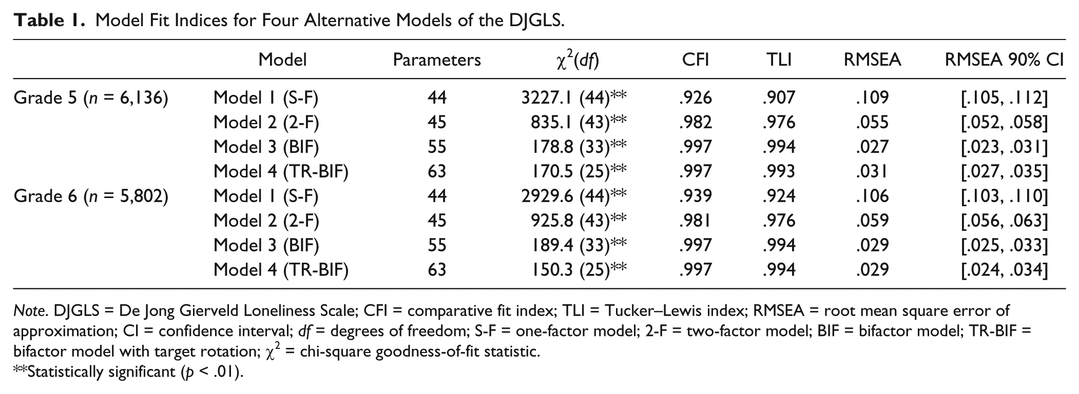
Note. DJGLS = De Jong Gierveld Loneliness Scale; CFI = comparative fit index; TLI = Tucker–Lewis index; RMSEA = root mean square error of approximation; CI = confidence interval; df = degrees of freedom; S-F = one-factor model; 2-F = two-factor model; BIF = bifactor model; TR-BIF = bifactor model with target rotation; χ² = chi-square goodness-of-fit statistic.

Statistically significant (p < .01).

Model 1 (the unidimensional structure) was rejected for both waves of research as a poor approximation of the data. The two-factor model (Model 2) was found to be of better fit than the one-factor model, though improvements were observed across all fit indices for the bifactor solution (Model 3).

Interestingly, within both Grades 5 and 6, the ESEM with TR-BIF (Model 4) does not prove to offer better fit to data than the purely BIF (Model 3). The inclusion of potential cross-loadings did not lead, then, to improved model fit to the data. Taking into account Marsh’s recommendation (Marsh et al., 2014; Marsh, Liem, Martin, Morin, & Nagengast, 2011), these results provide support for the supremacy of a strict BIF, that is, that the structure of the DJGLS is best represented by a single-latent factor, and the presence of two subfactors (without cross-loadings).

Reliability

Both the Alpha coefficient and its equivalent for the latent general factor and subfactors (Omega and OmegaS), indicate that (in both waves) the DJGLS and, independently, both subscales are reliable (Alpha > .70, Omega > .70, and OmegaS > .70). The analysis of OmegaH (the index of essential unidimentionality—in both grades >.70) and OmegaHS (which reflects subscale reliability estimates after controlling for the general factor <.50) suggest that interpretation of the subfactors beyond the general factor is inappropriate as little variance exists beyond the general factor. ECV for both grades also suggest that the general factor of the DJGLS accounts for the majority (almost three quarters) of all common variance and that the DJGLS is essentially a unidimensional scale (for details, see Table 2).

Table 2.

Measures of Reliability and Dimensionality in Grade 5 (n = 6,136) and Grade 6 (n = 5,802) of the DJGLS.

	Grade 5			Grade 6
	GF	NSF	PSF	GF	NSF	PSF
Alpha^a	.86	.81	.80	.87	.82	.81
Omega	.93	—	—	.94	—	—
OmegaS	—	.90	.88	—	.91	.89
OmegaH	.77	—	—	.80	—	—
OmegaHS	—	.41	.06	—	.35	.06
ECV	.73	—	—	.76	—	—

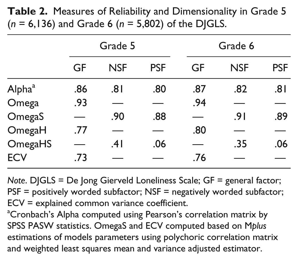
Note. DJGLS = De Jong Gierveld Loneliness Scale; GF = general factor; PSF = positively worded subfactor; NSF = negatively worded subfactor; ECV = explained common variance coefficient.

Cronbach’s Alpha computed using Pearson’s correlation matrix by SPSS PASW statistics. OmegaS and ECV computed based on Mplus estimations of models parameters using polychoric correlation matrix and weighted least squares mean and variance adjusted estimator.

External Validity

Table 3 presents the latent correlations between the general factor of the DJGLS from the strictly BIF (see Model 3 in Table 1) and other variables. As predicted, social self-efficacy, identification with class group, peer acceptance, and parent’s education are negatively related to the loneliness measured by the DJGLS. As expected, positive correlations have been noted between the DJGLS a peer rejection and self-rating loneliness. Higher scores on the DJGLS loneliness scale were obtained by boys than girls, and children from single-parent families, which is also consistent with our hypotheses. Contrary to the expectations, however, there was no statistically significant relationship between the DJGLS and SES of the parent’s (HISEI).

Table 3.

Correlations for General Factor DJGLS Based on a Bifactor Model and External Variables (n = 6,136).

Variable	1	2	3	4	5	6	7	8	9
1. Loneliness (DJGLS)^cl
2. Gender (0 = boys; 1 = girls)^b	−.06**
3. Family structure (0 = two-parent; 1 = one-parent)^b	.09**	−.01
4. Parents social status (HISEI)^cm	−.02	−.02	−.14**
5. Parents education (HEDU)^cm	−.03*	−.03	−.19**	.74**
6. Self-rating Loneliness^o	.84**	.06**	.09**	−.03	−.04*
7. Social self-efficacy (S-SEQ-C)^cl	−.67**	.11**	−.07**	.07**	.10**	−.61**
8. Identification with class group (PSIS)^cl	−.83**	.04*	−.10**	.02	.05**	−.82**	.81**
9. Peer acceptance (PinDC)^cm	−.28**	.02	−.12**	.06**	.07**	−.35**	.29**	.41**
10. Peer rejection (NinDC)^cm	.24**	−.19**	.13**	−.13**	−.14**	.29**	−.25**	−.39**	−.46**

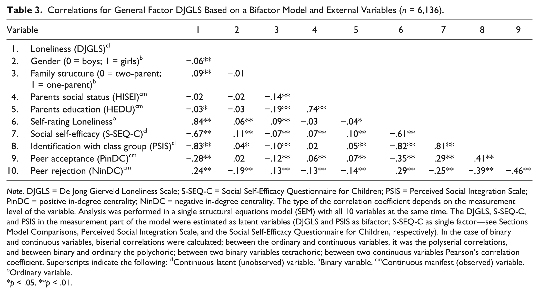
Note. DJGLS = De Jong Gierveld Loneliness Scale; S-SEQ-C = Social Self-Efficacy Questionnaire for Children; PSIS = Perceived Social Integration Scale; PinDC = positive in-degree centrality; NinDC = negative in-degree centrality. The type of the correlation coefficient depends on the measurement level of the variable. Analysis was performed in a single structural equations model (SEM) with all 10 variables at the same time. The DJGLS, S-SEQ-C, and PSIS in the measurement part of the model were estimated as latent variables (DJGLS and PSIS as bifactor; S-SEQ-C as single factor—see Sections Model Comparisons, Perceived Social Integration Scale, and the Social Self-Efficacy Questionnaire for Children, respectively). In the case of binary and continuous variables, biserial correlations were calculated; between the ordinary and continuous variables, it was the polyserial correlations, and between binary and ordinary the polychoric; between two binary variables tetrachoric; between two continuous variables Pearson’s correlation coefficient. Superscripts indicate the following: ^clContinuous latent (unobserved) variable. ^bBinary variable. ^cmContinuous manifest (observed) variable. ^oOrdinary variable.

p < .05. **p < .01.

Longitudinal Invariance

Table 4 shows the fit statistics for the measurement invariance models. The fit indices indicated a good fit to the data (i.e., RMSEA ≤ .06 and TLI/CFI ≥ .95). If the RMSEA and CFI values do not deteriorate in the more constrained models (i.e., the loading and loadings/threshold invariance models), this is indicative of measurement invariance. As can be seen, there was no decrease in fit for the more restricted models’ comparisons. The differences are well below the suggested cutoff points for establishing measurement invariance (a decrease in CFI of ≥ .002 and an increase in RMSEA of ≥ .007).

Table 4.

Model Fit Indices for the Longitudinal Measurement Invariance Models of the DJGLS (n = 6,292).

Model	Parameters	χ²(df)	TLI	CFI	ΔCFI	RMSEA	RMSEA 90% CI	ΔRMSEA
Configural^a	124	459.3 (173)**	.995	.997	—	.016	[.014, .018]	—
Metric^b	106	477.0 (191)**	.996	.997	.000	.015	[.014, .017]	−.001
Scalar^c	90	503.0 (207)**	.996	.997	.000	.015	[.013, .017]	−.000

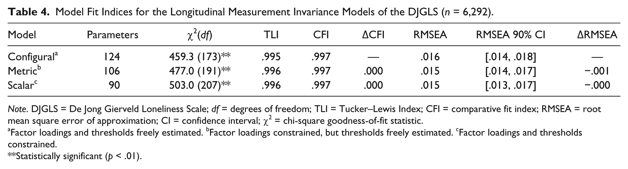
Note. DJGLS = De Jong Gierveld Loneliness Scale; df = degrees of freedom; TLI = Tucker–Lewis Index; CFI = comparative fit index; RMSEA = root mean square error of approximation; CI = confidence interval; χ² = chi-square goodness-of-fit statistic.

Factor loadings and thresholds freely estimated. ^bFactor loadings constrained, but thresholds freely estimated. ^cFactor loadings and thresholds constrained.

Statistically significant (p < .01).

Table 5 shows the factor loadings from the model of scalar invariance of the DJGLS. Almost all loadings for standardized GF are above .50 (with the exception of Item 9) and the mean value of the loadings is .65 in Grade 5 and .67 in Grade 6. At the same time, most of the loadings on subfactors do not exceed .50 (the mean for negatively worded subfactor is .46 in Grade 5 and .45 in Grade 6 and for positively worded subfactor, .29 in Grade 5 and .26 Grade 6). Only in the case of Item 9, the value of loading on the subfactor was higher than on the GF (in both waves). The arrangement of obtained loadings confirms that the DJGLS measures the intensity of a global feeling of loneliness rather than two of its dimensions.

Table 5.

Factor Loadings (Unstandardized and Standardized) From Scalar Model for Grades 5 and 6 (n = 6,292).

	GF	NSF	PSF
Lone1	0.53 (.56/.59)		0.65 (.36/.32)
Lone2	0.89 (.75/.78)	1.00 (.31/.31)
Lone3	0.78 (.64/.66)	1.63 (.50/.49)
Lone4	1.00 (.75/.78)		1.00 (.39/.35)
Lone5	1.03 (.72/.74)	1.86 (.49/.46)
Lone6	0.54 (.54/.56)	1.23 (.46/.44)
Lone7	0.83 (.74/.76)		0.60 (.28/.25)
Lone8	0.59 (.62/.65)		0.53 (.29/.26)
Lone9	0.25 (.29/.32)	1.22 (.52/.53)
Lone10	0.95 (.71/.73)	1.74 (.48/.46)
Lone11	0.89 (.78/.82)		0.25 (.11/.10)

Note. GF = general factor; PSF = positively worded subfactor; NSF = negatively worded subfactor; before parentheses unstandardized factor loadings, in parentheses standardized loadings, first for Grade 5, and second for Grade 6.

Longitudinal Stability and Change

The correlation coefficient between the general factor of the DJGLS in Grade 5 and Grade 6 was .65 (SE = .01, p < .001) which, accepting Cohen’s (1988) recommendation, indicates a high measurement stability year on year. Additionally, the latent means of the general factor of the DJGLS in Time 2 (Grade 6) were compared with the mean of Time1 (Grade 5) fixed to zero. Compared with Grade 5, loneliness in Grade 6 had a higher mean (M = .18, SE = .05, p < .01), pointing to an increase in loneliness over time.

Discussion

The present investigation is the first study designed to examine the factor structures, reliability, external validity, longitudinal invariance, and stability of the DJGLS among school age children.

Consistent with the initial prediction, the results of the current study suggest that the structure of loneliness among school children, as measured by the DJGLS, is best conceptualized as a BIF with orthogonal general and two specific factors. Moreover, results indicate that approximately 75% of the common variance can be explained by the general factor, suggesting that there is very little reliable variance beyond that due to the general latent trait. This result, combined with high values of Omega and OmegaH coefficients for the general factor and low values of OmegaHS for subfactors, indicates that the DJGLS is essentially unidimensional. This, in turn, leads to the conclusion that subfactors do not yield enough precise measures of unique aspects of loneliness to be useful in practical applications. Researchers using the DJGLS to measure the two types of loneliness (social and emotional) must keep in mind that most of the true score variance in these two subscales is accounted for by the general loneliness factor.

Statistically, significant positive correlations with peer rejection and self-ratings of loneliness, negative correlations with parent’s education, social self-efficacy, identification with class group, and peer acceptance, and higher loneliness within boys, and children from single parent families provide support for the validity of the DJGLS. At the same time, correlations between loneliness and gender, and whether a child is brought up in a one- or two-parent family, and parent’s education although statistically significant, are very weak and might be considered as trivial effects (Cohen, 1988).

Gender or number of parents cannot, therefore, be considered as variables which substantially differentiate loneliness levels in early adolescence, whereas when it comes to gender the result can be considered consistent with other research (see, e.g., Maes et al., 2017); in the case of the second variable, we could expect a stronger relationship, taking into account that children brought up in single-parent families usually have a lower level of social competences (Guidubaldi & Perry, 1984) and less extensive social networks at their disposal (Samuelsson, 1995, 1997).

A rather minor relevance of factors related to the “structural” aspects of the family is additionally confirmed by the fact that contrary to expectations, the intensity of loneliness was unrelated to socioeconomic position of the parent’s. Additionally, HISEI does not correlate with a sense of connection with class peers and parents’ education is only marginally related to it. The weak link between SES and various measures of assessing the quality of peer relations appears to be more systematic than random.

It is interesting to the extent that our analysis suggests, as do the results of previous studies, that higher levels of SES promotes better self-assessment of social competence (Guidubaldi & Perry, 1984), greater peer acceptance and a lower level of peer rejection (Asher & Wheeler, 1985), which is in turn directly related to the feeling of loneliness. So, we can hypothesize that the SES of a pupil’s family translates into a level of loneliness not so much directly as indirectly, through social competence, acceptance, and rejection by peers. Testing this hypothesis was, however, beyond the scope of the present study. Generally speaking, based on our study, we cannot answer the question as to why, contrary to our expectations, higher SES is not associated with lower levels of loneliness.

The longitudinal confirmatory factor analysis indicated that the structure of the DJGLS is stable over time, that is, the scale is invariant in the sense that factor loadings and item thresholds are the same through both times. Our longitudinal study also revealed that the relative order of individuals in loneliness scores was also rather stable, that is, the correlations between general factor in Grades 5 and 6 was high (r = .69), which was contrary to expectations (see, the Longitudinal Stability and Change section). This may be due to the use of latent variables in the discussed analysis, and not, as in previous studies, observable variables. Correlations between the latter, in addition to information on the trait of interest, also included the component to the measurement error (Gallini, 1983), which reduces the size of the estimated correlations (Milanzi, Molenberghs, Alonso, Verbeke, & De Boeck, 2015).

According to the results of previous studies indicating a deterioration in the perception of the quality of peer relationships during elementary school (see the Longitudinal Stability and Change section), this analysis also shows an increase in the level of loneliness between Grades 5 and 6, which confirms the suitability of the DJGLS to the measurement of the sense of social isolation among children.

There were several limitations to this study. The research project from which the data discussed here originates used DJGLS only in two waves of research, separated by a period of 1 year. In order to capture the “resistance” of the scale to short-term fluctuations (its measurement stability), which are not due to changes in the phenomenon under analysis, tests at shorter intervals, for example, after 2 weeks, 1 month, and 3 months should be carried out.

This research was conducted among pupils of Grades 5 and 6, which in the Polish education system are the final years of elementary school. It would certainly be worth replicating the results, beginning with longitudinal studies among pupils at the earlier developmental stages (e.g., among 9–year-olds) and continue the research with every subsequent year of study. This would allow us to see whether reliable results can be obtained with the DJGLS used among children at earlier stages of development, that is, finding out whether it is not too difficult.

Including pupils at an earlier stage of learning in research, while also increasing the number of research points, would provide an opportunity for checking the ways in which a sense of social isolation changes with an increase of pupils’ cognitive capabilities and improvement in their social skills.

Unfortunately, the study’s external validity may be limited. Apart from direct questioning, the validation process did not include any other questionnaires designed to study loneliness. Therefore, in order to consolidate the thesis about the external validity of the DJGLS, any subsequent analyses should investigate the relationships occurring between the results reached with the DJGLS and other results obtained with the use of different tools used to measure loneliness, mostly those that have been created for the purposes of research in the school environment, for example, the LSDS (Asher & Wheeler, 1985) or the Loneliness in Context Questionnaire for Children (Weeks & Asher, 2012).

Overall, our findings, based on a large, representative sample of Polish children, demonstrate that the DJGLS is a measure of loneliness, which is brief, essentially unidimensional, reliable, valid, and stable over time. This implies that the DJGLS could be used as the measure of loneliness in children which does not include references to school context, enabling research that goes beyond the school period as well as the comparison of the intensity of loneliness in this group with different age groups.

Footnotes

Declaration of Conflicting Interests

The author(s) declared no potential conflicts of interest with respect to the research, authorship, and/or publication of this article.

Funding

The author(s) received no financial support for the research, authorship, and/or publication of this article.

Supplemental Material

Supplemental material for this article is available online.

Notes

References

Anderson

T. W.

(1957). Maximum likelihood estimates for a multivariate normal distribution when some observations are missing. Journal of the American Statistical Association, 52, 200-203. doi:10.1080/01621459.1957.10501379

Asher

S. R.

Hymel

Renshaw

P. D.

(1984). Loneliness in children. Child Development, 55, 1456-1464. doi:10.2307/1130015

Asher

S. R.

Weeks

M. S.

(2013). Loneliness and belongingness in the college years. In Coplan

R. J.

Bowker

J. C.

(Eds.), The handbook of solitude (pp. 283-301). Hoboken, NJ: John Wiley.

Asher

S. R.

Wheeler

V. A.

(1985). Children’s loneliness: A comparison of rejected and neglected peer status. Journal of Consulting and Clinical Psychology, 53, 500-505. doi:10.1037/0022-006X.53.4.500

Asparouhov

Muthén

B. O.

(2009). Exploratory structural equation modeling. Structural Equation Modeling: A Multidisciplinary Journal, 16, 397-438. doi:10.1080/10705510903008204

Beauducel

Herzberg

P. Y.

(2006). On the performance of maximum likelihood versus means and variance adjusted weighted least squares estimation in CFA. Structural Equation Modeling: A Multidisciplinary Journal, 13, 186-203. doi:10.1207/s15328007sem1302_2

Bentler

P. M.

(1990). Comparative fit indexes in structural models. Psychological Bulletin, 107, 238-246. doi:10.1037/0033-2909.107.2.238

Brown

T. A.

(2006). Confirmatory factor analysis for applied research. New York, NY: Guilford Press.

Browne

M. W.

(1972a). Oblique rotation to a partially specified target. British Journal of Mathematical and Statistical Psychology, 25, 207-212. doi:10.1111/j.2044-8317.1972.tb00492.x

10.

Browne

M. W.

(1972b). Orthogonal rotation to a partially specified target. British Journal of Mathematical and Statistical Psychology, 25, 115-120. doi:10.1111/j.2044-8317.1972.tb00482.x

11.

Browne

M. W.

(2001). An overview of analytic rotation in exploratory factor analysis. Multivariate Behavioral Research, 36, 111-150. doi:10.1207/S15327906MBR3601_05

12.

Bukowski

W. M.

Brendgen

Vitaro

(2007). Peer and socialization: Effects on externalizing and internalizing problems. In Grusec

J. E.

Hastings

P. D.

(Eds.), Handbook of socialization: Theory and research (pp. 355-381). New York, NY: Guilford Press.

13.

Buz

Urchaga

Polo

M. E.

(2014). Análisis factorial confirmatorio de la escala de soledad de De Jong Gierveld en personas mayores españolas [Factor structure of the De Jong Gierveld loneliness scale in Spanish elderly adults]. Anales de Psicología, 30, 588-596. doi:10.6018/analesps.30.2.148371

14.

Byrne

B. M.

(2011). Structural equation modeling with Mplus: Basic concepts, applications, and programming. New York, NY: Routledge.

15.

Cacioppo

J. T.

Cacioppo

Boomsma

D. I.

(2014). Evolutionary mechanisms for loneliness. Cognition and Emotion, 28, 3-21. doi:10.1080/02699931.2013.837379

16.

Cassidy

Asher

S. R.

(1992). Loneliness and peer relations in young children. Child Development, 63, 350-365. doi:10.1111/j.1467-8624.1992.tb01632.x

17.

Cattan

White

Bond

Learmouth

(2005). Preventing social isolation and loneliness among older people: A systematic review of health promotion interventions. Ageing & Society, 25, 41-67. doi:10.1017/S0144686X04002594

18.

Çivitci

Fiyakali

N. C.

(2009). Loneliness and life satisfaction in adolescents with divorced and non-divorced parents. Educational Sciences: Theory & Practice, 9, 513-525.

19.

Cohen

(1988). Statistical power analysis for the behavioral sciences (2nd ed.). Hillsdale, NJ: Lawrence Erlbaum.

20.

Coie

J. D.

Dodge

K. A.

Coppotelli

(1982). Dimensions and types of social status: A cross-age perspective. Developmental Psychology, 18, 557-570.

21.

Cronbach

L. J.

(1951). Coefficient alpha and the internal structure of tests. Psychometrika, 16, 297-334. doi:10.1007/BF02310555

22.

de Jong Gierveld

. (1987). Developing and testing a model of loneliness. Journal of Personality and Social Psychology, 53, 119-128. doi:10.1037//0022-3514.53.1.119

23.

de Jong Gierveld

Kamphuls

. (1985). The development of a Rasch-type loneliness scale. Applied Psychological Measurement, 9, 289-299. doi:10.1177/014662168500900307

24.

de Jong Gierveld

van Tilburg

. (1999). Living arrangements of older adults in the Netherlands and Italy: Coresidence values and behaviour and their consequences for loneliness. Journal of Cross-Cultural Gerontology, 14, 1-24.

25.

de Jong Gierveld

van Tilburg

. (2010). The De Jong Gierveld short scales for emotional and social loneliness: Tested on data from 7 countries in the UN generations and gender surveys. European Journal of Ageing, 7, 121-130. doi:10.1007/s10433-010-0144-6

26.

de Jong Gierveld

van Tilburg

Dykstra

P. A

. (2006). Loneliness and social isolation. In Perlman

Vangelisti

(Eds.), Cambridge handbook of personal relationships (pp. 485-500). Cambridge, England: Cambridge University Press.

27.

Dimitrov

D. M.

(2010). Testing for factorial invariance in the context of construct validation. Measurement and Evaluation in Counseling and Development, 43, 121-149. doi:10.1177/0748175610373459

28.

Dodeen

(2014). The effects of positively and negatively worded items on the factor structure of the UCLA Loneliness Scale. Journal of Psychoeducational Assessment, 33, 259-267. doi:10.1177/0734282914548325

29.

Dolata

Hawrot

Humenny

Jasińska-Maciążek

Koniewski

Majkut

(2014). Kontekstowy model efektywności nauczania po pierwszym etapie edukacyjnym. Edukacyjna Wartość Dodana [The contextual model of teaching efficiency after the first educational stage. Educational Value Added]. Warsaw, Poland: Instytut Badań Edukacyjnych.

30.

Dolata

Hawrot

Humenny

Jasińska-Maciążek

Koniewski

Majkut

. . . Otręba-Szklarczyk

(2015). (Ko)warianty efektywności nauczania: wyniki badania w klasach IV-VI [(Co-)Variants of teaching efficiency: Results of research within the 4th-6th Grades]. Warsaw, Poland: Instytut Badań Edukacyjnych.

31.

Dweck

C. S.

(2002). The development of ability conceptions. In Wigfield

Eccles

J. S.

(Eds.), Development of achievement motivation (pp. 57-88). San Diego, CA: Academic Press.

32.

Dykstra

P. A.

de Jong Gierveld

(2004). Gender and marital-history differences in emotional and social loneliness among Dutch older adults. Canadian Journal on Aging/La Revue Canadienne du Vieillissement, 23, 141-155. doi:10.1353/cja.2004.0018

33.

Dykstra

P. A.

Fokkema

(2007). Social and emotional loneliness among divorced and married men and women: Comparing the deficit and cognitive perspectives. Basic and Applied Social Psychology, 29, 1-12. doi:10.1080/01973530701330843

34.

Ebesutani

Drescher

C. F.

Reise

S. P.

Heiden

Hight

T. L.

Damon

J. D.

Young

(2012). The importance of modeling method effects: Resolving the (uni)dimensionality of the loneliness questionnaire. Journal of Personality Assessment, 94, 186-195. doi:10.1080/00223891.2011.627967

35.

Enders

C. K.

Bandalos

D. L.

(2001). The relative performance of full information maximum likelihood estimation for missing data in structural equation models. Structural Equation Modeling: A Multidisciplinary Journal, 8, 430-457. doi:10.1207/S15328007SEM0803_5

36.

Flora

D. B.

Curran

P. J.

(2004). An empirical evaluation of alternative methods of estimation for confirmatory factor analysis with ordinal data. Psychological Methods, 9, 466-491. doi:10.1037/1082-989X.9.4.466

37.

Freeman

L. C.

(1978). Centrality in social networks conceptual clarification. Social Networks, 1, 215-239. doi:10.1016/0378-8733(78)90021-7

38.

Furman

Buhrmester

(1992). Age and sex differences in perceptions of networks of personal relationships. Child Development, 63, 103-115. doi:10.1111/j.1467-8624.1992.tb03599.x

39.

Galanaki

E. P.

Kalantzi-Azizi

(1999). Loneliness and social dissatisfaction: Its relation with children’s self-efficacy for peer interaction. Child Study Journal, 29, 1-22.

40.

Gallini

(1983). Misspecifications that can result in path analysis structures. Applied Psychological Measurement, 7, 125-137.

41.

Graham

J. W.

(2009). Missing data analysis: Making it work in the real world. Annual Review of Psychology, 60, 549-576. doi:10.1146/annurev.psych.58.110405.085530

42.

Grygiel

(2015). Test ukrytej struktury kwestionariusza “Poczucie Integracji Rówieśniczej.” Częściowo konfirmacyjny model podwójnego czynnika z ładunkami krzyżowymi [The test of latent structure of the Perceived Peer Integration Questionnaire. Partially confirmatory bifactor model with cross-loadings]. In Niemierko

Szmigel

M. K.

(Eds.), Zastosowania diagnozy edukacyjnej [Applications of educational diagnosis] (pp. 438-458). Krakow: Poland: Polskie Towarzystwo Diagnostyki Edukacyjnej.

43.

Grygiel

Humenny

Rębisz

Bajcar

Świtaj

(2018). Peer rejection and perceived quality of relations with schoolmates among children with ADHD. Journal of Attention Disorders, 22, 738-751.

44.

Grygiel

Humenny

Rębisz

Świtaj

Sikorska

(2013). Validating the Polish adaptation of the 11-item De Jong Gierveld Loneliness Scale. European Journal of Psychological Assessment, 29, 129-139. doi:10.1027/1015-5759/a000130

45.

Guidubaldi

Perry

J. D.

(1984). Divorce, socioeconomic status, and children’s cognitive-social competence at school entry. American Journal of Orthopsychiatry, 54, 459-468. doi:10.1111/j.1939-0025.1984.tb01511.x

46.

Haeberlin

Moser

Bless

Klaghofer

(1989). Integration in die Schulklasse: Fragebogen zur Erfassung von Dimensionen der Integration von Schülern: FDI 4-6 [Integration in the classroom: Questionnaire for the assessment of pupil’s dimensions of integration: QDI 4-6]. Bern, Switzerland: Haupt.

47.

Hartup

W. W.

Stevens

(1997). Friendships and adaptation in the life course. Psychological Bulletin, 121, 355-370. doi:10.1037/0033-2909.121.3.355

48.

Heinrich

L. A.

Gullone

(2006). The clinical significance of loneliness: A literature review. Clinical Psychology Review, 26, 695-718. doi:10.1016/j.cpr.2006.04.002

49.

Higbee

K. R.

Roberts

R. E.

(1994). Reliability and validity of a brief measure of loneliness with Anglo-American and Mexican American adolescents. Hispanic Journal of Behavioral Sciences, 16, 459-474. doi:10.1177/07399863940164005

50.

Holgado–Tello

F. P.

Chacón–Moscoso

Barbero–García

Vila–Abad

(2010). Polychoric versus Pearson correlations in exploratory and confirmatory factor analysis of ordinal variables. Quality & Quantity, 44, 153-166. doi:10.1007/s11135-008-9190-y

51.

Horn

J. L.

Mcardle

J. J.

(1992). A practical and theoretical guide to measurement invariance in aging research. Experimental Aging Research, 18, 117-144. doi:10.1080/03610739208253916

52.

Howard

J. L.

Gagne

Morin

A. J. S.

Forest

(2018). Using bifactor exploratory structural equation modeling to test for a continuum structure of motivation. Journal of Management, 44, 2638-2664.

53.

Howe

T. R.

Parke

R. D.

(2001). Friendship quality and sociometric status: Between-group differences and links to loneliness in severely abused and nonabused children. Child Abuse & Neglect, 25, 585-606. doi:10.1016/S0145-2134(01)00230-7

54.

Humenny

Grygiel

(2015). Poza ścisłą jedno- i wielowymiarowość. Struktura czynnikowa skali samotności de Jong Gierveld wśród dzieci [Beyond strict uni - and multidimensionality. The factorial structure of the De Jong Gierveld Loneliness Scale among children]. In Pokropek

(Ed.), Modele cech ukrytych w badaniach edukacyjnych, psychologii i socjologii. Teoria i zastosowania [Models of latent traits in educational, psychological and sociological research. Theory and praxis] (pp. 400-424). Warsaw, Poland: Instytut Badań Edukacyjnych.

55.

Jobe-Shields

Cohen

Parra

G. R.

(2011). Patterns of change in children’s loneliness: Trajectories from third through fifth grades. Merrill-Palmer Quarterly, 57, 25-47.

56.

Jose

P. E.

Lim

B. T. L.

(2014). Social connectedness predicts lower loneliness and depressive symptoms over time in adolescents. Open Journal of Depression, 3, 154-163. doi:10.4236/ojd.2014.34019

57.

Ladd

G. W.

Burgess

K. B.

(1999). Charting the relationship trajectories of aggressive, withdrawn, and aggressive/withdrawn children during early grade school. Child Development, 70, 910-929. doi:10.1111/1467-8624.00066

58.

Ladd

G. W.

Ettekal

(2013). Peer-related loneliness across early to late adolescence: Normative trends, intra-individual trajectories, and links with depressive symptoms. Journal of Adolescence, 36, 1269-1282. doi:10.1016/j.adolescence.2013.05.004

59.

Larson

R. W.

(1999). The uses of loneliness in adolescence. In Rotenberg

K. J.

Hymel

(Eds.), Loneliness in childhood and adolescence (pp. 244-262). Cambridge, England: Cambridge University Press.

60.

Larson

R. W.

Richards

M. H.

Moneta

Holmbeck

Duckett

(1996). Changes in adolescents’ daily interactions with their families from ages 10 to 18: Disengagement and transformation. Developmental Psychology, 32, 744-754. doi:10.1037/0012-1649.32.4.744

61.

Laursen

Hartl

A. C.

(2013). Understanding loneliness during adolescence: Developmental changes that increase the risk of perceived social isolation. Journal of Adolescence, 36, 1261-1268. doi:10.1016/j.adolescence.2013.06.003

62.

Levitt

M. J.

Guacci-Franco

Levitt

J. L.

(1993). Convoys of social support in childhood and early adolescence: Structure and function. Developmental Psychology, 29, 811-818. doi:10.1037/0012-1649.29.5.811

63.

C.-H.

(2016). Confirmatory factor analysis with ordinal data: Comparing robust maximum likelihood and diagonally weighted least squares. Behavior Research Methods, 48, 936-949. doi:10.3758/s13428-015-0619-7

64.

Little

R. J. A.

(1988). A Test of Missing Completely at Random for Multivariate Data with Missing Values. Journal of the American Statistical Association, 83, 1198–1202. doi: 10.1080/01621459.1988.10478722

65.

Little

T. D.

(2013). Longitudinal structural equation modeling. New York, NY: Guilford Press.

66.

Maes

Klimstra

Van den Noortgate

Goossens

(2015). Factor structure and measurement invariance of a multidimensional loneliness scale: Comparisons across gender and age. Journal of Child and Family Studies, 24, 1829-1837. doi:10.1007/s10826-014-9986-4

67.

Maes

Van den Noortgate

Vanhalst

Beyers

Goossens

(2017). The Children’s Loneliness Scale: Factor structure and construct validity in Belgian children. Assessment, 24, 244-251.

68.

Mahon

N. E.

Yarcheski

T. J.

Cannella

B. L.

Hanks

M. M.

(2006). A meta-analytic study of predictors for loneliness during adolescence. Nursing Research, 55, 308-315.

69.

Marcoen

Goossens

Caes

(1987). Loneliness in pre-through late adolescence: Exploring the contributions of a multidimensional approach. Journal of Youth and Adolescence, 16, 561-577. doi:10.1007/bf02138821

70.

Marsh

H. W.

Hau

K.-T.

Grayson

(2005). Goodness of fit evaluation in structural equation modeling. In Maydeu-Olivares

McArdle

J. J.

McDonald

R. P.

(Eds.), Contemporary psychometrics: A festschrift for Roderick P. McDonald (pp. 275-340). Mahwah, NJ: Lawrence Erlbaum.

71.

Marsh

H. W.

Liem

G. A. D.

Martin

A. J.

Morin

A. J. S.

Nagengast

(2011). Methodological measurement fruitfulness of exploratory structural equation modeling (ESEM): New approaches to key substantive issues in motivation and engagement. Journal of Psychoeducational Assessment, 29, 322-346. doi:10.1177/0734282911406657

72.

Marsh

H. W.

Morin

A. J. S.

Parker

P. D.

Kaur

(2014). Exploratory structural equation modeling: An integration of the best features of exploratory and confirmatory factor analysis. Annual Review of Clinical Psychology, 10, 85-110. doi:10.1146/annurev-clinpsy-032813-153700

73.

Marsh

H. W.

Shavelson

(1985). Self-concept: Its multifaceted, hierarchical structure. Educational Psychologist, 20, 107-123. doi:10.1207/s15326985ep2003_1

74.

McDonald

R. P.

(1999). Test theory: A unified treatment. Mahwah, NJ: Lawrence Erlbaum.

75.

Meade

A. W.

Johnson

E. C.

Braddy

P. W.

(2008). Power and sensitivity of alternative fit indices in tests of measurement invariance. Journal of Applied Psychology, 93, 568-592. doi:10.1037/0021-9010.93.3.568

76.

Milanzi

Molenberghs

Alonso

Verbeke

De Boeck

(2015). Reliability measures in item response theory: Manifest versus latent correlation functions. British Journal of Mathematical and Statistical Psychology, 68, 43-64. doi:10.1111/bmsp.12033

77.

Millsap

R. E.

(2011). Statistical approaches to measurement invariance. New York, NY: Psychology Press.

78.

Morin

A. J. S.

Arens

A. K.

Marsh

H. W.

(2015). A bifactor exploratory structural equation modeling framework for the identification of distinct sources of construct-relevant psychometric multidimensionality. Structural Equation Modeling: A Multidisciplinary Journal, 23, 116-139. doi:10.1080/10705511.2014.961800

79.

Morin

A. J. S.

Marsh

H. W.

Nagengast

(2013). Exploratory structural equation modeling. In Hancock

G. R.

Mueller

R. O.

(Eds.), Structural equation modeling: A second course (2nd ed., pp. 395-436). Charlotte, NC: Information Age.

80.

Mouratidis

A. A.

Sideridis

G. D.

(2009). On social achievement goals: Their relations with peer acceptance, classroom belongingness, and perceptions of loneliness. Journal of Experimental Education, 77, 285-308. doi:10.3200/JEXE.77.3.285-308

81.

Muris

(2001). A brief questionnaire for measuring self-efficacy in youths. Journal of Psychopathology and Behavioral Assessment, 23, 145-149. doi:10.1023/A:1010961119608

82.

Muris

(2002). Relationships between self-efficacy and symptoms of anxiety disorders and depression in a normal adolescent sample. Personality and Individual Differences, 32, 337-348. doi:10.1016/S0191-8869(01)00027-7

83.

Muthén

B. O.

Muthén

L. K.

(1998-2015). Mplus user’s guide (7th ed.). Los Angeles, CA: Author.

84.

Nunnally

J. C.

(1978). Psychometric theory (2d ed.). New York, NY: McGraw-Hill.

85.

Olatunji

B. O.

Ebesutani

Reise

S. P.

(2015). A bifactor model of disgust proneness: Examination of the Disgust Emotion Scale. Assessment, 22, 248-262. doi:10.1177/1073191114541673

86.

Olsson

(1979). Maximum likelihood estimation of the polychoric correlation coefficient. Psychometrika, 44, 443–460. doi: 10.1007/BF02296207

87.

Parker

J. G.

Asher

S. R.

(1993). Friendship and friendship quality in middle childhood: Links with peer group acceptance and feelings of loneliness and social dissatisfaction. Developmental Psychology, 29, 611-621. doi:10.1037/0012-1649.29.4.611

88.

Parkhurst

J. T.

Hopmeyer-Gorman

(1999). Developmental change in the sources of loneliness in childhood and adolescence: Constructing a theoretical model. In Rotenberg

Hymel

(Eds.), Loneliness in childhood and adolescence (pp. 56-80). Cambridge, England: Cambridge University Press.

89.

Penning

M. J.

Liu

Chou

P. H. B.

(2014). Measuring loneliness among middle-aged and older adults: The UCLA and de Jong Gierveld loneliness scales. Social Indicators Research, 118, 1147-1166. doi:10.1007/s11205-013-0461-1

90.

Peplau

L. A.

(1982). Perspectives on loneliness. In Peplau

L. A.

Perlman

(Eds.), Loneliness: A sourcebook of current theory, research, and therapy (pp. 135-151). New York, NY: Wiley Interscience.

91.

Perlman

, (1990, 10-14 August). Age differences in loneliness: A meta-analysis. Paper presented at the 98th Annual Convention of the American Psychological Association, Boston, MA.

92.

Perlman

Landolt

M. A.

(1999). Examination of loneliness in children–adolescents and in adults: two solitudes or unified enterprise? In Rotenberg

K. J.

Hymel

(Eds.), Loneliness in childhood and adolescence (pp. 325–347). Cambridge, England: Cambridge University Press.

93.

Pfeifer

J. H.

Peake

S. J.

(2012). Self-development: Integrating cognitive, socioemotional, and neuroimaging perspectives. Developmental Cognitive Neuroscience, 2, 55-69. doi:10.1016/j.dcn.2011.07.012

94.

Post

W. J.

van Duijn

M. A. J.

van Baarsen

(2001). Single-peaked or monotone tracelines? On the choice of an IRT model for scaling data. In Boomsma

van Duijn

M. A. J.

Snijders

T. A. B.

(Eds.), Essays on item response theory (Vol. 157, pp. 391-414). New York, NY: Springer.

95.

Qualter

(2003). Loneliness in children and adolescents: What do schools and teachers need to know and how can they help? Pastoral Care in Education, 21(2), 10-18. doi:10.1111/1468-0122.00257

96.

Quay

L. C.

(1992). Personal and family effects on loneliness. Journal of Applied Developmental Psychology, 13, 97-110. doi:10.1016/0193-3973(92)90008-6

97.

Quinn

H. O.

(2014). Bifactor models, explained common variance (ECV), and the usefulness of scores from unidimensional item response theory analyses (Master’s thesis). Retrieved from https://cdr.lib.unc.edu/indexablecontent/uuid:efa83eb6-add5-4d21-a252-823ca4a043f3

98.

Reise

S. P.

Bonifay

W. E.

Haviland

M. G.

(2013). Scoring and modeling psychological measures in the presence of multidimensionality. Journal of Personality Assessment, 95, 129-140. doi:10.1080/00223891.2012.725437

99.

Reise

S. P.

Moore

Maydeu-Olivares

(2011). Target rotations and assessing the impact of model violations on the parameters of unidimensional item response theory models. Educational and Psychological Measurement, 71, 684-711. doi:10.1177/0013164410378690

100.

Reise

S. P.

Scheines

Widaman

K. F.

Haviland

M. G.

(2013). Multidimensionality and structural coefficient bias in structural equation modeling: A bifactor perspective. Educational and Psychological Measurement, 73, 5-26. doi:10.1177/0013164412449831

101.

Revelle

Zinbarg

R. E.

(2009). Coefficients alpha, beta, omega, and the glb: Comments on Sijtsma. Psychometrika, 74, 145-154. doi:10.1007/s11336-008-9102-z

102.

Revenson

T. A.

(1986). Debunking the myth of loneliness in late life. In Seidman

Rappaport

(Eds.), Redefining social problems (pp. 115-135). New York, NY: Springer.

103.

Rodriguez

Reise

S. P.

Haviland

M. G.

(2015). Applying bifactor statistical indices in the evaluation of psychological measures. Journal of Personality Assessment, 98, 1-15. doi:10.1080/00223891.2015.1089249

104.

Russell

D. W.

(1996). UCLA Loneliness Scale (Version 3): Reliability, validity, and factor structure. Journal of Personality Assessment, 66, 20-40. doi:10.1207/s15327752jpa6601_2

105.

Samuelsson

(1995). Children’s social networks and their association with behavioural disturbances in single-parent families: A comparison between a clinical group and a control group. Nordic Journal of Psychiatry, 49, 275-284. doi:10.3109/08039489509011917

106.

Samuelsson

(1997). Social networks of children in single-parent families: Differences according to sex, age, socioeconomic status and housing-type and their associations with behavioural disturbances. Social Networks, 19, 113-127. doi:10.1016/S0378-8733(95)00284-7

107.

Steiger

J. H.

(1990). Structural model evaluation and modification: An interval estimation approach. Multivariate Behavioral Research, 25, 173-180. doi:10.1207/s15327906mbr2502_4

108.

Stephan

Fäth

Lamm

(1988). Loneliness as related to various personality and environmental measures: Research with the German adaptation of the UCLA Loneliness Scale. Social Behavior and Personality, 16, 169-174. doi:10.2224/sbp.1988.16.2.169

109.

Stout

W. F.

(1987). A nonparametric approach for assessing latent trait unidimensionality. Psychometrika, 52, 589-617. doi:10.1007/BF02294821

110.

Stout

W. F.

(1990). A new item response theory modeling approach with applications to unidimensionality assessment and ability estimation. Psychometrika, 55, 293-325. doi:10.1007/BF02295289

111.

Szumski

Karwowski

(2015). Emotional and social integration and the big-fish-little-pond effect among students with and without disabilities. Learning and Individual Differences, 43, 63-74. doi:10.1016/j.lindif.2015.08.037

112.

Ten Berge

J. M. F.

Sočan

. (2004). The greatest lower bound to the reliability of a test and the hypothesis of unidimensionality. Psychometrika, 69, 613-625. doi:10.1007/BF02289858

113.

Thomaes

Reijntjes

Orobio

Castro

Bushman

B. J.

Poorthuis

Telch

M. J.

(2010). I like me if you like me: On the interpersonal modulation and regulation of preadolescents’ state self-esteem. Child Development, 81, 811-825. doi:10.1111/j.1467-8624.2010.01435.x

114.

Trinke

S. J.

Bartholomew

(1997). Hierarchies of attachment relationships in young adulthood. Journal of Social and Personal Relationships, 14, 603-625. doi:10.1177/0265407597145002

115.

Tucker

L. R.

Lewis

(1973). A reliability coefficient for maximum likelihood factor analysis. Psychometrika, 38, 1-10. doi:10.1007/BF02291170

116.

Uruk

A. C.

Demir

(2003). The role of peers and families in predicting the loneliness level of adolescents. Journal of Psychology, 137, 179-193. doi:10.1080/00223980309600607

117.

van Baarsen

Smit

J. H.

Snijders

T. A.

Knipscheer

K. P

. (1999). Do personal conditions and circumstances surrounding partner loss explain loneliness in newly bereaved older adults? Ageing & Society, 19, 441-469.

118.

van Tilburg

de Leeuw

. (1991). Stability of scale quality under various data collection procedures: A mode comparison on the “de Jong-Gierveld Loneliness Scale.” International Journal of Public Opinion Research, 3, 69-85. doi:10.1093/ijpor/3.1.69

119.

van Tilburg

Havens

de Jong Gierveld

. (2004). Loneliness among older adults in the Netherlands, Italy, and Canada: A multifaceted comparison. Canadian Journal on Aging/La Revue Canadienne du Vieillissement, 23, 169-180.

120.

Vandenberg

R. J.

Lance

C. E.

(2000). A review and synthesis of the measurement invariance literature: Suggestions, practices, and recommendations for organizational research. Organizational Research Methods, 3, 4-70. doi:10.1177/109442810031002

121.

Verhaeghen

Salthouse

T. A.

(1997). Meta-analyses of age-cognition relations in adulthood: Estimates of linear and nonlinear age effects and structural models. Psychological Bulletin, 122, 231-249. doi:10.1037//0033-2909.122.3.231

122.

Victor

Scambler

Bond

Bowling

(2000). Being alone in later life: Loneliness, social isolation and living alone. Reviews in Clinical Gerontology, 10, 407-417. doi:10.1017/S0959259800104101

123.

Wasserman

Faust

(1994). Social network analysis: Methods and applications. Cambridge, England: Cambridge University Press.

124.

Weeks

M. S.

Asher

S. R.

(2012). Loneliness in childhood: Toward the next generation of assessment and research. In Benson

J. B.

(Ed.), Advances in child development and behavior (Vol. 42, pp. 1-39). San Diego, CA: Elsevier.

125.

Wei

Russell

D. W.

Zakalik

R. A.

(2005). Adult attachment, social self-efficacy, self-disclosure, loneliness, and subsequent depression for freshman college students: A longitudinal study. Journal of Counseling Psychology, 52, 602-614. doi:10.1037/0022-0167.52.4.602

126.

Weiss

R. S.

(1973). Loneliness: The experience of emotional and social isolation. Cambridge: MIT Press.

127.

Wigfield

Eccles

J. S.

Yoon

K. S.

Harold

R. D.

Arbreton

A. J. A.

Freedman-Doan

Blumenfeld

P. C.

(1997). Change in children’s competence beliefs and subjective task values across the elementary school years: A 3-year study. Journal of Educational Psychology, 89, 451-469. doi:10.1037/}0022-0663.89.3.451

128.

Woodhouse

S. S.

Dykas

M. J.

Cassidy

(2012). Loneliness and peer relations in adolescence: Loneliness in adolescence. Social Development, 21, 273-293. doi:10.1111/j.1467-9507.2011.00611.x

129.

Yarcheski

Mahon

N. E.

(1986). Future time perspective and loneliness: A comparison between adolescents from father-absent and two-parent families. Journal of Pediatric Nursing: Nursing Care of Children and Families, 1, 102-110.

130.

(2002). Evaluating cutoff criteria of model fit indices for latent variable models with binary and continuous outcomes. Los Angeles: University of California.

Supplementary Material

Please find the following supplemental material available below.

For Open Access articles published under a Creative Commons License, all supplemental material carries the same license as the article it is associated with.

For non-Open Access articles published, all supplemental material carries a non-exclusive license, and permission requests for re-use of supplemental material or any part of supplemental material shall be sent directly to the copyright owner as specified in the copyright notice associated with the article.

0.00 MB

0.02 MB