



Abstract
While some researchers contend that hope is unidimensional, other researchers regard hope to be multidimensional. Schrank, Woppmann, Sibitz, and Lauber’s exploratory factor analysis of their Integrative Hope Scale (IHS) found subscales of Trust, Future Orientation, Social Relations, and Lack of Perspective. However, subsequent articles have utilized only the total IHS score. To resolve this issue, a community sample of 288 participants completed the IHS as well as two measures of hedonic well-being (Positive and Negative Affect Schedule; Temporal Satisfaction With Life Scale), a measure of eudemonic well-being (Measure of Actualization of Potential), and a measure of time orientation (the Zimbardo Time Perspective Inventory). One-factor, four-factor oblique, higher order, and bifactor models were compared through confirmatory factor analysis and interpreted using Omega reliability coefficients. While the poorest model fit was for the one-factor model, little reliable variance was found in subscale scores after controlling for a general hope factor with the exception of the Lack of Perspective factor. IHS total and subscale scores were associated with measures of well-being and time orientation. We suggest researchers continue to focus on using the IHS total score, but also report subscale scores, especially for the Lack of Perspective subscale.
Hope is a small, simple word that denotes an elusive quality which has the power to lift the human spirit, brighten the darkest day, and encourage the most afflicted to carry on. Researchers are fascinated with the concept of hope because of the relationship between hope and many kinds of well-being. Higher levels of hope have been linked to a number of preventative health strategies, such as stronger intentions to engage in disease prevention activities in cancer (Irving, Snyder, & Crowson, 1998), greater treatment adherence for children with pediatric asthma (Berg, Rapoff, Snyder, & Belmont, 2007), and being less likely to engage in risky sexual activities (Floyd & McDermott, 1998, cited in Rand & Cheavens, 2009).
Hope has been defined, theorized, and measured in many different ways. Some researchers argue that hope is unidimensional, focusing on hope as being either an emotion (Lazarus, 1999) or a cognition (Breznitz, 1986). The most well-known and researched hope theory, Snyder’s (1995) hope theory, was initially purely cognitive in nature. Snyder argued that hope is a cognitive process in which individual’s identify and work toward their goals. However, Snyder’s theory has since evolved to include a role for emotion in the hope process (Lopez, Snyder, & Teramoto-Pedrotti, 2003).
Other researchers view hope as multidimensional (e.g., Farran, Herth, & Popovich, 1995; Scioli, Ricci, Nyugen, & Scioli, 2011). In that vein, Schrank, Woppmann, Sibitz, and Lauber (2011) collected 60 items from three preexisting hope measures: the Miller Hope Scale (Miller & Powers, 1988), the Herth Hope Index (Herth, 1992), and the Synder Hope Scale (Snyder et al., 1991). Through repeated exploratory factor analyses of the responses from 489 general population Austrian subjects, a 23-item Integrative Hope Scale (IHS) was created. A final exploratory factor analysis (principal axis factoring, direct oblimin rotation) of the 23-item IHS produced four correlated factors that accounted for 49.84% of explained variance. The first of these four factors was labelled Trust and Confidence (e.g., Item 1: “I have deep inner strength”), reflecting a reference to past experience, individual characteristics, spirituality, and motivational aspects of goal striving. The second factor was labelled Lack of Perspective (e.g., Item 2: “It is hard for me to keep up my interest in activities I used to enjoy”), reflecting the absence of hope or hopelessness. The third factor was labelled Positive Future Orientation (e.g., Item 3: “There are things I want to do in life”), reflecting a belief that a good future is possible. The fourth factor was labelled Social Relations and Personal Value (e.g., Item 4: “I feel loved”), reflecting the relational aspects of hope. The items from the Lack of Perspective factor were all reverse-coded items. Items comprising the Lack of Perspective, Future Orientation, and Social Relations factors were from the Miller Hope Scale. Items comprising the Trust factor were from the Herth Hope Index and the Synder Hope Scale. Schrank et al. also offered a one-factor solution that accounted for 36.15% of explained variance. Reliability was reported in the form of Cronbach’s alpha: total scale α = .92, Trust subscale α = .85, Lack of Perspective subscale α = .95, Future Orientation subscale α = .80, and Social Relations subscale α = .85.
Seeking to further validate the IHS through confirmatory factor analysis, Schrank et al. (2012) examined the responses from 176 Austrian subjects with psychosis. Schrank et al. tested “an initial factor model . . . predetermined by the scale development study in the general population in which the exploratory factor analysis showed one overall factor and four subdimensions” (p. 397, italics added). Thus, Schrank et al. suggested they were testing a one-factor model and a four-factor model. However, they provided only the results from a four-factor model, with model fit they described as moderate. To improve model fit, one item (Item 22) was deleted, and two items (Items 9 and 15) were reassigned to other factors. Schrank et al. stated that “calculating model fit again after the above modifications [item deletion and reassignment] resulted in a substantially improved factor analysis with excellent fit” (p. 397). However, Schrank et al. reported no new model fit statistics.
In spite of the multidimensional nature of hope and the superiority of the four-factor model, subsequent administrations of the IHS by Schrank et al. (e.g., Rumpold et al., 2016; Schrank, Amering, Hay, Weber & Sibitz, 2014; Schrank et al., 2016; Schur et al., 2014; Schur et al., 2015) have utilized only a total score, not four subscale scores, nor is mention made of the item deletion and reassignment from Schrank et al. (2012). Along the same lines, other researchers have employed the IHS as a total score (e.g., Akin & Akin, 2014; Jaeger, Konrad, Rueegg, & Rabenschlag, 2013; Saricam, 2015; Wciorka, Switaj, & Anczewska, 2014). Malički, Markovic, and Marusic (2016) utilized both total and subscales scores of the IHS.
Like Schrank et al. (2011), authors employing the IHS have chosen Cronbach’s alpha as their measure of internal consistency. Values for Cronbach’s alpha reported for the total IHS consistently have been greater than α = .90 (e.g., α = .92 reported by Schrank et al. (2011), α = .92 in Jaeger et al. (2013), α = .93 in Wciorka et al. (2014), α = .90 in Akin and Akin (2014)). Malički et al. (2016) reported α = .87 for total IHS scores for health care students and professionals from Croatia. One exception to these high Cronbach’s alpha values is Saricam (2015) who reported α = .64 for the total IHS in their samples of Turkish university students.
Cronbach’s alpha is very popular in the social sciences (Yang & Green, 2011). However, as noted by a number of methodologists (e.g., Dunn, Baguley, & Brunsden, 2014; Gignac & Watkins, 2013; Rodriguez, Reise, & Haviland, 2016b), Cronbach’s alpha makes two frequently untenable assumptions. First, Cronbach’s alpha assumes that all items contribute equally to the overall score (tau equivalence). In the context of a factor analysis of a scale, this assumption means that all items have equal factor loadings, clearly an untenable assumption in many cases. Second, Cronbach’s alpha assumes the scale is unidimensional. Again in the context of factor analysis, unidimensionality means there is only one factor. Violation of either of these assumptions can result in incorrect estimates of reliability (Dunn et al., 2014). As stated by Peters (2014), when these assumptions of Cronbach’s alpha are violated, “the only thing you can be sure of when you know the value of Cronbach’s alpha is that the test’s reliability cannot possibly be that value” (p. 60).
Because assumptions relating to Cronbach’s alpha are frequently violated, alternatives to Cronbach’s alpha have been sought by methodologists. One such alternative is Omega. Omega is not one statistic but a number of related statistics that are computed based on factor loadings rather than on observed scores as is the case for Cronbach’s alpha (Rodriguez, Reise, & Haviland, 2016a). Importantly, Omega is more appropriate than Cronbach’s alpha when factor loadings are not equivalent and when a scale is not unidimensional.
Omega (ω) estimates the proportion of variance in a total score attributable to common variance or the variance shared by the items of a scale. A one-factor model has all items load on a single factor. Omega could be calculated for that one-factor model as an alternative to Cronbach’s alpha.
Omega subscale or OmegaS (ωs) is Omega for subscales derived from factors and is the equivalent of calculating Cronbach’s alpha for the subscales of a measure. An oblique factor model has each item load on one of correlated factors. Those correlated factors produce subscales that could be assessed for reliability using OmegaS. However, an oblique factor model obscures the nature and strength of each subscale factor independent of its relationship to other subscale factors (see Haberman, 2008). In other words, an item may be related to its assigned subscale factor because the item is related to a more general factor (Gignac, 2007; Reise, Moore, & Haviland, 2010). Furthermore, subscale factor scores are often highly correlated. Finally, subscales themselves are frequently less reliable than their associated total score because subscales have fewer items (Reise, Bonifay, & Haviland, 2013).
A second or higher order factor model adds a more general, higher order factor that can explain the relationships between the subscale factors and the more general factor. However, a higher order factor model cannot explain the relationships between the items that comprise those subscale factors because the relationships between subscale items and the higher order general factor are mediated by the subscale factors (see Gomez et al., 2015). Thus, higher order factor models have the same weaknesses in interpretation as an oblique factor model unless the item loadings are transformed using the Schmid–Leiman transformation (Schmid & Leiman, 1957; see Brunner, Nagy & Wilhelm, 2012). By performing the Schmid–Leiman transformation, independent sources of variance can be assessed (Gignac, Palmer, & Stough, 2007). The Schmid–Leiman transformation for a higher order general factor produces indirect effects by multiplying an item’s loading on a subscale factor by the item’s loading on the higher order general factor. Similarly, the Schmid–Leiman transformation for a subscale factor produces indirect effects by multiplying the item loadings on a subscale factor by the square root of the residual variance of the higher order general factor (Reise, 2012). Unfortunately, the Schmid–Leiman transformation is vulnerable to misleading results in the presence of cross-loadings of items on multiple subscale factors, thereby overestimating the higher order general factor loadings and underestimating the subscale factor loadings (Reise, 2012). Furthermore, the ratio of the higher order general factor to the subscale factor variance is constrained in so far as the higher order general factor loadings and the subscale factor loadings have the same origins (i.e., the factor loadings of the subscale factor and the residual variance of the higher order general factor; see Canivez, 2016; Reise et al., 2010).
An alternative to the higher order model is a nested or bifactor model. A bifactor model is a model in which each item loads on a subscale factor (with the subscale factors being uncorrelated) but each item also loads on a higher order general factor. Because each item loads on one uncorrelated subscale factor and a higher order general factor, the bifactor model allows for examination of subscale factors independent of the higher order general factor without requiring transformation of factor loadings a la Schmid–Leiman (Gignac, 2007). While bifactor models can be traced back to intelligence testing in the 1930s (e.g., Holzinger & Swineford, 1937), only very recently have bifactor models begun to appear in the nonmeasurement literature (e.g., McKay, Cole, & Percy, 2015; Witthoft, Jasper, Fischer, Rist, & Nater, 2016). Gomez et al. (2015) applied a bifactor model to examine the factor structure of Snyder’s original hope scale, the Dispositional Hope Scale (Snyder et al., 1991).
Consideration of a bifactor model permits two additional Omega statistics to be calculated. The first, OmegaH (ωH), assesses the unique internal consistency and the variance associated with the higher order general factor. According to Rodriguez et al. (2016a), when OmegaH exceeds values of .80, then the higher order general factor (and thus presumably a scale’s total score) captures the majority of variance. The second, OmegaHS (ωHS), assesses the unique internal consistency and the variance associated with a subscale factor while controlling for the higher order general factor (Gignac & Watkins, 2013).
While the Omega statistics offer a number of advantages over Cronbach’s alpha, none of these statistics assess the multidimensionality of a set of items. Explained Common Variance (ECV; see Reise, Scheines, Widaman, & Haviland, 2013) is the common variance explained by a higher order general factor (i.e., a scale’s total score) relative to the total common variance. ECV values can vary from zero to one. Although there are no benchmarks for what constitutes high or low ECV (Reise, 2012), a high ECV value indicates unidimensionality in the form of a strong higher order general factor (Rodriguez et al., 2016b).
In the present study, we sought to better understand the factor structure of the IHS. Hope is a critical construct from the perspective of enhancing human well-being. Conceptualizing hope as multidimensional demands a measurement instrument that captures the essential elements of that conceptualization. Future research studies depend on a psychometrically sound and construct valid measure of hope. To that end, we conducted confirmatory factor analyses and calculated reliability coefficients from an administration of the IHS to an English-speaking community sample.
We also sought to provide evidence for the predictive validity of the IHS beyond an analysis of its construct validity. The majority of definitions of hope in the research literature include some reference to its temporal component, typically with reference to the future. Anecdotally, the future characteristic of hope is seen when one completes the sentence “I hope . . . .” In contrast, Dufault and Martocchio (1985) suggest that while hope is frequently directed toward a positive future, the past and the present also play an important role in the hoping process. Farran et al. (1995) argue that hope is learned through one’s past, present, and future. Similarly, from the time perspective literature, Zimbardo and Boyd (1999) claim that individuals with a future time perspective will have hope, whereas individuals who reside in the present and are fatalistic will possess no hope and are resigned to have fate determine their destinies. Conversely, individuals who reside in the present and are hedonistic will possess a passion that allows them some sense of hope for the future. Most significantly, those individuals who see the past as positive might also be anticipated to possess hope for the future with the reverse also being true.
Hope might also be expected to be related to feelings of well-being. Two kinds of well-being have been distinguished. Hedonic well-being is understood to consist of “perceptions of avowed interest in life, happiness and satisfaction with life” (Keyes, 2006, p. 4). From this perspective, well-being is associated with the presence of positive affect, the absence of negative affect, and the living of a satisfying life (Biswas-Diener, Diener, & Tamir, 2004). In contrast, eudaimonic well-being emerges when a person lives their life in accordance with their true self (Waterman, 1993); happiness is found in doing well what is worth doing and striving to reach one’s potential (see Ryan & Deci, 2001). In a study to explore how hope relates to hedonic and eudiamonic well-being, Gallagher and Lopez (2009) found that hope (measured using a revised version of Snyder’s [1995] hope scale) uniquely predicted both types of well-being, with hope being most strongly associated with eudaimonic well-being. Thus, we hope to find evidence for the predictive validity of the IHS by showing scores from this measure of hope relate to scores from measures of time perspective and well-being.
Method
Participants
Participants were a community sample of 288 Canadian citizens, ranging in age from 18 to 78 years (M = 37.02 years, SD = 11.83), 228 females and 60 males, 90.3% Caucasian, and 92.4% with some postsecondary schooling or after high school trade training. Individuals not Canadian citizens or under the age of 18 years were excluded.
Measures
Participants were administered the IHS with responses on that measure made on a 6-point scale from strongly agree to strongly disagree. Cronbach’s alpha for the total IHS score (M = 110.45, SD = 15.24), the Trust subscale (M = 42.82, SD = 6.44), the Perspective Taking subscale (M = 26.87, SD = 5.82), the Future Orientation subscale (M = 21.05, SD = 2.52) and the Social Relations subscale (M = 19.71, SD = 3.48) were α = .92 for the total IHS, α = .84 for the Trust subscale, α = .82 for the Perspective Taking subscale, α = .76 for the Future Orientation subscale, and α = .81 for the Social Relations subscale.
In addition to the IHS, a number of other measures were administered to assess the predictive validity of the IHS. The Zimbardo Time Perspective Inventory (ZTPI; Zimbardo & Boyd, 1999) is a measure of attitudes, preferences, and behaviors relating to experiences that are temporally based. The ZTPI has five subscales reflecting five possible time orientations: Past Positive, Past Negative, Present Hedonistic, Present Fatalistic, and Future. The 56 items of the ZTPI are assessed on a 5-point Likert-type scale ranging from very uncharacteristic to very characteristic of the respondent. Each subscale total is divided by the number of items comprising the subscale. Zimbardo and Boyd presented evidence for the validity and reliability of the ZTPI. In the present study, Cronbach’s alphas for the subscales of the ZTPI were from α = .72 for Present Fatalistic (M = 2.24, SD = .58), α = .75 for Future (M = 3.61, SD = .51), α = .79 for Present Hedonic (M = 3.34, SD = .51), α = .82 for Past Negative (M = 2.73, SD = .75), and α = .82 for Past Positive (M = 3.76, SD = .68).
There were two measures of hedonic well-being. The first was the Positive and Negative Affect Schedule (PANAS; Watson, Clark & Tellegen, 1988), designed to assess levels of positive and negative affect. One subscale of the PANAS consists of 10 positive affective words, the other subscale 10 negative affective words. Each affective word is rated on a 5-point Likert-type scale from very slightly or not at all to extremely, indicating the amount of time spent experiencing that emotion. Watson et al. (1988) provided details regarding the reliability and validity of the PANAS. In the present study, both the positive affect (M = 36.25, SD = 6.10) and negative affect (M = 19.79, SD = 6.35) subscales produced the same Cronbach’s alpha value of α = .87.
The second measure of hedonic well-being was the Temporal Satisfaction With Life Scale (TSWLS; Pavot, Diener, & Suh, 1998). The TSWLS seeks to measure a participant’s total life satisfaction as it pertains to three subscales of five items each relating to past satisfaction with life, present satisfaction with life, and future expectations of life satisfaction. Respondents indicate agreement with each item on a 7-point Likert-type scale from strongly disagree to strongly agree. See Pavot et al. (1998) for a presentation of reliability and validity data associated with the TSWLS. In the present study, Cronbach’s alpha for the Past Satisfaction subscale (M = 21.15, SD = 6.99) was α = .85, for the Present Satisfaction subscale (M = 24.88, SD = 6.93) was α = .93, and for the Future Satisfaction subscale (M = 24.50, SD = 6.03) was α = .91.
To assess eudaimonic well-being, the Measure of Actualization of Potential (MAP; Lefrancois, Leclerc, Dube, Hebert, & Gaulin, 1997) was administered. The MAP consists of 27 paired-opposite statements of values and behaviors that measure self-actualization; the statements are responded to via item appropriate 5-point Likert-type scales. Lefrancois et al. (1997) provide evidence for the reliability and validity of the MAP. In the present study, Cronbach’s alpha for the MAP (M = 99.31, SD = 10.84) was α = .88.
Procedure
Participants were recruited via notices placed around the campus of the University of Alberta and through postings on social networking and community-based Internet sites. The online survey was described as an investigation of people’s time perspectives, well-being, and hope. On entering the survey link into a web browser, participants were presented with the title of the survey and a consent form providing information about the survey, assurances of anonymity of responses, and contact information for the researcher (the second author) and her supervisor (the third author). Consent to participate was implied by clicking a proceed to the survey button. The first page of the survey collected demographic information from participants, specifically their country of residence, year of birth, gender, ethnicity, and highest education level completed. Each subsequent page of the survey consisted of one scale, in order the ZTPI, the TSWLS, the PANAS, the MAP, and the IHS. Participants were unable to advance to the next page if any question was left unanswered. Following the completion of all scales, participants were presented with a debriefing page. The research was approved by the University of Alberta Research Ethics Board.
Statistical Analyses
The data are available on request from the corresponding author. Statistical analyses were conducted using SPSS Version 21.0. Confirmatory factor analysis models were evaluated using raw data through SPSS AMOS 21.0 via maximum likelihood estimation. There were no missing data. For the one-factor and oblique factor models, Omega and OmegaS statistics were calculated through SPSS syntax based on Brunner et al. (2012) and verified through the MBESS package in R (Kelley & Lai, 2012). Schmid–Leiman transformation of the higher order model was performed using SPSS syntax written by Wolff and Preising (2005). For the bifactor model, OmegaH and OmegaHS were calculated through a downloadable program authored by Watkins (2013).
A well-fitting confirmatory factor analysis model is a model with a small chi-square value when divided by its degrees of freedom, a Comparative Fit Index (CFI) value of .90 (good fit) or .95 (excellent fit), and a Root Mean Square Error of Approximation (RMSEA) value of .08 (good fit) or .05 (excellent fit). RMSEA is an absolute close-fit index, while CFI is an incremental close-fit index. While both fit indices are commonly reported, Gignac (2007) argues the latter is better when items are not strongly intercorrelated as commonly found in scales. We also evaluated model fit through the Akaike Information Criterion (AIC) and the Bayesian Information Criterion (BIC). Both AIC and BIC penalize for model complexity, with smaller values for AIC and BIC associated with better fitting models.
Results
Female participants scored higher than male participants on the Future (M = 3.66 vs. 3.43) and Past Positive (M = 3.82 vs. 3.52) subscales of the ZTPI, t(286) = 3.25 and 3.09, p < .001 and p < .002, d = .38 and d = .36, respectively. Age of participant was correlated positively with the Perspective Taking subscale of the IHS, r(286) = .12, p < .05, and age of participant was correlated negatively with the Future Orientation subscale of the IHS, r(286) = −.12, p < .05, and the negative affect subscale of the PANAS, r(286) = −.19, p < .001.
Summary statistics and factor loadings for the one-factor, oblique factor, and bifactor models are presented in Table 1, and the fit indices for all models are presented in Table 2. In addition to these four models, we also evaluated a revised oblique factor model following from Schrank et al. (2012) with two items (Items 9 and 15) reassigned to other factors and one item (Item 22) dropped. However, examination of the implied correlation matrix from AMOS suggests that reassignment of Items 9 and 15 was not supported given these items loaded most highly on their originally assigned factors, and no grounds were found for elimination of Item 22.
Factor Loadings for the One, Oblique, and Bifactor Models.
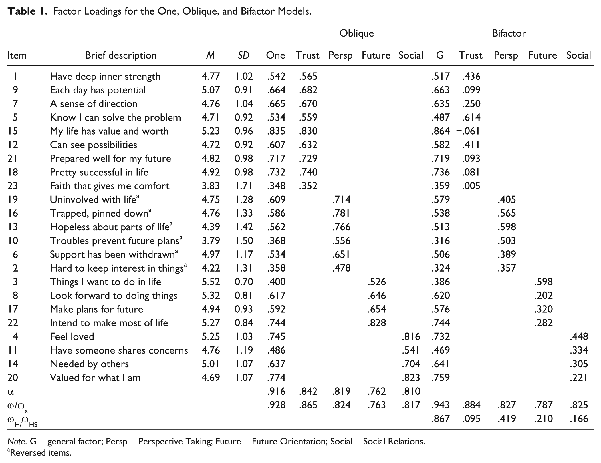
Note. G = general factor; Persp = Perspective Taking; Future = Future Orientation; Social = Social Relations.
Reversed items.
Model Fit for the One, Oblique, Higher Order, and Bifactor Models.

Note. df = degrees of freedom; CFI = Comparative Fit Index; RMSEA = Root Mean Square Error of Approximation; AIC = Akaike Information Criterion; BIC = Bayesian Information Criterion.
Turning to Table 2, fit for the one-factor model was clearly unacceptable (i.e., CFI = .775; RMSEA = .103) and far worse than for the oblique factor model which had marginally acceptable fit (i.e., CFI = .874; RMSEA = .078). Values for AIC and BIC supported the superiority of the oblique factor model over the one-factor model as did a chi-square difference test, Δχ2(6) = 317.814, p < .001. Tabachnick and Fidell (2007) regard factors correlated less than r = .33 to be essentially uncorrelated. On that basis, correlations between the four factors in the oblique factor model were substantial (p < .001). From smallest to largest correlations, r(286) = .557 for Lack of Perspective and Future Orientation, r(286) = .683 between Lack of Perspective and Social Relations, r(286) = .694 between Trust and Lack of Perspective, r(286) = .754 between Future Orientation and Social Relations, r(286) = .882 between Trust and Social Relations, and r(286) = .924 between Trust and Future Orientation.
Omega (ω) values were comparable to Cronbach’s alpha for the one-factor and oblique factor models. Cronbach’s alpha for the items in the one-factor model was α = .916; Omega was .928. Gignac and Watkins (2013) suggest a difference of .06 or more between Cronbach’s alpha and Omega is a substantial difference. Cronbach’s alpha for the subscales and OmegaS (ωS) subscale values were also similar in size (see Table 1).
In order to allow an admissible solution for testing the higher order factor model, it was necessary to constrain the variance for the Trust factor to a small value (.05). Model fit for the higher order factor model was indistinguishable from fit for the oblique factor model. The general factor accounted for 76.2% of the explained variance; the subscale factors explained 23.8% of explained variance. Looking at the Schmid–Leiman transformed factor loadings for the higher order factor model (Table 3), all Lack of Perspective subscale items had factor loadings above .30, Thurstone’s (1947) cutoff for factor loading salience, as did three of the Social Relations subscale items. None of the Trust subscale items and only one of the Future Orientation subscale items met Thurstone’s criteria for factor loading salience. Furthermore, all of the items of the Lack of Perspective subscale factor had higher loadings on the subscale factor than on the higher order general factor.
Factor Loadings for the Higher Order Model Following Schmid–Leiman Transformation.

Note. Persp = Perspective Taking; Future = Future Orientation; Social = Social Relations.
Turning again to Table 2, the best fitting model was the bifactor model. In order for the bifactor model to be identified, one item associated with the higher order general factor was set to one, and one item from each subscale factor was set to one (Chen, West, & Sousa, 2006). Compared with the other factor models, the bifactor model had the smallest chi-square value, the largest CFI value, the smallest RMSEA value, and the smallest AIC and BIC values, all of which indicate comparative good fit. The bifactor model can be compared directly with the higher order factor model using a chi-square difference test (Brunner et al., 2012). Doing so found the bifactor model fit the data better than the higher order factor model, Δχ2(20) = 141.103, p < .001.
Having found the bifactor model to be the best fitting model, we compared OmegaH with Omega for the bifactor model (Table 1). The ratio of .867 to .943 indicates that 92% of reliable variance is due to the general factor. As a point of comparison, Rodriguez et al. (2016a) in a review of 50 recent bifactor model estimation studies found the mean OmegaH estimate to be .80 (SD = .10) and the mean Omega estimate to be .94 (SD = .03), a difference of .14 higher for Omega. Thus, the IHS general factor again is shown to account for a substantial proportion of the reliable variance in comparison with the subscale factors in the bifactor model.
The OmegaS (ωS) and OmegaHS (ωHS) statistics are also reported in Table 1. Consider for example the OmegaS statistic for Trust of .884. This value implies 88.4% of the variance in Trust scores is the product of the combination of the higher order general hope factor and the Trust subscale factor. In contrast, OmegaHS for Trust of .095 implies that only 9.5% of the variance in the Trust subscale is attributable to Trust, per se. In the Rodriguez et al. (2016a) review of 50 bifactor model estimations, the mean OmegaHS was what they called a “meager .27 (SD = .17) suggesting that most of the subscales in this set provide little unique, reliable variance” (p. 225). One exception to this result for the IHS is for Lack of Perspective. For that subscale, a substantial percentage (41.9%) of subscale score variance is attributable to that subscale and not to the general hope factor. Again, these results support the argument that this subscale is reflective of hopelessness not hope, thereby not contributing to the general hope factor like the other subscales.
As a test of dimensionality, ECV was calculated for the bifactor model by summing the squared loadings for the general factor and dividing that value by the sum of the squared loadings for the general and subscale factors. ECV was .715, implying the general factor accounted for the majority of common variance, supporting a unidimensional model. While there are no benchmarks for ECV (Reise, 2012), the mean ECV reported by Rodriguez et al. (2016a) in their summary of estimating 50 bifactor models was .67 (SD = .10).
Table 4 presents the correlations between the IHS total and subscale scores, and measures of time perspective (the ZTPI), hedonic well-being (the PANAS and the TSWLS), and eudaimonic well-being (the MAP). As anticipated, the IHS total and subscale scores were correlated positively with positive affect, satisfaction with one’s life (past, present, and future), and self-actualization, and correlated negatively with negative affect.
Correlations Between the IHS and Measures of Other Constructs.

Note. IHS = Integrative Hope Scale; Persp = Perspective Taking; Future = Future Orientation; Social = Social Relations; ZTPI = Zimbardo Time Perspective Inventory; PANAS = Positive and Negative Affect Schedule; TSWLS = Temporal Satisfaction With Life Scale; MAP = Measure of Actualization of Potential.
p < .01. **p < .001.
With regard to time orientation, seeing the past positively was associated positively with all dimensions of hope, while seeing the past negatively was associated negatively with all dimensions of hope. Similarly, seeing the present in fatalistic terms was negatively associated with all dimensions of hope. The relationship between hope and a present-hedonistic time orientation was more complex. A present-hedonistic orientation was not associated with the IHS total score, but was associated positively with the Trust subscale and Future Orientation subscale of the IHS. Finally, having a future time orientation was only modestly related, albeit positively, to the IHS total score and, not surprisingly, the Future Orientation subscale of the IHS.
A canonical correlation analysis was conducted to explore the complexity of the relationships between the subscales of the IHS and the ZTPI. The results from the canonical correlation analysis were consistent with the findings from the correlation matrix reported in Table 4. The relationship between the two sets of subscales was statistically significant, Wilks’s lambda = .40, R2c = .60, F(20, 926.29) = 14.67, p < .001. The first function (eigenvalue = 1.13, R2c = .53) accounted for 87.23% of the explained variance. The second function (eigenvalue = .14, R2c = .12) accounted for an additional 10.75% of the explained variance. The first two functions were statistically significant (p < .001); the remaining two functions were not. Interpreting the structure coefficients for the first function suggested that for the ZTPI high scores on Past Negative (r = .87) and Present Fatalistic (r = .58), and low scores on Past Positive (r = −.62), were associated with low scores on all four subscales of the IHS (r = −.81 for Trust, r = −.92 for Lack of Perspective, r = −.69 for Future Orientation, r = −.70 for Social Relations). For the second function, low scores on the ZTPI Present Hedonic (r = −.79) were associated with low scores on IHS Future Orientation (r = −.69).
Discussion
Confirmatory factor analysis found the one-factor unidimensional model to be a poor fit to the IHS data. Computing a total score for a measure assumes that the items of a scale are unidimensional (Brown, Finney, & France, 2011). However, unidimensionality is not always desirable. Gustafsson and Aberg-Bengtsson (2010) suggest that requiring a measure to be unidimensional may lead to a narrow construct focus and can be misleading given multidimensional constructs are the norm.
Indeed, a much better fit was found for multidimensional models of the IHS, specifically the bifactor model, but also the oblique and higher order models. An oblique factor model has each item load on correlated factors representing the subscales of a measure. However, an oblique factor model is not a measurement model, per se. Unlike higher order and bifactor models, an oblique factor model contains no general hope factor, no “one common target dimension to be measured or that directly affects item variance” (Reise et al., 2010, p. 546).
There was much support in the present study for a strong general hope factor that captures common variance across items. First, model fit was best for the bifactor model, which includes a higher order general factor. Second, a general factor explained a considerable amount of variance in both the higher order model and the bifactor model. Third, a general factor also accounted for a substantial proportion of the common variance according to calculation of the ECV statistic.
At first glance, the finding for a strong general factor might seem inconsistent with the failure to find a well-fitting unidimensional model. However, according to Reise et al. (2010), “It is unsurprising that in many psychometric investigations, it is common to observe evidence for a single dimension [the general factor] and at the same time to uncover evidence of multidimensionality” (p. 544). Indeed, Rodriguez et al. (2016a) in their review of 50 bifactor models from the literature found almost all those bifactor models were associated with multidimensionality but also a strong general factor. Reise et al. (2010) argue this dimensionality issue arises because while the authors of measures of psychological constructs frequently write scale items with a unitary construct in mind, many psychological constructs are not unitary. From Snyder’s (1995) perspective, for example, hope is a striving toward accomplishing one’s life objectives. However, striving to accomplish one’s life objectives can take many forms, and there can be many varied, and frequently contradictory, objectives in one’s life. In that vein, Dufault and Martocchio’s (1985) seminal multidimensional model of hope implies hope can be understood as a both/and construct in that hope can be both a generalized experience and directed to particularized events or outcomes.
In the circumstances of a strong general factor in the presence of multidimensionality, it is appropriate to compute and interpret the total scale score. Again turning to Rodriguez et al.’s (2016a) review of 50 bifactor models, “unit-weighted total scores . . . can be interpreted as univocal indicators of a single latent variable, despite the [presence of] multidimensionality” (p. 232). One example from the literature is Brewster et al. (2016) who evaluated the Measure of Atheist Discrimination Experiences (MADE). Similar to our review of the IHS, Brewster et al. (2016) found support for a multidimensional atheist discrimination construct and yet reported a strong general factor that accounted for much of the variance in subscale scores. Their conclusion was “model-based reliability analyses provided support for the use of the MADE total scores to represent [the] general discrimination construct” (pp. 563-564, italics added).
Brewster et al. (2016) found little variance was accounted for by subscale scores of the MADE. Similarly, our examination of the IHS suggested little variance was explained by the subscale factors of the IHS with the exception of Lack of Perspective. This subscale distinguished itself from the general factor in both models, specifically the highest factor loadings after a Schmid–Leman transformation in the higher order factor model, and a substantial OmegaHS value in the bifactor model. This outcome may be a result of the Lack of Perspective subscale measuring the theoretically distinct construct of hopelessness, instead of its intended target of hope. Unfortunately, there is an inherent confound in the Lack of Perspective subscale; all of the items are negatively keyed. Thus, it is not clear whether the Lack of Perspective subscale factor has substantive merit or if it merely reflects a method factor (Gignac, 2007). Indeed, it could be both; it is possible that a subscale factor is a substantive factor and also a negatively keyed item method factor (Gignac et al., 2007). While it is important researchers constructing a scale include negatively keyed items to avoid an acquiescent response set, it is unfortunate that the content of all reverse coded items in the IHS pertains to the same psychological dimension, what Miller and Powers (1988) called an avoidance of hope threats.
While the subscales of the IHS accounted for little substantive variability according to our calculation of OmegaHS statistics, that is not to say the subscales made no contribution to understanding the validity of the IHS. Although this study was focused primarily on issues of reliability and factor structure of the IHS, it was also important to document that the IHS has predictive validity. Factor structure has little meaning if a scale is unrelated to other constructs in a theoretically appropriate manner. IHS scale and subscale scores were associated with past time orientations, both positive and negative, and present-fatalistic time orientation. A future time orientation was also associated with hope, albeit only for the total IHS scale and the Future Orientation IHS subscale. Why was a future time orientation not more strongly related to hope given that the hope literature (e.g., Scioli et al., 2011) implies a future orientation is of utmost importance in the hoping process? This appears puzzling, but only momentarily. Being oriented toward the future is important but the future is always hypothetical, in some sense an empty canvas onto which we project what we sense is possible. What we sense is possible is derived primarily from the past, from how we interpret and assimilate everything that has happened to us thus far in our lives. A powerful example of what this means in practical terms is given in Snyder, Rand, and Ritschel (2006), who suggest that hope is dispositional, arising from past experiences of achieving (or failing to achieve) goals in infancy and childhood. Early successes with overcoming obstacles teach the young child problem-solving skills and resilience; early failures lead to expectations of defeat and feelings of discouragement. These findings suggest that reflections on past experiences may be the most important time relevant correlates to hope.
One additional finding pertaining to subscales of the ZTPI and IHS was that a present hedonistic time orientation as measured by the ZTPI was associated positively with the Future Orientation and Trust subscales of the IHS but not the total score of the IHS. This lack of association to the total IHS score is not as surprising as it might seem at first glance; in fact, it serves to underline the practical and conceptual value of recognizing that the IHS is a multidimensional scale even if generally dominated by one factor. In this instance, there is a small, positive but statistically nonsignificant correlation between present hedonistic time orientation and the overall IHS scale, but two small and statistically significant positive correlations with subscales of the IHS. The present hedonistic mind-set is characterized by a focus on novelty seeking and sensation seeking (Zimbardo & Boyd, 1999), which is a positive view of the immediate future but one that is severely constrained and blinkered. Present hedonism is an attitude that indicates a complete unwillingness to postpone seeking the rewards of more superficial immediate pleasures for the sake of larger or more meaningful future benefits. This larger, more deeply expansive engagement with a hopeful future is perhaps what the overall IHS would signify, but there is still an engagement with smaller but real aspects of hope as represented by the two subscales of Trust and Future Orientation. These two dimensions, as cut off from the whole construct of hope, would seem to mean having the necessary self-confidence and orientation to the very immediate future to believe that these more sensation-seeking pleasures are possible. This is a very good practical example of how the total IHS score can and should be used to measure a large, unitary construct but that the subscales should always be examined and can occasionally be of real interpretive use.
Finally, hope as measured by the IHS was associated in anticipated ways with hedonic well-being, specifically positive and negative affect and life satisfaction, and with eudaimonic well-being, specifically self-actualization. Hedonic well-being in this context should not be confused with present hedonism, which is an orientation toward time focused on pleasure in the present moment. Hedonic well-being denotes a joyful, upbeat attitude toward a generally satisfying life (Waterman, 1993). Eudaimonic well-being is a more existential concept which does not principally refer to any type of pleasure or satisfaction, but rather to an awareness of, and commitment to, one’s purpose and meaning in life (again, see Waterman, 1993). It is the happiness and well-being that flow from choosing to live with integrity from one’s deepest values. These are distinct approaches to well-being that can occasionally come into conflict but they are both concerned with aspects of the complex array of human goods that are indicated by the multidimensional construct of hope. It was fully expected that they would both be predicted by the IHS and that is what we found.
One strength of the present study was our use of a North American community sample. Many previous studies that have employed the IHS have used European samples, requiring the measure to be translated into other languages (most frequently German), and specialized samples (e.g., caregivers of cancer patients, individuals in treatment for psychosis). Other strengths of the present study were our use of the bifactor model and our calculation of Omega statistics. The best fitting model was the bifactor model. In one sense that outcome is not surprising; a bifactor model will almost always be a better fit than oblique or higher order factor models because those models are nested within the bifactor model (Reise et al., 2013). The use of bifactor models to assess the dimensionality and reliability of a measure is controversial. Bifactor models have been “poorly received by personality, psychopathology, and health outcomes researchers” (Reise et al., 2010, p. 557). Reise et al. (2010) attributed this lack of acceptance of bifactor models to the absence of options to calculate bifactor model in statistical packages such as SPSS, but also because of issues with their interpretation, model specification, and assumptions. Bagby, Taylor, Quilty, and Parker (2007) suggested the superior fit of bifactor models can be attributed to the adding of parameters to a model, thereby overfitting the model and artificially improving model fit. While extolling the virtues of bifactor models for their psychometric insights (e.g., calculating Omega statistics), Bonifay, Lane, and Reise (2017) suggest caution in concluding a bifactor model is the best representation of a psychological construct.
Omega statistics have been infrequently employed by researchers to date (Gignac & Watkins, 2013). To calculate Omega statistics, one requires factor loadings from a factor analysis; Cronbach’s alpha requires only raw data. Omega statistics are also not available in standard software packages such as SPSS, while Cronbach’s alpha is readily obtained. Omega statistics are more challenging to interpret than Cronbach’s alpha. For example, reliability for subscales is underestimated by OmegaHS values because the variance accounted for by the general factor has been removed (Rodriguez et al., 2016a). However, given the clear and widely acknowledged limitations to Cronbach’s alpha, the popularity of Omega coefficients should increase if it can be shown that there are substantial differences in the results from Cronbach’s alpha and Omega statistics.
In conclusion, we recommend researchers continue to utilize total IHS scale scores. The IHS showed a strong general hope factor and was found to be a reliable measure in our sample. However, IHS subscale scores, especially for the Lack of Perspective subscale, also should be reported. In that regard, there needs to be further research to determine whether the Lack of Perspective subscale reflects a substantive construct, perhaps hopelessness, or a method bias arising from the clustering of negatively worded items. Given the importance of hope to psychological well-being, further investigations need to be made into the nature of hope as measured by the IHS and other related scales.
Footnotes
Declaration of Conflicting Interests
The author(s) declared no potential conflicts of interest with respect to the research, authorship, and/or publication of this article.
Funding
The author(s) received no financial support for the research, authorship, and/or publication of this article.