When Does Differential Item Functioning Matter for Screening? A Method for Empirical Evaluation

Abstract

When items in a screening measure exhibit differential item functioning (DIF) across groups (e.g., males vs. females), DIF might affect which individuals are “caught” in the screening. This phenomenon is common, but DIF detection procedures do not typically provide guidance on whether the presence of DIF will meaningfully affect screening accuracy. Millsap and Kwok proposed a method to quantify the impact of DIF on screening accuracy, but their approach had limitations that prevent its use in scenarios where items are discrete. We extend the Millsap and Kwok procedure to accommodate discrete items and provide R functions to apply the procedure to the user’s own data. We illustrate our approach using published screening information and evaluate the proposed methodology with a small simulation study. Overall, we encourage researchers to use empirical methods to evaluate the extent to which the presence of DIF in a screening measure materially affects screening performance.

Keywords

screener differential item functioning impact item response theory measurement bias sensitivity specificity

Screening measures are used to improve the efficiency of clinical assessment. The screening measure is typically briefer, cheaper, and less burdensome than the full assessment. For example, suppose that a health care network is screening all adults in primary care for major depressive disorder (MDD). Only 6.6% of adults meet Diagnostic and Statistical Manual of Mental Disorders criteria for MDD (Kessler et al., 2003), so administering a full diagnostic interview to every patient in the network would expend a large amount of the time of both providers and patients. A more efficient approach is to first administer a low-burden screening measure, then complete a full diagnostic interview only with those individuals who are flagged by the screening. When screening for MDD, a common approach is to administer the Center for Epidemiologic Studies of Depression (CES-D) Scale and follow-up with respondents who obtain total scores greater than or equal to 16 (Vilagut et al., 2016). In almost all cases, the screening measure consists of a series of binary items (i.e., a symptom is present or not) or polytomous items (i.e., Likert-type scale), and item responses are counted or totaled to estimate an observed score. The assessor then classifies the respondent by comparing the observed score with a predetermined cutscore (Youngstrom, 2013) or a percentile of risk (e.g., Lochman & The Conduct Problems Prevention Research Group, 1995).

When completing a screening measure, respondents from a target group may systematically rate themselves higher or lower on items than a different group. This is referred to as measurement bias or differential item functioning (DIF). For example, previous research suggests that Latinos are more likely than non-Latinos to endorse items from the Beck Depression Inventory (Beck et al., 1961) related to crying even when they are equivalent in level of depression. Latinos may be more willing to endorse these items because crying is more socially acceptable in Latino cultures (Azocar et al., 2001). Score differences on these items therefore represent culture-based differences in the pattern of responding rather than true differences in the construct of interest—depression. As a result of this overendorsement, Latinos will have greater observed scores for depression than non-Latinos even when their true level of depression is identical. In this case, the crying items exhibit DIF across groups (Millsap, 2011).

In the context of a screening measure, the presence of measurement bias is troubling. The goal of screening is to identify those at the highest levels of the construct of interest (e.g., depression), not to identify those from groups for whom there is positive bias on the screening measure. Ignoring measurement bias could lead respondents from a certain group to be more likely “caught” in the screening. Similarly, measurement bias could lead respondents from a different group to be less likely “caught” in the screening. Last, there could be situations in which measurement bias in the assessment does not affect screening performance across groups. Returning to our earlier example, suppose that the CES-D is being used to screen adults in a primary care network for MDD and those with a CES-D total score greater than or equal to 16 are flagged for a complete diagnostic assessment. The systematic overendorsement of crying items may place a disproportionate number of Latino adults over the CES-D cutscore, even though their true level of depression is lower than non-Latinos who are not flagged for a diagnostic interview. Screening based on the CES-D total score would produce more false positives among Latinos, yielding lower sensitivity. The same would be true if a percentile were used (e.g., top 10%) instead of a predetermined cutscore.

Standard approaches to testing for DIF focus on the statistical question of whether the relation of an item to the construct of interest varies across groups (Millsap, 2011; Teresi et al., 2006). These methods typically do not provide guidance on whether the bias materially affects the performance of the measure in a screening context, even though this is often of practical importance. In other words, DIF testing consists on testing for statistical significance in item bias, rather than assessing if the item bias is practically significant (Lai et al., 2017; Lai et al., 2019). Recently, effect sizes to estimate the magnitude of DIF have been discussed (Kleinman & Teresi, 2016; Meade, 2010), but most are associated with differences in expected scores or differences across parameters per group, not with screening (Lai et al., 2019; Millsap & Kwok, 2004). In our running example, even though significance testing might flag several CES-D items as having DIF in Latinos versus non-Latinos, this does not necessarily imply that DIF will lead to worse sensitivity or specificity in the measure. If Latinos overendorse the crying items and also underendorse a different subset of items, this might not convey worse screening performance, so the assessor may safely continue to use that measure. This situation is referred to as DIF cancellation (Chalmers et al., 2016). On the other hand, if the screener exhibits DIF that does convey worse screening performance, then the assessor may need to drop the items that exhibit DIF or stop using the screener. Thus, there is need for methods to empirically evaluate how the presence of DIF on a measure affects screening performance.

The purpose of this article is to extend earlier work evaluating the impact of measurement bias on screening (Lai et al., 2017; Lai et al., 2019; Millsap & Kwok, 2004) to a more general class of clinical assessment scenarios. We focus on extending the methodology developed by Millsap and Kwok (2004), one of the few approaches that describes the effect of DIF at the aggregate level of a measure whose end goal is selection—the screening process is inherently a selection problem. First, we review item response theory (IRT) models that analyze measures with discrete item responses and test for DIF. Second, we describe the approach by Millsap and Kwok (2004) to evaluate the impact of measurement bias and identify key limitations. Finally, we introduce extensions of their method that improve its utility in real-world screening scenarios and use simulations and illustrations to evaluate our proposed methodology.

Item Response Theory Models

The methods in this article are based on IRT, a family of latent variable models that allow for a detailed analysis of items with discrete responses (Edelen & Reeve, 2007; Thissen & Wainer, 2001; Thomas, 2011). A widely used item response model that describes the probability of endorsing Likert-type item responses is the graded response model (GRM; Samejima, 1969), expressed as follows:

\begin{array}{l} T (u_{i} = k | θ) = \frac{1}{1 + \exp (- a_{i} (θ - b_{i (k)}))} \\ - \frac{1}{1 + \exp (- a (θ - b_{i (k + 1)}))} \\ = T^{*} (k) - T^{*} (k + 1) . \end{array}

(1)

In this case, u refers to the observed value when the respondent endorses category k on item i, the θ parameter refers to the respondent’s standing on the underlying construct that the items measure, the a-parameter refers to the relationship between item i and the construct (analogous to a factor loading in factor analysis), and the b-parameters indicate the location in the range of θ where respondents have a 50% probability of endorsing category k or a higher category. If the item is comprised of m categories, then there would be m − 1 b-parameters. The $T^{*} (k)$ represents the trace line that describes the probability of responding k to item i or higher. Also, by model definition, $T^{*} (0) = 1$ and $T^{*} (k_{m} + 1) = 0$ , where $k_{m}$ is the highest category. If the item is only comprised of two categories, then the GRM reduces to the two-parameter logistic (2PL) model, which is a widely used item response model for binary items (with symbols defined above):

T (u_{i} = k | θ) = T (u_{i} = 1 | θ) = \frac{1}{1 + \exp (- a_{i} (θ - b_{i}))} .

(2)

The models in Equation 1 or Equation 2 can be used to produce trace lines (see Figure 1), which show the relation between a respondent’s standing on the latent variable and his or her probability of endorsing a specific item category for a specific item. For a binary item (Figure 1A), the 2PL trace line shows that the predicted probability of endorsing the item increases as θ increases. For a polytomous item (Figure 1B), the GRM trace lines show that the probability of endorsing a higher item category increases as θ increases.

Figure 1.

Item response trace lines showing the relationship between the construct and the probability of endorsing a response option: (A) Trace line for a single item in the 2PL model; (B) Trace lines for a single item in the graded response model; (C) Trace lines for a single item in the 2PL model exhibiting DIF across Latinos (dashed line) and non-Latinos (solid line); (D) Trace lines for a single item in the graded response model exhibiting DIF across Latinos (dashed lines) and non-Latinos (solid lines).

Certain assumptions must hold for item response models to give accurate results (Thissen & Wainer, 2001). First, we assume that the correct number of latent variables has been specified in the item response model. Second, we assume local independence, or that item responses are unrelated, conditional on the latent variable(s). Third, we assume that the item parameters—and thus the trace lines—are the same across groups. Figure 1C and Figure 1D illustrate the case in which this assumption is violated: at the same value on the latent variable, Latino and non-Latino respondents have different predicted probabilities of endorsing an item response. The measurement is not invariant across the groups. Rather, these two items exhibit DIF and introduce measurement bias to the assessment (Edelen & Reeve, 2007). Our proposed procedure requires that researchers meet the first two assumptions (i.e., unidimensionality and local independence) and evaluates how screening decisions change when the third assumption (measurement invariance) is not met.

Measurement Invariance and Differential Item Functioning

The presence of DIF indicates a lack of measurement invariance. Measurement invariance is required to compare observed scores between two groups (Meredith, 1993). If measurement invariance is violated, then observed differences between two groups could be due to (a) true differences in the latent construct, (b) systematic bias in measurement, or (c) the combination of (a) and (b). Both (b) and (c) can lead to incorrect inferences about observed group differences, the construct, or its relation to other criteria. Methodologists have developed many different procedures to test if items exhibit DIF (Millsap, 2011; Teresi et al., 2006; Thissen et al., 1993). If some items have been flagged with DIF, it is important to evaluate the impact of DIF on the decisions based on the respondent’s score on the overall measure. As described earlier, DIF may positively or negatively bias overall observed scores from a specific group of respondents (e.g., Latinos), which may in turn affect the sensitivity or specificity of the screening procedures based on the observed scores. However, DIF may be statistically detectable yet have no practical impact on screening performance. Below, we describe the Millsap and Kwok (2004) procedure to empirically evaluate the degree to which the presence of DIF on a screening measure affects the sensitivity and specificity of the screening procedure.

Evaluating the Impact of Differential Item Functioning on Screening Performance

Suppose that the assessor is interested in using a unidimensional measure to screen for depression in order to identify participants high on the depression construct. In theory, if a model in which partial invariance (e.g., some but not all items exhibit DIF) is confirmed and latent variable scores for depression were known, these latent variable scores would be used for screening because they would not be influenced by measurement bias (Teresi et al., 2012). However, screening is usually based on the observed score (e.g., summed score on the CES-D), which is an imperfect estimate of the latent variable score that is prone to measurement bias.

As shown in Equation 1 and Equation 2, item response models assume that there is a relation between the latent variable score and the probability of endorsing an item category. Millsap and Kwok (2004) used this property to develop an analytical procedure to evaluate the impact of DIF on screening performance. Their procedure studies the agreement between classifying respondents using the latent variable and classifying respondents using observed scores across two conditions. Given a set of latent variable scores, one first derives the expected observed scores from an IRT model where DIF is present ( $M_{d i f}$ ; items with DIF have group-specific item parameters). Then, given the same set of latent variable scores, one derives the expected observed scores from an IRT model where DIF is ignored ( $M_{i n v}$ ; items with DIF have the same item parameters across groups). For each group, we compare the classification agreement of the latent variable with (a) the classification of the expected observed scores under $M_{i n v}$ and with (b) the classification of the expected observe scores under $M_{d i f}$ . Two indices of agreement are sensitivity and specificity. Sensitivity would be the number of cases above the cutscore on the latent variable whose expected observed score under $M_{d i f}$ is above the observed cutscore, and specificity would be the number of cases below the cutscore on the latent variable whose expected observed score under $M_{d i f}$ is below the observed cutscore (note that sensitivity and specificity could also be calculated relative to the expected observed scores under $M_{i n v}$ ). The difference in classification agreement under $M_{i n v}$ versus $M_{d i f}$ is an index of the impact of measurement bias on screening performance. A major advantage of the Millsap and Kwok (2004) procedure over other DIF effect sizes is that it describes the impact of DIF in terms that are familiar to assessment specialists, such as differences in sensitivity and specificity. By considering differences on these practical metrics, assessment specialists can make more informed decisions about screener use in a specific substantive application.

However, the Millsap and Kwok (2004) procedure has a key limitation: it assumes that item responses are continuous and normally distributed. This restricts its use in realistic assessment scenarios because many questionnaire-based screening measures consist of items with just a few response options. This limitation has been partially addressed by Lai et al. (2019), who used an analytical approach to extend the Millsap and Kwok (2004) method to the case of scales with binary (i.e., yes/no) items. However, analytical methods for polytomous (Likert-type) items (e.g., never/sometimes/always) have not been developed, perhaps because it is analytically difficult to derive the relation between the observed score and the latent variable in that scenario (Millsap, 2013).

Present Study

In this article, we propose a simulation-based method that allows the investigator to quantify the impact of DIF on screening performance with either binary or polytomous items, generalizing the Millsap and Kwok (2004) method to a broader class of potential applications. The proposed method describes the magnitude of DIF in a language familiar to assessment specialists, empirically evaluates whether the presence of DIF on a screening measure affects screening performance, and handles binary and polytomous items that comprise most screeners. Our approach extends the Millsap and Kwok (2004) procedure by incorporating IRT models to acknowledge the discrete nature of items and by using Monte Carlo simulation methods to approximate the relation between observed scores and latent variable scores (as opposed to deriving the relation between observed scores and latent variable scores analytically; Lai et al., 2019; Millsap, 2013; Millsap & Kwok, 2004). First, we describe the proposed procedure. Second, we illustrate our procedure using information from a published DIF study on CES-D scale across mode of assessment (Chan et al., 2004). Third, we report results from a simulation study that compares the simulation-based methods to the existing analytical method by Lai et al. (2019) in the context in which they both can be applied (i.e., binary items) and evaluate how many iterations of simulation are needed to provide stable estimates of screening performance. In the supplement (available online), we provide a suite of R functions for users to apply the simulation-based procedure method in their own data and a step-by-step tutorial on how to do so. For simplicity, our procedure assumes that the screening measures fit a unidimensional model and that a subset of the items has been accurately flagged with DIF.

Description of Proposed Method

General Procedure for the Proposed Methodology

The proposed procedure is simulation-based and takes a few seconds to complete on a MacBook Pro with 3.1 GHz and 16 GB of RAM. Below, we outline the general procedure. The supplementary materials (available online) present R functions to implement the procedure. To use the functions, the end user needs only to specify three pieces of information commonly found in any DIF study: (a) mean and variances of the latent variable per group, (b) item parameters per group, where the parameters of DIF-free items are constrained to equality across groups, and (c) the proportion of cases belonging to each group. Raw data are not needed unless the DIF study is yet to be carried out.

Suppose that one suspects that there is DIF across gender. Our R functions automate the following steps:

Simulate latent variable scores for large number of respondents (N = 25,000). Specifically, a latent variable score for a male would be a draw from a normal distribution with mean µ_M and variance $σ_{M}^{2}$ . On the other hand, a latent variable score for a female would be a draw from a normal distribution with mean µ_F and variance $σ_{F}^{2}$ . Match the proportion of cases of males versus females to population proportions (i.e., 50% to 50%). In applications where the population proportions are not known, match the number of cases to the sample proportions in the study (e.g., if the sample was 75% female, then 75% of the simulated respondents should be female).

For each case, simulate an item response pattern by inputting the respondent’s latent variable score to an item response model that accounts for DIF ( $M_{d i f}$ ; males and females have some item parameters that are the same and some that are allowed to differ). For each case, sum the item responses to calculate the observed score under $M_{d i f}$ .

Choose a pair of cutscores in (a) the latent variable score and the (b) observed score under $M_{d i f}$ that each separate the same proportion of the distribution. For example, suppose the screening procedure typically flags those with observed scores greater than 10. Fix the cutscore in the distribution of observed scores at 10. Calculate the proportion of cases at or above this cutscore. Then, find the latent variable score above which there is the same proportion of cases. Fix the cutscore in the distribution of the simulated latent variable scores to be this calculated value.

Calculate classification accuracy for the 2 × 2 table defined by being above/below the cutscores in the latent variable and observed score under $M_{d i f}$ . These statistics indicate screening performance under a model that accounts for DIF.

Repeat Step 2, but now for each case, simulate an item response pattern by inputting the respondent’s latent variable score to an item response model that ignores DIF ( $M_{i n v}$ ; all item parameters are the same across males and females). For each case, sum the item responses to calculate the observed score under $M_{i n v}$ .

Calculate classification accuracy for the 2 × 2 table defined by being above/below the cutscores (same values from Step 3) in the latent variable and observed score under $M_{i n v}$ . These statistics indicate screening performance under a model that ignores DIF.

Compare the estimates of screening performance obtained in Step 4 and Step 6 per group. Evaluate the magnitude of any differences in light of the specific assessment application.

Screening Performance

Performance Metrics

Steps 4 and 6 above referred to classification accuracy as the measure of screening performance. However, many statistics can be calculated from a 2 × 2 table, including sensitivity, specificity, positive predictive value, or negative predictive value (Youngstrom, 2013). Table 1 illustrates calculations for several statistics that can be used to characterize screening performance under models that ignore versus account for DIF.

Table 1.

2 × 2 Contingency Table to Estimate Classification Performance.

		Observed score
	Latent variable score	Below cutscore	Above cutscore
	Below cutscore	TN	FP
	Above cutscore	FN	TP
Sensitivity = TP / (TP + FN)Specificity = TN / (TN + FP)Classification rate = (TP + TN) / (TP + TN + FP + FN)Proportion identified = TP + FP

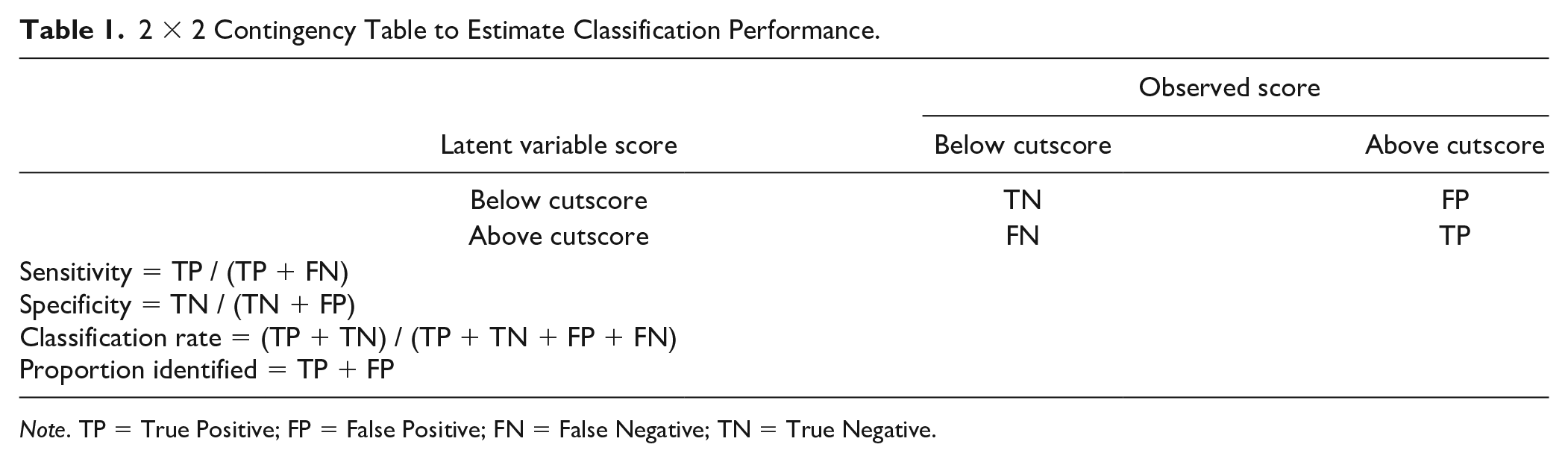
Note. TP = True Positive; FP = False Positive; FN = False Negative; TN = True Negative.

Multiple-Cutscore Scenario

Step 3 above referred to choosing a single cutscore in the latent variable score and a single cutscore in the expected observed score. However, the choice of cutscore might vary as a function of the resources available or assessment goals. For example, if an intervention is cheap, a low cutscore would prevent researchers from missing respondents with the condition, and if an intervention is expensive and invasive, a high cutscore would guarantee that respondents who receive the intervention actually needed it. For example, although an observed score ≥16 is a common cutscore used when screening with the CES-D, a cutscore of >20 is also often used (Vilagut et al., 2016). Thus, it would be important to evaluate the impact of DIF when screening at multiple cutoffs. To do so, Steps 4 and 6 can be repeated using different cutscores, or even across the range of cutscores. Considering a range of all possible cutscores might be especially important when a measure does not have a recommended cutscore, but rather is used to identify a fixed proportion of those most at risk (e.g., the upper 30%, 20%, or 10%).

Application of Proposed Method

This section illustrates the proposed methodology in a specific application. An additional fully worked example using the R functions we have written is included in the supplement (available online).

CES-D and DIF by Mode of Assessment

The CES-D, originally developed to be administered in a face-to-face interview, is composed of 20 four-category items that assess different aspects of depression, such as depressed and positive affect, somatic and retarded activity, and interpersonal aspects of depression (Radloff, 1977). Item parameters were obtained from the DIF study by Chan et al. (2004; see Table 3 of original article) on the CES-D across mode of assessment. The authors suggest that there might be measurement bias when the CES-D is administered through the phone (n= 139) or through mail (n = 139) in a primary care population. To identify the model, Chan et al. (2004) specified that the mean and variance of the latent variable equaled 0 and 1, respectively, for both groups. Also, the authors indicated which items were flagged with DIF, but they did not constrain DIF-free item parameters to be the same across groups. For an item parameter that was not flagged with DIF, we estimated a hypothetical invariant parameter by taking a weighted average of the item parameter across both groups. The authors determined that the CES-D items were unidimensional, and that 12 out of the 20 CES-D items exhibited measurement bias across mail and phone respondents. Item parameters suggest that mail respondents were more likely to endorse depression items than phone respondents, with up to a 13% increase in probable depression in the mail respondents, independent of the items’ stigma as rated by content experts (Chan et al., 2004). We now use the proposed simulation approach (with steps outlined above) to study how measurement bias across mode of assessment affects the sensitivity and specificity of the CES-D in screening for depression.

Using 25,000 simulated cases per group, the relationship between the simulated CES-D theta score and the estimated CES-D observed score under the model that allows for DIF is presented in Figure 2. We evaluated screening performance of the recommended CES-D cutscore of greater than or equal to 16, which indicates possible MDD. In the mixed distribution of phone and mail respondent summed scores, the recommended CES-D cutscore identified the top 50.6% of respondents. In the mixed distribution of phone and mail respondents’ theta scores, a cutscore greater than or equal to 0.022 identified the same proportion (50.6%) of respondents.

Figure 2.

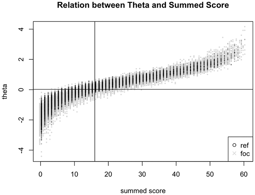
Relationship between the CES-D theta score and the CES-D summed score (black: phone respondents, gray: mail respondents).

Based on these cutscores, we calculated assessment sensitivity, specificity, and other classification statistics (see Table 2). If measurement invariance were to hold, the sensitivity of the measure for mail and phone respondents would be 0.94. However, given that measurement invariance did not hold (i.e., some items exhibit DIF), the sensitivity of the measure was 0.98 for mail respondents and 0.88 for phone respondents. Therefore, DIF in the measure led to a lower likelihood of identifying depressed respondents by phone than over the mail. If measurement invariance were to hold, the specificity of the measure for mail and phone respondents would be 0.93. Given that measurement invariance did not hold, the specificity of the measure was 0.87 for mail respondents and 0.97 for phone respondents. Therefore, DIF in the measure led to a lower likelihood of identifying nondepressed respondents over the mail than by phone. Overall, the results suggest that ignoring DIF had an impact on the screening performance of the measure. Assessment specialists would have to decide if a difference of 0.10 in sensitivity and 0.10 in specificity across groups at the recommended CES-D cutscore is practically important.

Table 2.

Diagnostic Classification Statistics for the Two Illustrative Examples.

	CES-D example
	Ignoring DIF	Accounting for DIF
	Phone + mail	Phone	Mail
Sensitivity	.937	.878	.969
Specificity	.938	.974	.876
Classification rate	.937	.927	.923
True Positive %	.462	.426	.486
True Negative %	.474	.501	.436
False Positive %	.032	.013	.062
False Negative %	.031	.059	.016
Proportion identified	.493	.439	.548

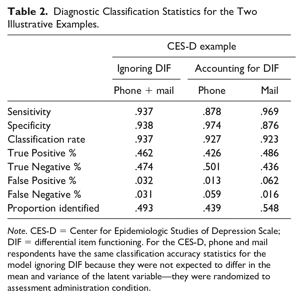
Note. CES-D = Center for Epidemiologic Studies of Depression Scale; DIF = differential item functioning. For the CES-D, phone and mail respondents have the same classification accuracy statistics for the model ignoring DIF because they were not expected to differ in the mean and variance of the latent variable—they were randomized to assessment administration condition.

Figure 3 shows how DIF on the CES-D affects sensitivity and specificity across a range of cutscores or quantiles in the latent variable score distribution. Although DIF seems to have a similar impact on sensitivity across cutscores, DIF appears to have a greater impact on specificity when the cutscore is at low levels of the construct, and appears to have little impact when the cutscore is high. As noted above, specificity is the proportion of respondents below the latent variable cutscore that are also below the cutscore on the CES-D summed score. For example, suppose that a researcher wishes to identify respondents above the 10th percentile, defined by a summed cutscore greater than or equal to 2 and a theta cutscore greater than or equal to −1.28. Chan et al. (2004) suggest that for items with DIF, thresholds in the low end of the latent variable were smaller for mail respondents than for phone respondents. As a result, when a mail and a phone respondent have the same score at the low end of the latent variable (i.e., a latent score around −1.28), the mail respondent is more likely to have a summed score higher than 2 than the phone respondent. Thus, the mail respondent might be more likely to be caught by the screener using a cutscore of 2, yielding a high false positive rate and low specificity. Similarly, higher thresholds for phone respondents (relative to the mail respondents) at the low level of the latent variable are associated with lower summed scores, a lower likelihood to be caught by the screener using the cutscore of 2, high false negatives rates and specificity, and low sensitivity.

Figure 3.

Sensitivity and specificity at different screening cutscores in the CES-D example.

Simulation Study

The previous section illustrated the proposed method via application. This section describes a simulation study that sought to answer two questions about the proposed method. First, how well does the simulation-based method recover the estimates provided by Lai et al.’s (2019) analytical method in the case of binary items (for which both methods can be used)? Second, how many iterations of the simulation are needed to obtain stable estimates of screening performance?

Simulation Specification

The population model was a standardized categorical factor model with binary items specified using the delta parameterization. Data were generated under three settings: (a) a fully invariant condition, (b) a condition in which the focal group had a higher mean (.50) and variance (1.5) than the reference group (mean of 0 and variance of 1), and (c) a condition in which there were violations of invariance in the factor loadings (e.g., the last two items for the focal group had factor loadings half of the size of the reference group) and thresholds (e.g., first two thresholds for the focal group had thresholds 0.50 higher than the reference group). There were the same number of cases in the reference and focal groups.

We varied the number of items (5 to 15) and the number of cases sampled (1,000, 5,000, 10,000, 25,000; as in Step 1 of the general procedure described above) to estimate variability of the sensitivity and specificity estimate. The scale of the items was set to unity. Factor loadings per condition were equally spaced between 0.3 and 0.7 (i.e., for a condition with seven items, factor loadings were 0.300, 0.367, 0.433, 0.500, 0.567, 0.633, and 0.700). The residual variance was 1 minus the factor loading squared for each respective item. The thresholds for all items were simulated to be zero, so each response had a 50% chance of being endorsed. In this fully crossed simulation, there were 132 conditions examined (11 number of items x 3 invariance settings x 4 numbers of cases sample), with 1,000 replications per condition.

Procedure for Simulation Study

First, the analytical approach (from the R code in Lai et al., 2019) was used to estimate sensitivity and specificity per group using the factor loadings, thresholds, and residual variances. Then, the loadings and thresholds were transformed to a and b parameters in the IRT metric using the following relations (Wirth & Edwards, 2007):

a_{j} = \frac{D λ_{j}}{\sqrt{1 - λ_{j}^{2}}}; b_{j} = \frac{τ_{j}}{λ_{j}}

(3)

In this case, D is a scaling constant of 1.7 used to convert IRT logistic estimates to normal-ogive estimates, λ is the factor loading in the factor analysis metric, and τ is the threshold in the factor analysis metric. The a- and b-parameters (in the IRT metric) were then used to estimate sensitivity and specificity using our proposed simulation approach (with R functions presented in the supplementary materials, available online). Our proposed procedure would be deemed comparable to the analytical approach from Lai et al. (2019) if it is able to recover the same estimates of sensitivity and specificity. Recovery was assessed by estimating relative bias (i.e., difference between sensitivity across the two approaches, divided by the estimate of sensitivity by the analytical approach in Lai et al., 2019; same formula for specificity), and the magnitude of the estimated standard deviation of the sensitivity and specificity estimates by the simulation approach across replications. A relative bias estimate of less than 0.05 and a standard deviation around 0.01 would suggest that the simulation approach provides unbiased and stable estimates of the impact of DIF on sensitivity and specificity of a measure with binary items.

Results

Simulation results are presented in Table 3 and Tables S1 to S4 in the supplementary materials (available online). Across conditions, relative bias for sensitivity and specificity was low. Relative bias was below 0.05 for conditions in which item parameters were invariant (Table 3) and in conditions in which the item parameters were invariant, but reference and focal groups have different means and variances (see Tables S1 and S2 in the supplementary materials, available online). Finally, relative bias was below 0.05 in conditions with at least seven items for the condition where some items have DIF, and relative bias never exceeds 0.07 in conditions with fewer than seven items (see Tables S3 and S4 in the supplementary materials, available online). As expected, the standard deviation of the sensitivity and specificity estimate decreased as more cases were sampled. Across conditions, when 1,000 cases were simulated, the standard deviation of the sensitivity and specificity estimates was as high as 0.06, but the standard deviation of the estimates was consistently around 0.01 when there were 25,000 cases simulated for the simulation-based approach.

Table 3.

Relative Bias for the Sensitivity and Specificity Estimates from the Proposed Simulation Approach compared with the Analytical Approach, and Empirical Standard Deviation of the Sensitivity and Specificity Estimates per Condition.

i	Case 1: Full Invariance
	Number of cases simulated
	Relative bias: sensitivity [specificity]				Standard deviation: sensitivity [specificity] estimate
	1,000	5,000	10,000	25,000	1,000	5,000	10,000	25,000
5	.009 [.008]	.009 [.009]	.009 [.009]	.009 [.009]	.014 [.014]	.007 [.007]	.004 [.005]	.003 [.003]
6	.006 [.012]	.005 [.011]	.006 [.013]	.005 [.012]	.012 [.018]	.005 [.008]	.003 [.006]	.002 [.004]
7	.002 [.014]	.003 [.014]	.003 [.013]	.003 [.014]	.010 [.020]	.005 [.009]	.003 [.006]	.002 [.004]
8	.003 [.011]	.001 [.014]	.001 [.013]	.001 [.014]	.009 [.023]	.004 [.010]	.003 [.007]	.002 [.005]
9	.000 [.014]	−.001 [.013]	−.001 [.013]	−.001 [.013]	.008 [.025]	.004 [.012]	.002 [.008]	.002 [.005]
10	−.001 [.013]	−.001 [.011]	−.002 [.012]	−.002 [.011]	.007 [.029]	.003 [.013]	.002 [.009]	.001 [.006]
11	−.002 [.008]	−.002 [.008]	−.002 [.008]	−.002 [.009]	.007 [.032]	.003 [.014]	.002 [.010]	.001 [.006]
12	−.002 [.008]	−.002 [.005]	−.002 [.007]	−.002 [.006]	.006 [.035]	.003 [.016]	.002 [.011]	.001 [.007]
13	−.002 [.002]	−.002 [.004]	−.002 [.003]	−.002 [.003]	.006 [.039]	.002 [.017]	.002 [.012]	.001 [.008]
14	−.002 [.000]	−.002 [.000]	−.002 [.000]	−.002 [.000]	.005 [.042]	.002 [.018]	.002 [.013]	.001 [.008]
15	−.002 [−.003]	−.002 [−.034]	−.002 [−.001]	−.002 [−.003]	.005 [.046]	.002 [.020]	.003 [.014]	.001 [.009]

Note. i = number of items. Reference and focal groups would have the same estimate of sensitivity and specificity. All items are binary and the cutscore was an observed score of 3. Relative bias is the estimate of the simulation-based procedure minus the estimate of the procedure by Lai et al. (2019), divided by the estimate by the procedure of Lai et al. (2019).

Broadly, our results suggest that the simulation-based approach recovers the estimates of sensitivity and specificity from analytical procedure by Lai et al. (2019). When the screener consists of fewer than seven items, the analytical approach is recommended because the simulation-based approach led to relative bias between 3% and 6%. When the screener has more than seven items, the analytical approach and the simulation-based approach with 25,000 iterations provide similar and stable estimates. Finally, when the screener consists of polytomous items, the simulation approach may be used because an analytical method is not yet available.

General Discussion

When researchers use screening measures in heterogeneous samples, it is important to determine if the construct is being measured in the same way across groups (e.g., males vs. females). If there are systematic differences in measurement across groups (i.e., DIF), then respondents from certain groups might be overidentified or underidentified by the screening procedure. An empirical evaluation of how the presence of DIF affects screening performance can help assessment specialists understand whether a measure with DIF is still suitable for use. This article (a) proposed a simulation-based procedure for evaluating how DIF affects screening performance, (b) illustrated the procedure using a published example, (c) conducted a simulation study to evaluate the stability of the procedure and the recovery of analytical estimates of sensitivity and specificity when DIF is found in assessments with binary items, and (d) provided R functions to implement the procedure in future applications. The article makes a novel methodological contribution by extending the Millsap and Kwok (2004) procedure to match general assessment scenarios, wherein items are binary or polytomous rather than continuous.

Standard procedures for identifying whether DIF is present typically do not provide guidance on whether DIF renders the measure too biased to use for screening. Our goal was to present assessment specialists with a tool that can be used in conjunction with standard procedures to provide an understanding of how violations of measurement invariance affect decisions based on the assessment in metrics that were intuitive to understand (e.g., changes in classification accuracy, sensitivity, and specificity). Changes in screening performance (e.g., accuracy) as a result of DIF can be thought of as effect sizes that might accompany the statistical procedures that test for DIF. Also, we illustrated how this procedure might be conducted with information found in published studies, should investigators want to address this question using information in a previous report that did not examine the impact of DIF on screening performance (such as the CES-D example in text and step-by-step example in the supplementary materials, available online). If some pieces of information are not reported (e.g., mean or variance of the latent variable), we recommend contacting the original authors to obtain the information and prevent inaccurate analyses. In our case, for illustration purposes, we made some assumptions about the pieces of information that were missing.

Limitations and Future Directions

A limitation of our procedure is that it assumes that the item response model fits the data well and that item parameters and latent variable distribution per group have been estimated precisely. Therefore, we emphasize that we made those assumptions to illustrate the proposed procedure and not to guide the appropriate use of the CES-D. As such, we encourage researchers to provide as much descriptive information as possible in their DIF studies. Second, it is important to note that this procedure will be useful when the assessor is making decisions based on the observed assessment score. Measurement bias might be less of an issue when the assessor is classifying respondents based on their latent variable scores. If partial invariance is found, item response models could accommodate DIF by linking latent variable scores from respondents across groups (Edelen & Reeve, 2007). A goal of IRT is to locate respondents along the scale of the latent variable. The location in the scale of the latent variable is the score of the respondent. As long as there are some DIF-free items across groups, the scale of the latent variable per group would be the same, which makes the latent variable scores comparable. Then, the rest of the items with group-specific parameters (e.g., items with DIF) can be used to improve the precision of the score within group. A benefit of linking is that researchers could compare latent variable scores while accommodating items with DIF. Finally, a perceived limitation of our procedure may be that we cannot provide guidelines regarding how large a difference in sensitivity or specificity should be before researchers consider dropping items or stop using the assessment. However, such guidelines depend on the specific nature of the application and it is not possible to recommend specific cutoffs (Einhorn & Hogarth, 1981).

Future directions of this research include a full evaluation of the proposed procedure using Monte Carlo simulations. As the number of items and item response options increases, it is expected that item responses might behave as if they were continuous (Rhemtulla et al., 2012). Therefore, it is expected that the simulation-based procedure proposed in this study would approximate the performance of the original procedure presented by Millsap and Kwok (2004). It would be of interest to determine the conditions under which the approximation would occur. Furthermore, the proposed procedure could also be extended to examine how dropping a biased set of items changes screening performance across groups. However, at this point the procedure becomes more complicated because dropping items would limit the range of the observed score, so other adjustments of the procedure might be needed. Also, it would be interesting to extend the proposed approach to examine the effect of DIF in assessments with mixed item-types and to situations in which screening depends on multiple scores, such as when the screener is not unidimensional. Finally, it would be interesting to continue to develop effect sizes for DIF and encourage researchers to use effect sizes to describe the impact of DIF on their assessments, as opposed to assess DIF by significance testing, which is sensitive to sample size (Kleinman & Teresi, 2016; Meade, 2010).

Conclusions

Assessment specialists desire that the individuals “caught” in a screening procedure were caught because they were high (or low) on the construct being screened for, not because of their sex, ethnicity, or other group membership. Studying DIF could be helpful to understand the magnitude of health disparities across populations of interest and guide public policy. To study disparities, it is important to have assessments that allow for valid comparisons across groups, and measurement invariance is a prerequisite to make valid comparisons (Teresi et al., 2006). With this article, we encourage researchers to incorporate this procedure into their toolbox to examine how DIF affects screening performance across priority groups and prevent the use of measures that introduce meaningful bias.

Supplemental Material

difcut_supp2_r2_sent – Supplemental material for When Does Differential Item Functioning Matter for Screening? A Method for Empirical Evaluation

Supplemental material, difcut_supp2_r2_sent for When Does Differential Item Functioning Matter for Screening? A Method for Empirical Evaluation by Oscar Gonzalez and William E. Pelham in Assessment

Supplemental Material

difimpact_supp1_r2word_sent – Supplemental material for When Does Differential Item Functioning Matter for Screening? A Method for Empirical Evaluation

Supplemental material, difimpact_supp1_r2word_sent for When Does Differential Item Functioning Matter for Screening? A Method for Empirical Evaluation by Oscar Gonzalez and William E. Pelham in Assessment

Footnotes

Author’s Note

This article is dedicated to the memory of Roger E. Millsap (1954-2014). Roger, you are deeply missed by family, colleagues, and friends.

Declaration of Conflicting Interests

The author(s) declared no potential conflicts of interest with respect to the research, authorship, and/or publication of this article.

Funding

The author(s) disclosed receipt of the following financial support for the research, authorship, and/or publication of this article: The second author was supported by a grant from the National Institute on Alcohol Abuse and Alcoholism (AA026768).

ORCID iD

Oscar Gonzalez

Supplemental Material

Supplemental material for this article is available online.

References

Azocar

Arean

Miranda

Muñoz

R. F.

(2001). Differential item functioning in a Spanish translation of the Beck Depression Inventory. Journal of Clinical Psychology, 57(3), 355-365. https://doi.org/10.1002/jclp.1017

Beck

A. T.

Ward

C. H.

Mendelson

Mock

Erbaugh

(1961). An inventory for measuring depression. Archives of General Psychiatry, 4(6), 561-571. https://doi.org/10.1001/archpsyc.1961.01710120031004

Chalmers

R. P.

Counsell

Flora

D. B.

(2016). It might not make a big DIF: Improved differential test functioning statistics that account for sampling variability. Educational and Psychological Measurement, 76(1), 114-140. https://doi.org/10.1177/0013164415584576

Chan

K. S.

Orlando

Ghosh-Dastidar

Duan

Sherbourne

C. D.

(2004). The interview mode effect on the Center for Epidemiological Studies Depression (CES-D) scale: An item response theory analysis. Medical Care, 42(3), 281-289. https://doi.org/10.1097/01.mlr.0000115632.78486.1f

Edelen

M. O.

Reeve

B. B.

(2007). Applying item response theory modeling to questionnaire development, evaluation, and refinement. Quality of Life Research, 16, Article 5. https://doi.org/10.1007/s11136-007-9198-0

Einhorn

H. J.

Hogarth

R. M.

(1981). Behavioral decision theory: Processes of judgment and choice. Annual Review of Psychology, 32, 53-88. https://doi.org/10.1146/annurev.ps.32.020181.000413

Lai

M. H.

Kwok

O. M.

Yoon

Hsiao

Y. Y.

(2017). Understanding the impact of partial factorial invariance on selection accuracy: An R script. Structural Equation Modeling: A Multidisciplinary Journal, 24(5), 783-799. https://doi.org/10.1080/10705511.2017.1318703

Lai

M. H.

Richardson

G. B.

Mak

H. W.

(2019). Quantifying the impact of partial measurement invariance in diagnostic research: An application to addiction research. Addictive Behaviors, 94, 50-56. https://doi.org/10.1016/j.addbeh.2018.11.029

Lochman

J. E.

, & The Conduct Problems Prevention Research Group. (1995). Screening of child behavior problems for prevention programs at school entry. Journal of Consulting and Clinical Psychology, 63(4), 549-559. https://doi.org/10.1037/0022-006X.63.4.549

10.

Kessler

R. C.

Berglund

Demler

Jin

Koretz

Merikangas

K. R.

Wang

P. S.

, & National Comorbidity Survey Replication. (2003). The epidemiology of major depressive disorder: Results from the National Comorbidity Survey Replication (NCS-R). Journal of the American Medical Association, 289(23), 3095-3105. https://doi.org/10.1001/jama.289.23.3095

11.

Kleinman

Teresi

J. A.

(2016). Differential item functioning magnitude and impact measures from item response theory models. Psychological Test and Assessment Modeling, 58(1), 79-98.

12.

Meade

A. W.

(2010). A taxonomy of effect size measures for the differential functioning of items and scales. Journal of Applied Psychology, 95(4), 728-743. https://doi.org/10.1037/a0018966

13.

Meredith

(1993). Measurement invariance, factor analysis and factorial invariance. Psychometrika, 58, 525-543. https://doi.org/10.1007/BF02294825

14.

Millsap

R. E.

(2011). Statistical approaches to measurement invariance. Routledge.

15.

Millsap

R. E.

(2013, October 16-19). The impact of violations of measurement invariance on selection: The discrete case [Paper presentation]. Society of Multivariate Experimental Psychology, St. Pete Beach, FA.

16.

Millsap

R. E.

Kwok

O. M.

(2004). Evaluating the impact of partial factorial invariance on selection in two populations. Psychological Methods, 9(1), 93-115. https://doi.org/10.1037/1082-989X.9.1.93

17.

Radloff

L. S.

(1977). The CES-D scale: A self-report depression scale for research in the general population. Applied Psychological Measurement, 1(3), 385-401. https://doi.org/10.1177/014662167700100306

18.

Rhemtulla

Brosseau-Liard

P. É.

Savalei

(2012). When can categorical variables be treated as continuous? A comparison of robust continuous and categorical SEM estimation methods under suboptimal conditions. Psychological Methods, 17(3), 354-373. https://doi.org/10.1037/a0029315

19.

Samejima

(1969). Estimation of latent ability using a response pattern of graded scores. Psychometrika, 34(4, Pt. 2), 1-97. https://doi.org/10.1007/BF03372160

20.

Teresi

J. A.

Ramirez

Jones

R. N.

Choi

Crane

P. K.

(2012). Modifying measures based on differential item functioning (DIF) impact analyses. Journal of Aging and Health, 24(6), 1044-1076. https://doi.org/10.1177/0898264312436877

21.

Teresi

J. A.

Stewart

A. L.

Morales

L. S.

Stahl

S. M.

(2006). Measurement in a multi-ethnic society: Overview to the special issue. Medical care, 44(11 Suppl. 3), S3-S4. https://doi.org/10.1097/01.mlr.0000245437.46695.4a

22.

Thissen

Steinberg

Wainer

(1993). Detection of differential item functioning using the parameters of item response models. In Holland

P. W.

Wainer

(Eds.), Differential item functioning (pp. 67-113). Lawrence Erlbaum.

23.

Thissen

Wainer

(2001). Test scoring. Lawrence Erlbaum.

24.

Thomas

M. L.

(2011). The value of item response theory in clinical assessment: A review. Assessment, 18(3), 291-307. https://doi.org/10.1177/1073191110374797

25.

Vilagut

Forero

C. G.

Barbaglia

Alonso

(2016). Screening for depression in the general population with the Center for Epidemiologic Studies Depression (CES-D): A systematic review with meta-analysis. PLOS ONE, 11(5), Article e0155431. https://doi.org/10.1371/journal.pone.0155431

26.

Wirth

R. J.

Edwards

M. C.

(2007). Item factor analysis: Current approaches and future directions. Psychological Methods, 12(1), 58-79. https://doi.org/10.1037/1082-989X.12.1.58

27.

Youngstrom

E. A.

(2013). A primer on receiver operating characteristic analysis and diagnostic efficiency statistics for pediatric psychology: We are ready to ROC. Journal of Pediatric Psychology, 39(2), 204-221. https://doi.org/10.1093/jpepsy/jst062

Supplementary Material

Please find the following supplemental material available below.

For Open Access articles published under a Creative Commons License, all supplemental material carries the same license as the article it is associated with.

For non-Open Access articles published, all supplemental material carries a non-exclusive license, and permission requests for re-use of supplemental material or any part of supplemental material shall be sent directly to the copyright owner as specified in the copyright notice associated with the article.

0.00 MB

0.12 MB

0.46 MB