Why Might Developers Be Reluctant to Build Conservation Subdivisions? Insights from Spatial Regression Analysis

Abstract

Despite evidence that households pay more for lots or houses in conservation subdivisions, developers are sometimes reluctant to build them. I use a spatial autoregressive model to shed light on this contradiction. The presence of nearby conservation lots reduces the value of a given conservation lot. I present two possible explanations for this result: (1) Lots located close to each other are indicative of higher density, which is frowned upon by Americans, and (2) conservation lots compete for views and rural aesthetics, and the construction of one lot decreases their availability to other lots. Results for other independent variables corroborate these explanations. Developers’ reluctance to embrace conservation subdivisions in some locations might be a result of regulations that discourage their development. More research is needed on how regulations for conservation subdivisions vary across the United States and how these affect developers’ decisions.

Keywords

spatial econometric model developers conservation lots

Introduction

Conservation developments continue to attract attention (see, for example, Hawkins 2014), and they sometimes spark controversy among researchers (Arendt 2014; Gocmen 2014). Whatever its strengths and weaknesses, the concept has become more widely known among developers and planners (Arendt 2012). Its continued presence in debates about land use, particularly in rural areas, and its potential for saving environmental amenities and preserving rural character make this type of development ripe for continued study.

Historically, these subdivisions took their cue from clustered subdivisions (Nelson and Duncan 1995), where the objective was to put aside open space, but without consideration of the aesthetic or ecological benefits of that space. Much research has found that these benefits result in a premium paid for lots or houses in conservation subdivisions (e.g., Bowman, Thompson, and Colletti 2009; Hannum et al. 2012; Mohamed 2006). However, a small body of literature has raised questions about the willingness of developers to build such subdivisions. Developers’ reluctance centers on market concerns (Carter 2009), a point that is emphasized by Kopits, McConnell, and Walls (2007) and Reichert and Liang (2007). It is this contradiction in the literature that I address in this article: If conservation lots or houses on conservation lots carry a premium, why are developers sometimes reluctant to build these developments?

I shed light on this contradiction by examining how the distance between lots could reduce the value of lots in conservation subdivisions. Using the distance between lots is an admittedly simple measure, but it is easily implementable using spatial econometric analysis, and it captures spatial tendencies to either cluster or spread out.¹ I hypothesize that the price of conservation lots will be negatively affected if they are located close to other conservation lots.

I employ a spatial autoregressive (SAR) model as my main method of analysis. I choose this method because it permits a disaggregation of the regression coefficients into the following: a direct effect, which is the effect of an independent variable on the value of a given lot; an indirect effect, which is the effect of an independent variable from surrounding lots on a given lot; and the total of the direct and indirect effects. I also present results from an ordinary least squares (OLS) regression to provide a comparison with standard regression methods. As I will discuss later, diagnostic tests for this OLS model also point to the SAR model as the preferred method of analysis, as opposed to a spatial error model (SEM), another widely used method of spatial regression analysis.

Consistent with my hypothesis, the SAR model reveals that the presence of nearby conservation lots and certain characteristics that indicate that lots are located close to each other reduce the value of a given lot. I cannot definitively explain why conservation lots located close to each other may negatively affect each other’s prices. I present two possibilities: (1) Lots located close to each other are indicative of higher density, which is frowned upon by American homebuyers and thus drives down prices, and (2) conservation developments are rooted in environmental benefits, views, and rural aesthetics, and conservation lots compete with each other for these features; the construction of one lot decreases the availability of these desirable features to others. Taken together, the results demonstrate why developers may sometimes be reluctant to build conservation subdivisions. Data for these analyses come from South Kingstown, Rhode Island, an area that has been the subject of previous analysis on the value of conservation lots.

The article proceeds as follows. The “Price Premiums for Conservation Lots but Concerns Among Developers” section provides a brief review of the pertinent literature. The “Spatial Model Specifications” section presents methodological details of the SAR model. In the “Study Area and Data” section, I discuss the study area and the data. In the “Results and Discussion” section, I present and discuss the results. The “Conclusion” section concludes.

Price Premiums for Conservation Lots but Concerns Among Developers

Conservation subdivisions are an iteration of clustered subdivisions, which have been around for a long time (Whyte 1964). However, today’s conservation subdivisions go beyond merely clustering lots to serve important ecological functions such as limiting stormwater runoff (Berke et al. 2003; Carter 2009; Lenth, Knight, and Gilgert 2006; Taylor, Brown, and Larsen 2007; Williams and Wise 2009), protecting wildlife and preserving habitats (Gonzalez-Abraham et al. 2007; Hostetler and Drake 2009), providing natural climate control (Berke et al. 2003), and limiting the need for lawn maintenance (Dramstad, Olson, and Forman 1996). Research has shown that these ecological benefits can result in higher levels of homeowner satisfaction (Kaplan, Austin, and Kaplan 2004).

To be sure, some researchers question whether conservation subdivisions achieve their intended environmental benefits (Feinberg et al. 2015; Gocmen 2014). Lenth, Knight, and Gilgert (2006) found no advantages for wildlife in a study in Colorado, and Taylor, Brown, and Larsen (2007) found only limited success in reducing the fragmentation of forests. Other research finds that developers do not pay sufficient attention to harnessing the benefits of conservation subdivisions (Beuschel and Rudel 2010; Crick and Prokopy 2009; Ryan 2006).

However, Arendt (2014) argued that the developments examined by these researchers are merely clustered subdivisions, and that the potential benefits will be achieved provided that the design of the subdivisions pays attention to ecological conservation. Indeed, the trend has been toward the preservation of land that is ecologically valuable, which amplifies the environmental benefits of conservation developments (Arendt 2004). And there is a body of evidence that homeowners pay more for these features (Bowman, Thompson, and Colletti 2009; Hannum et al. 2012; Pejchar et al. 2007). Thus, notwithstanding the occasional article that questions their environmental benefits, it is now widely accepted by scholars that conservation subdivisions—provided they meet design guidelines—produce positive environmental benefits and that households are willing to pay for these benefits and the rural character of these subdivisions (e.g, Mohamed, 2006; Mohamed, 2010).

Despite the premium for lots and houses in conservation subdivisions, developers have not wholeheartedly embraced them. Scholars have proposed many explanations for their reluctance to build conservation lots. Among these are the lack of a supportive regulatory environment (Allen et al. 2012; Bowman and Thompson 2009; Carter 2009; Gocmen 2013), community opposition (Bjelland et al. 2006), and developers’ reluctance to experiment with new designs (Carter 2009; Gyourko and Rybczynski 2000).

Hints as to why developers may be reluctant to build conservation lots come from Reichert and Liang (2007) and Kopits, McConnell, and Walls (2007). These authors highlighted the trade-off between private land space and common open space that households grapple with when buying properties in conservation subdivisions. In conservation subdivisions, households give up the former in exchange for the latter. According to Reichert and Liang (2007, p. 245), the homeowners they studied preferred “to own a two-acre parcel of land that allows for some degree of openness or separation between houses, rather than have access to a large common open space.” Kopits, McConnell, and Walls reported similar results. They found that while households valued open space in their subdivision or a vacant lot next to them, households valued their private open space even more. The authors found that households had a “small willingness” (Kopits, McConnell, and Walls 2007, p. 1196) to trade their private space for subdivision open space, but they cautioned that this result might be pertinent only when there is a large amount of surrounding open space.

The results of Reichert and Liang (2007) and Kopits, McConnell, and Walls (2007) point to the interplay between the design of conservation subdivisions on one hand, and density and aesthetics, including visibility, on the other hand. Many scholars have documented Americans’ preference for homes on large suburban lots (Ahluwalia 1999), low density (Danielsen, Lang, and Fulton 1999; Gordon and Richardson 1997; Matthews and Turnbull 2007),² and views of open space or forested land (Paterson and Boyle 2002). The clustering of lots in conservation subdivisions reflects this predicament: Conservation lots provide the environmental benefits, views, and rural aesthetic that homeowners are willing to pay for, but they do so by increasing the density of the built lots and potentially robbing some households of the very benefits they are hoping to buy into. Thus, there could be spatial competition for the desirable features of conservation lots.

Indeed, in the sample examined for this article, the average size of conservation lots is 0.48 acres, while the average size of conventional lots is 0.72 acres. I present these numbers at this point because they are consistent with the literature that conservation lots are considerably smaller than conventional lots, which leads to higher density, less views, and less rural character, thus negating the reasons why households may purchase conservation lots.

It is precisely these tensions of conservation lots that I will examine in this article: whether buyers pay more for the direct benefits of developed conservation lots but pay less when other lots are nearby.

Spatial Model Specifications

The underlying reason for presenting a spatial model is that the market for a given lot is influenced by the selling price of nearby lots. Thus, we are estimating the effect of independent variables on the price of lot i while accounting for the effect of neighboring lots. This follows from what is often referred to as the “first law of geography”: “Everything is related to everything else, but closer things more so” (attirbuted to Tobler 1979)–this is a quote widely attributed to Tobler, and I cannot find the book with it. I therefore changed to wording to say “attributed to”. Anselin and Bera (1998, p. 241) further defined the concept as follows:

Spatial autocorrelation can be loosely defined as the coincidence of value similarity with locational similarity. In other words, high or low values for a random variable tend to cluster in space (positive spatial autocorrelation) or locations tend to be surrounded by neighbors with very dissimilar values (negative spatial autocorrelation). Of the two types of spatial autocorrelation, positive autocorrelation is by far the more intuitive.

Spatial dependence is especially important when considering land values, because while each lot has unique characteristics, nearby lots—even lots in different subdivisions—tend to share characteristics. For example, they may be close to the same main road, have similar topography, and have public water and sewer. In a spatial econometric model, this “spatial autocorrelation” is captured in a spatial weights matrix.

A number of spatial econometric models are employed by various researchers. I focus on the SAR model because the coefficients produced by this model can be disaggregated into direct, indirect, and total effects, and because diagnostic tests reveal it to be a more appropriate approach when compared with other widely used spatial models.³

The SAR model proceeds on the assumption that spatial dependence is the result of omitted variables. In matrix form, it is written as

Y = ρ W Y + x β + ϵ,

where Y is an n × 1 vector of housing prices, W is an n × n spatial weights matrix, X is an n × k matrix of independent variables, $β$ is a k × 1 vector of regression coefficients, and $ρ$ is a measure of the strength of spatial dependence. As in OLS regressions, the SAR model assumes that $ϵ$ is normally distributed with 0 mean and fixed variance.

The SAR model takes explicit account of the effects of neighboring lots on the selling prices of a given lot, consistent with the intuition that the characteristics of neighboring lots are important. Thus, the selling price of lot i is a function of independent variables present on both lot i and neighboring lots j₁, j₂, j₃, and so on. In the presence of neighboring influences, the assumptions of uncorrelated error terms and independent observations are violated. Furthermore, the inverse matrix (I_n − ρW)⁻¹ in the SAR model means that spillover effects onto neighboring lots are taken into account.

Spatial weight matrices can be of different types depending on how one defines a “neighbor.” In this study, I use a row-standardized distance-based weights matrix, W, which I set at a limit of 500 feet measured from the centroid of one lot to another. I chose 500 feet as the cutoff point because this is the distance that is now widely used in spatial econometric analysis of housing prices (Conway et al. 2008; Griswold et al. n.d.; Whitaker and Fitzpatrick 2016).⁴ For computational ease, I created W in Stata using scripts provided by Jeanty (2010). This matrix was exported in Matlab-readable form, and the spatial econometric analyses were performed in Matlab. I chose Matlab to perform the analysis because it provides direct and indirect effects of each independent variable.

Study Area and Data

Data for this study come from the Town of South Kingstown, Rhode Island. Beginning in the 1990s, South Kingstown adopted open-space measures as a defining feature of its land-use policies. Among these measures was the promotion of conservation subdivisions, with the proposed designs taking their cues from Arendt (1999, 2004). Indeed, South Kingstown can be considered a good location for conservation subdivisions: It is mostly suburban and exurban, is losing forests, and is consuming land at a faster rate than population growth (Mohamed 2006). Furthermore, as the OLS results will show, the land market in South Kingstown is broadly representative of the United States.

Data were obtained from property transaction records and a Geographic Information System (GIS) maintained by the Town of South Kingstown. The transaction prices are for vacant lots in developed subdivisions. These lots were bought by builders, and the transaction prices represent value that builders would recoup from households after constructing a house on the lot.

I began the analyses with randomly selected vacant conservation, conventional, and minor lots that were sold between 1993 and 2004. These lot types were coded as dummy variables, with conventional lots serving as the reference variable. (As defined in South Kingstown, minor lots are those that are located in subdivisions that are subject to fewer improvement standards because the subdivision contains five or fewer lots. They are often built on irregularly shaped lots.) Because of the 500-foot cutoff that I used to define neighbors, I was left with 176 observations. As is typical in many models of land prices, I log the selling price and the lot size (Adams et al. 1968; Chicoine 1981; Colwell and Sirmans 1980; Guntermann 1997). This log–log formulation provides an elasticity of prices with respect to land size.

The independent variables of interest along with their summary statistics and expected signs are shown in Table 1. Because of the previously mentioned discussions on conservation lots, I expect the regression coefficient on this variable to be positive. The minor-lots variable is expected to be negative because these are lots that are built on irregularly shaped parcels and are built to fewer standards (Mohamed 2006). Because there is diminishing marginal utility to additional land, a point noted in numerous studies (Brownstone and De Vany 1991; Chicoine 1981; Colwell and Sirmans 1993), the coefficient on land size is expected to be negative. The year in which the lot was developed provides a measure of inflation; it is expected to be positive as the data cover a period of steadily increasing land prices in the study area.

Table 1.

Descriptive Statistics of Independent Variables (N = 176).

Independent Variables	M	SD	Minimum Value	Maximum Value	Expected Sign	Justification for Sign from Previous Research
Conservation lots (1 if yes, 0 if no)	0.48	0.50	0	1	+	Mohamed (2006); Bowman, Thompson, and Colletti (2009); Hannum et al. (2012)
Minor lots (1 if yes, 0 if no)	0.08	0.27	0	1	−	Mohamed (2006)
Average lot size, acres	0.62	0.51	0.22	1.64	−	Brownstone and De Vany (1991), Chicoine (1981), Colwell and Sirmans (1993)
Year in which developed lots were sold	5.20	2.02	1	8	+	Colwell and Munneke (1997)
Public water (1 if yes, 0 if no)	0.77	0.42	0	1	+	Knaap (1985), Nelson and Knaap (1987)
Public sewer (1 if yes, 0 if no)	0.40	0.49	0	1	+	Knaap (1985), Nelson and Knaap (1987)
Mean distance to scenic districts, feet	3,554	2,721	0	9,893	−	Correll, Lillydahl, and Singell (1978); Li and Brown (1980); Lindsey and Knaap (1999)
Number of lots in each subdivision	53.3	34.9	5	89	+	Hughes and Turnbull (1996), Thorsnes (2000)
Percentage of lot with difficult building conditions	6.7	20.5	0	100	−	Mohamed (2006)
Accessibility: Mean distance to Rt. 138 and U.S. 1, feet	2,999	1,886	113	6,348	−	Adams et al. (1968)
Time for lots to sell after recording, months	12.1	12.33	0.03	58.4	−	Mohamed (year 1)
Relative socioeconomic status of the lot as determined by median housing price in 1990 Census block group, US$1,000s	158	6.8	144	171	+	Bourassa, Hoesli, and Sun (2003); Brasington (1999)

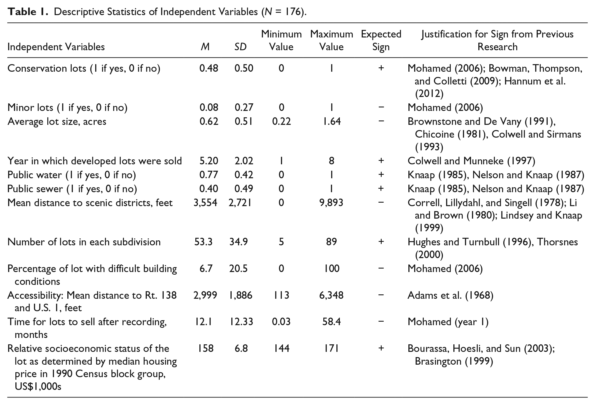
I expect the coefficients for public water and sewer to be positive as has consistently been found in other studies (Knaap 1985; Nelson and Knaap 1987). The size of the subdivision in which the lot belongs, as measured by the number of lots in the subdivision, and the relative socioeconomic status of the subdivision, as measured by median housing price of the Census block in which the lot belongs, are both expected to be positive. The former reflects developers’ ability to control neighborhood characteristics (Hughes and Turnbull 1996; Thorsnes 2000) and the latter reflects the relative socioeconomic status of the neighborhood (Bourassa, Hoesli, and Sun 2003; Brasington 1999).

The coefficient on the distance to scenic districts and the distance to the main thoroughfare, US 138, are both expected to be negative, reflecting a premium for proximity to natural areas (Adams et al. 1968; Correll, Lillydahl, and Singell 1978; Li and Brown 1980; Lindsey and Knaap 1999) and reduced travel times (Adams et al. 1968) by car in an area that depends heavily on the main thoroughfare (Mohamed 2006).

The percentage of the lot that contains difficult building conditions is a composite measure of the percent area of a lot that contains water bodies, a high water table, and steep slopes that together result in higher building costs (Mohamed 2006). Thus, the coefficient on this variable is expected to be negative. Finally, the amount of time that a lot stays on the market after it was recorded, measured in months, is expected to have a negative coefficient (Mohamed 2006).

Results and Discussion

To first test whether there is spatial collinearity, I employ Moran’s I statistic for the natural log of lot prices per acre. This statistic is 0.38 with a z-score of 4.28, which is statistically significant at the 1% level. This result confirms the initial hypothesis of spatial correlation.

Although the SAR model is of most interest in this article, I will begin by discussing the OLS results because they are the most intuitive and widely understood, and the spatial version of this model provides us with guidance on an appropriate spatial model.

Results from the OLS Model

The results for the OLS and the SAR models appear in Table 2.⁵ Conservation lots are 9% per acre more valuable than conventional lots. On the contrary, minor lots are 27% less valuable, which is not surprising because these lots are subject to lesser improvement standards, are often built on irregularly shaped lots, and are often close to busy roads.

Table 2.

Regression Results from Different Models on Price per Acre of Developed Lots.

Independent Variables	OLS Coefficients	SAR Coefficients
Conservation lots (1 if yes, 0 if no)	0.09*	0.14**
Minor lots (1 if yes, 0 if no)	−0.32**	−0.41*
Natural lot of average lot size, acres	−0.78**	−0.89*
Year in which developed lots were sold	0.08*	0.09*
Public water (1 if yes, 0 if no)	0.20*	0.27*
Public sewer (1 if yes, 0 if no)	0.12**	0.17*
Mean distance to scenic districts, feet	−4.30E−05*	−4.90E−05*
Number of lots in each subdivision	9.21E−04**	1.44E−03**
Percentage of lot with difficult building conditions	−1.03E−03**	−8.98E−04
Accessibility: Mean distance to Rt. 138 and U.S. 1, feet	2.00E−06	0.00E+00
Time for lots to sell after recording, months	5.20E−04	2.09E−04
Relative socioeconomic status of the lot as determined by median housing price in 1990 Census block group, US$1,000s	1.71E−03	1.31E−03
Adjusted r²	.78
ρ		−.236

Note. OLS = ordinary least squares; SAR = spatial autoregressive.

Significant at the 1% level. **Significant at the 5% level. ***Significant at the 10% level.

The coefficient for lot size confirms, as discovered in numerous other studies (e.g., Brownstone and De Vany 1991), that there is diminishing value to increasing lot size. Other results are also consistent with the existing literature. The value of developed lots increases at a rate of 8% per year (significant at the 1% level). Public water adds 22% per acre (significant at the 1% level) to the value of lots, and public sewer adds 13% per acre (significant at the 5% level). Builders pay about 4% more per acre of lot for every 1,000 feet the lot is located closer to a state-designated scenic district (significant at the 1% level).

Other variables that are significant at the 5% level and of small magnitude include the number of lots in a subdivision and the percentage of the lot with difficult building conditions. Each additional lot in a subdivision increases the per acre price of lots by about 0.1%, which is consistent with other research that has found that larger subdivisions carry a premium because developers are better able to control neighborhood characteristics (Hughes and Turnbull 1996; Thorsnes 2000). Each 1% increase in the area of a lot with difficult building conditions decreases the per acre value of lots by about 0.1%, which is not surprising because these lots are more expensive to build on.

Access as measured by distance to the major road in the township, US 138, is not statistically significant, most likely because the web of roads in the study area makes the specific location of a particular lot in relation to US 138 unimportant. The time for lots to sell after being recorded is not statistically significant, which is probably because of randomness in the land market during short periods of time as builders buy lots and build houses to meet short-term changes in demand. I cannot explain why the socioeconomic status of the Census-defined block group in which the lot is located is not statistically significant.

The results from the OLS regressions show that the land market in South Kingstown, Rhode Island, is broadly representative of markets across the country: There is diminishing marginal utility to additional land (Brownstone and De Vany 1991; Chicoine 1981; Colwell and Sirmans 1993; Guntermann 1997), public infrastructure such as sewer and water carries a premium as observed by many scholars (see, for example, Knaap 1985; Nelson and Knaap 1987), lots built to fewer standards sell for less (Mohamed 2006; minor lots in the parlance of regulations in South Kingstown, Rhode Island), there is a premium for access to major roads (see, for example, Adams et al. 1968) and scenic areas (see, for example, Correll, Lillydahl, and Singell 1978; Li and Brown 1980; Lindsey and Knaap 1999), and properties in larger subdivisions sell for more (Hughes and Turnbull 1996; Thorsnes 2000; operationalized in this study by the number of lots in the subdivision).

Diagnostic tests of OLS models can also provide guidance on whether to use a SAR model or SEM. This test revealed a higher Lagrange multiplier for the SAR model versus the SEM model (111.13 vs. 41.37, respectively). The test also revealed a higher robust Lagrange multiplier for the SAR model versus the SEM model (73.66 vs. 41.38, respectively). These tests reveal that the SAR model is the preferred method of spatial regression analysis.

Results from the SAR Model

The signs of the coefficients obtained in the SAR model are the same as in the OLS results above. (It is not possible to compare the coefficients directly because the coefficients for the SAR model do not represent marginal effects.) All coefficients are again found in Table 2. The SAR model also provides a better overall fit with the data, as evidenced by the log likelihood ratio of −105.7, the highest of all the models examined. The model converged within 5,000 iterations.

In the SAR model, as expected, the coefficient for lots in conservation subdivisions is positive and significant at the 5% level. Lots in minor subdivisions have less value, a result that is statistically significant at the 1% level.

The sign and statistical significance of other variables are also as expected. Among those that are significant at the 1% level are the natural log of lot size (with the expected negative sign); inflation, public water, and public sewer (all three with the expected positive sign); and distance from scenic districts (with the expected negative sign). Finally, the existence of more lots in the subdivision increases the value of lots, a result that is significant at the 5% level.

Unlike in the OLS model, the percentage of the lot with difficult building conditions is not statistically significant. As in the OLS model, accessibility, the time to sell after recording, and relative socioeconomic status are not statistically significant.

The direct, indirect, and total marginal effects produce interesting results. These effects are presented in Table 3 in the order in which I discuss them here. (I discuss only those results that are statistically significant.) The results show that the direct value of a conservation lot is about 15% per acre higher than that of a conventional lot (significant at the 5% level), but that conservation lots within 500 feet subtract from the value of a given conservation lot, reducing it by 3% per acre (significant at the 10% level). The total marginal value added to a conservation lot is 12% per acre (significant at the 5% level). The result for the indirect effect provides evidence—though of a relatively small magnitude and weak significance—that the value of conservation lots can be adversely affected by the nearby presence of other conservation lots.

Table 3.

Direct, Indirect, and Total Coefficients of the SAR Model.

Independent Variables	Total Effect	Direct Effect	Indirect Effect
Main variable
Conservation subdivisions (1 if yes, 0 if no)	0.11**	0.14**	−0.03***
Results for variables that are also indicative of higher density
Public water (1 if yes, 0 if no)	0.22*	0.28*	−0.05**
Public sewer (1 if yes, 0 if no)	0.14*	0.17*	−0.03**
Natural log of average lot size, acres	−0.72*	−0.90*	0.18*
Year in which developed lots were sold	0.08*	0.10*	−0.02*
Number of lots in each subdivision	1.17E−03*	1.46E−03**	−2.94E−04***
Results for other variables
Minor lots (1 if yes, 0 if no)	−0.33*	−0.41*	0.08**
Mean distance to scenic districts, feet	−4.00E−05*	−4.90E−05*	1.00E−05**
Percentage of lot with difficult building conditions	−7.39E−04	−9.11E−04	1.72E−04
Accessibility: Mean distance to Rt. 138 and U.S. 1, feet	0.00E+00	0.00E+00	0.00E+00**
Time for lots to sell after recording, months	1.66E−04	1.90E−04	−2.40E−05
Relative socioeconomic status of the lot as determined by median housing price in 1990 Census block group, US$1,000s	1.07E−03	1.32E−03	−2.43E−04

Note. Arranged to mirror discussions of the spatial lag effects of the SAR model. SAR = spatial autoregressive.

Significant at the 1% level. **Significant at the 5% level. ***Significant at the 10% level.

Results are also indicative of a preference for lower density and/or competition for views and rural aesthetics. A measure of clustering or dispersion in the spatial regressive model is ρ. A positive ρ is usually observed in social science data, reflecting the tendency of economic agents to cluster. The results, however, produce a negative ρ of −.236, significant at better than the 1% level. This result is not commonly found in social science data, and I interpret it to suggest a preference for lower density and/or competition for views and rural aesthetics among buyers.

Among the variables that are indicative of the preference for lower density and the value of views and rural aesthetics are public water and public sewer. Both of these variables add direct value to a lot (33% and 19%, respectively; both significant at the 1% level), and the total values are also positive (25% and 15%, respectively; both significant at the 1% level). However, the indirect effects for public water and public sewer are negative (5% and 3%, respectively; both significant at the 5% level). This means that being located within 500 feet of lots that contain public water and public sewer reduces the value of a given lot.

The result for average lot size is noteworthy. As expected, the direct and total effects are negative. As in other research (Chicoine 1981; Colwell and Munneke 1997; Colwell and Sirmans 1993), this is consistent with the diminishing marginal utility of additional land. The effects are large, which suggests that the value of lots falls rapidly as they increase in size. However, an opposite—though smaller—effect is felt from the presence of nearby lots; larger nearby lots increase the value of a given lot by about 18% per acre (significant at the 1% level). The implication is that homeowners prefer their neighbors to have larger lots.

The result for the year in which the lot was sold (a measure of inflation) also suggests an interpretation that is consistent with a preference for lower densities and/or competition for views and rural aesthetics. As expected, the direct and total effects are positive (10% and 8%, respectively; significant at the 1% level). The direct effect means that each subsequent year that a lot is sold adds 10% per acre to the value of the lot. However, the indirect effect is negative 2%, a result that is also significant at the 1% level. This result suggests that for a given lot, each subsequent year in which a nearby lot was sold reduced the value of the lot in question by 2% per acre. This suggests some anticipation in the housing market; expectations of nearby development in the future reduce the value of a current lot sale.

Although the magnitude of the results for the number of lots in each subdivision is small, they also suggest a similar interpretation. The positive direct effect (significant at the 5% level) demonstrates the premium of being located in a larger subdivision. However, the negative indirect effect suggests that being within 500 feet of a lot that is in a large subdivision reduces the value of a given lot. Although this negative indirect effect is small and significant at the 10% level, it underscores the fact that land values are lower when the land is located close to other development.

Results for Other Variables

As expected, minor lots sell for less than conventional lots. This fact is reflected in the total and direct effects, which are both significant at the 1% level. However, I cannot explain the positive indirect effect of this variable. Finally, the direct and total effects show that the farther away a lot is from a scenic district, the more its value falls. While the negative direct and total effects for this variable are expected, I cannot explain the positive indirect effect.

Conclusion

The results confirm the appeal of conservation lots: Americans are willing to pay more for them. As the SAR model results show, lots in conservation subdivisions carry a total premium of 11%. The premium that comes directly from the lot itself is 14%.

The SAR model permits us to examine the effects of nearby lots on the value of a given lot. While the indirect effect for the variable conservation lot is significant only at the 10% level, other variables provide corroborative evidence for the negative effects of properties being located close to each other. In particular,

when nearby lots have public water and sewer, the value of a given lot decreases;

when nearby lots are larger, the value of a given lot increases;

when there are expectations that nearby lots will sell, the value of a given lot decreases; and

when nearby lots are in larger subdivisions, the value of a given lot decreases.

I interpret these indirect effects to suggest that Americans prefer lower density development and that there is competition for views and rural aesthetics. The former effect is consistent with other research (Danielsen, Lang, and Fulton 1999; Gordon and Richardson 1997; Matthews and Turnbull 2007). The latter effects likely result because when views and rural aesthetics are consumed by one conservation lot, there is less available for consumption by others, which encourages property owners to seek distance away from existing or anticipated development. Of course, low-density development and views and rural aesthetics are not mutually exclusive, and both effects are likely intertwined.

The trade-off between the positive direct effects of conservation lots and the negative effects of density and competition for views and rural aesthetics gets to the larger challenges facing conservation subdivisions. How do planners fashion regulations for conservation lots such that they are financially attractive to developers? Given the results of this article and the popularity of conservation lots in the study area (see Mohamed 2006), it appears that planners there have figured out an approach in which the direct effects outweigh the indirect effects. I hypothesize that developers’ reluctance to embrace conservation subdivisions in some locations (see, for example, Allen et al. 2012; Bjelland et al. 2006; Bowman and Thompson 2009; Carter 2009; Gocmen 2013) might be a result of regulations that discourage their development rather than a lack of market demand by households. I cannot say what these inhibiting regulations might be, but some possibilities present themselves. Some jurisdictions may

not permit the layout of lots such that most or all of the lots in a subdivision have views of and easy access to common open space;

require conservation lots to be too small when compared with conventional lots;

not permit lot bonuses (an increase in the number of lots permitted if a developer builds a conservation subdivision); and

require building roads to the high standards typically found in conventional subdivisions, thus abrogating the rural aesthetic of the subdivision.

I leave a study of how regulations for conservation subdivisions vary across the United States and how these variations may affect developers’ willingness to build them for subsequent research.

Footnotes

Declaration of Conflicting Interests

The author(s) declared no potential conflicts of interest with respect to the research, authorship, and/or publication of this article.

Funding

The author(s) received no financial support for the research, authorship, and/or publication of this article.

Notes

Author Biographies

Rayman Mohamed, PhD, is an associate professor in the Department of Urban Studies and Planning, Wayne State University.

References

Adams

F. Gerard

Milgram

Grace

Green

Edward W.

Mansfield

Christine

. 1968. “Undeveloped Land Prices During Urbanization: A Micro-Empirical Study over Time.” The Review of Economics of Statistics 50:248–58.

Ahluwalia

Gopal

. 1999. “Public Attitudes Toward Growth.” Housing Economics 47 (5): 7–13.

Allen

Stephen C.

Moorman

Christopher E.

Peterson

M. Nils

Hess

George R.

Moore

Susan E.

2012. “Overcoming Socio-economic Barriers to Conservation Subdivisions: A Case-Study of Four Successful Communities.” Landscape and Urban Planning 106 (3): 244–52.

Anselin

Luc

Bera

Anil

. 1998. “Spatial Dependence in Linear Regression Models with an Introduction to Spatial Econometrics.” In Handbook of Applied Economic Statistics, edited by Ullah

Aman

Giles

David

, 237–89. New York: Marcel Dekker.

Arendt

Randall G.

1999. Growing Greener: Putting Conservation into Local Plans and Ordinances. Washington, DC: Island Press.

Arendt

Randall G.

2004. Crossroads, Hamlet, Village, Town: Design Characteristics of Traditional Neighborhoods, Old and New. Rev. ed. Chicago: APA Planning Advisory Service.

Arendt

Randall G.

2012. Conservation Design for Subdivisions: A Practical Guide to Creating Open Space Networks. Washington, DC: Island Press.

Arendt

Randall G.

2014. “Clarifying the Conservation Subdivision Design Approach.” Planetizen. Accessed May 3, 2017. http://www.planetizen.com/node/67619.

Berke

Philip

MacDonald

Joe

White

Nancy

Holmes

Michael

Line

Dan

Oury

Kat

Ryznar

Rhonda

. 2003. “Greening Development to Protect Watersheds: Does New Urbanism Make a Difference?” Journal of the American Planning Association 69 (4): 397–413.

10.

Beuschel

Vanessa

Rudel

Thomas

. 2010. “Can Real-Estate Developers Be “Green”? Sprawl, Environmental Rhetoric, and Land Use Planning in a New Jersey Community.” Society & Natural Resources 23 (2): 97–110.

11.

Bjelland

Mark D.

Maley

Michelle

Cowger

Lane

Barajas

LisaBeth

. 2006. “The Quest for Authentic Place: The Production of Suburban Alternatives in Minnesota’s St. Croix Valley.” Urban Geography 27 (3): 253–70.

12.

Bourassa

Steven C.

Hoesli

Martin

Sun

Jian

. 2003. “What’s in a View?” FAME Research Paper No. 79. https://papers.ssrn.com/sol3/papers.cfm?abstract_id=410729

13.

Bowman

Troy

Thompson

Jan

. 2009. “Barriers to Implementation of Low-Impact and Conservation Subdivision Design: Developer Perceptions and Resident Demand.” Landscape and Urban Planning 92 (2): 96–105.

14.

Bowman

Troy

Thompson

Jan

Colletti

Joe

. 2009. “Valuation of Open Space and Conservation Features in Residential Subdivisions.” Journal of Environmental Management 90 (1): 321–30.

15.

Brasington

David

. 1999. “Which Measures of School Quality Does the Housing Market Value?” Journal of Real Estate Research 18 (3): 395–413.

16.

Brownstone

David

De Vany

Arthur

. 1991. “Zoning, Returns to Scale, and the Value of Undeveloped Land.” The Review of Economics and Statistics 73:699–704.

17.

Carter

Timothy

. 2009. “Developing Conservation Subdivisions: Ecological Constraints, Regulatory Barriers, and Market Incentives.” Landscape and Urban Planning 92 (2): 117–24.

18.

Chicoine

David L.

1981. “Farmland Values at the Urban Fringe: An Analysis of Sale Prices.” Land Economics 57:353–62.

19.

Colwell

Peter F.

Munneke

Henry J.

1997. “The Structure of Urban Land Prices.” Journal of Urban Economics 41 (3): 321–36.

20.

Colwell

Peter F.

Sirmans

Clemon F.

1980. “Nonlinear Urban Land Prices.” Urban Geography 1 (2): 141–52.

21.

Colwell

Peter F.

Sirmans

Clemon F.

1993. “A Comment on Zoning, Returns to Scale, and the Value of Undeveloped Land.” The Review of Economics and Statistics 75:783–86.

22.

Conway

Delores

Christina Q.

Wolch

Jennifer

Kahle

Christopher

Jerrett

Michael

. 2008. “A Spatial Autocorrelation Approach for Examining the Effects of Urban Greenspace on Residential Property Values.” The Journal of Real Estate Finance and Economics 41 (2): 150–69.

23.

Correll

Mark R.

Lillydahl

Jane H.

Singell

Larry D.

1978. “The Effects of Greenbelts on Residential Property Values: Some Findings on the Political Economy of Open Space.” Land Economics 54:207–17.

24.

Crick

Julie

Prokopy

Linda S.

2009. “Prevalence of Conservation Design in an Agriculture-Dominated Landscape: The Case of Northern Indiana.” Environmental Management 43 (6): 1048–60.

25.

Danielsen

Karen A.

Lang

Robert E.

Fulton

William

. 1999. “Retracting Suburbia: Smart Growth and the Future of Housing.” Housing Policy Debate 10 (3): 513–40.

26.

Dramstad

Wenche E.

Olson

James D.

Forman

Richard T. T.

1996. Landscape Ecology Principles in Landscape Architecture and Land-Use Planning. Washington, DC: Island Press.

27.

Feinberg

Daniel S.

Hostetler

Mark E.

Reed

Sarah E.

Pienaar

Elizabeth F.

Pejchar

Liba

. 2015. “Evaluating Management Strategies to Enhance Biodiversity in Conservation Developments: Perspectives from Developers in Colorado, USA.” Landscape and Urban Planning 136:87–96.

28.

Gocmen

Asligul

. 2013. “Barriers to Successful Implementation of Conservation Subdivision Design: A Closer Look at Land Use Regulations and Subdivision Permitting Process.” Landscape and Urban Planning 110:123–33.

29.

Gocmen

Asligul

. 2014. “Assessing the Environmental Merits of Conservation Subdivision Design.” Journal of Planning Education and Research 34 (2): 203–20.

30.

Gonzalez-Abraham

Charlotte E.

Radeloff

Volker C.

Hammer

Roger B.

Hawbaker

Todd J.

Stewart

Susan I.

Clayton

Murray K.

2007. “Building Patterns and Landscape Fragmentation in Northern Wisconsin, USA.” Landscape Ecology 22 (2): 217–30.

31.

Gordon

Peter

Richardson

Harry W.

1997. “Are Compact Cities a Desirable Planning Goal?” Journal of the American Planning Association 63 (1): 95–106.

32.

Griswold

Nigel G.

Calnin

Benjamin

Schramm

Michael

Anselin

Luc

Boehnlein

Paul

. n.d. “Estimating the Effect of Demolishing Distressed Structures in Cleveland, OH, 2009-2013: Impacts on Real Estate Equity and Mortgage-Foreclosure.” Western Reserve Land Conservancy Thriving Communities Institute, Cleveland, IL.

33.

Guntermann

Karl L.

1997. “Residential Land Prices Prior to Development.” Journal of Real Estate Research 14 (1): 1–17.

34.

Gyourko

Joseph

Rybczynski

Witold

. 2000. “Financing New Urbanism Projects: Obstacles and Solutions.” Housing Policy Debate 11 (3): 733–50.

35.

Halvorsen

Robert

Palmquist

Raymond

. 1980. “The Interpretation of Dummy Variables in Semilogarithmic Equations.” The American Economic Review 70 (3): 474–75.

36.

Hannum

Christopher

Laposa

Steven

Reed

Sarah

Pejchar

Liba

Lindsay

. 2012. “Comparative Analysis of Housing in Conservation Developments: Colorado Case Studies.” Journal of Sustainable Real Estate 4 (1): 149–76.

37.

Hawkins

Christopher V.

2014. “Landscape Conservation Through Residential Subdivision Bylaws: Explanations for Local Adoption.” Landscape and Urban Planning 121:141–48.

38.

Hostetler

Mark E.

Drake

David

. 2009. “Conservation Subdivisions: A Wildlife Perspective.” Landscape and Urban Planning 90 (3–4): 95–101.

39.

Hughes

William T.

Turnbull

Geoffrey K.

1996. “Uncertain Neighborhood Effects and Restrictive Covenants.” Journal of Urban Economics 39 (2): 160–72.

40.

Jeanty

Wilner

. 2010. “SPWMATRIX: Stata Module to Generate, Import, and Export Spatial Weights.” Accessed May 3, 2017. http://ideas.repec.org/c/boc/bocode/s457111.html.

41.

Kaplan

Rachel

Austin

Maureen E.

Kaplan

Stephen

. 2004. “Open Space Communities: Resident Perceptions, Nature Benefits, and Problems with Terminology.” Journal of the American Planning Association 70 (3): 300–12.

42.

Knaap

Gerrit J.

1985. “The Price Effects of Urban Growth Boundaries in Metropolitan Portland, Oregon.” Land Economics 61:26–35.

43.

Kopits

Elizabeth

McConnell

Virginia

Walls

Margaret

. 2007. “The Trade-Off Between Private Lots and Public Open Space in Subdivisions at the Urban-Rural Fringe.” American Journal of Agricultural Economics 89 (5): 1191–97.

44.

Lenth

Buffy A.

Knight

Richard L.

Gilgert

Wendell C.

2006. “Conservation Value of Clustered Housing Developments.” Conservation Biology 20 (5): 1445–56.

45.

Levine

Jonathan

Frank

Lawrence D.

2007. “Transportation and Land-Use Preferences and Residents’ Neighborhood Choices: The Sufficiency of Compact Development in the Atlanta Region.” Transportation 34 (2): 255–74.

46.

Lewis

Paul G.

Baldassare

Mark

. 2010. “The Complexity of Public Attitudes Toward Compact Development.” Journal of the American Planning Association 76 (2): 219–37.

47.

Mingche M.

Brown

H. James

. 1980. “Micro-Neighborhood Externalities and Hedonic Housing Prices.” Land Economics 56:125–41.

48.

Lindsey

Greg

Knaap

Gerrit

. 1999. “Willingness to Pay for Urban Greenway Projects.” Journal of the American Planning Association 65 (3): 297–313.

49.

Matthews

John W.

Turnbull

Geoffrey K.

2007. “Neighborhood Street Layout and Property Value: The Interaction of Accessibility and Land Use Mix.” The Journal of Real Estate Finance and Economics 35 (2): 111–41.

50.

Mohamed

Rayman

. 2006. “The Economics of Conservation Subdivisions: Price Premiums, Improvement Costs, and Absorption.” Urban Affairs Review 41 (3): 376–99.

51.

Mohamed

Rayman

. 2010. “Are Profits from Subdivision Development Higher in Areas With More Regulations? A Case Study of South Kingstown, Rhode Island and Some Implications for Land Use Planning.” Housing Policy Debate, 20 (3): 429-456.

52.

Mohamed

Rayman

vom Hofe

Rainer

Mazumder

Sangida

. 2014. “Jurisdictional Spillover Effects of Sprawl on Injuries and Fatalities.” Accident Analysis & Prevention 72 (1): 9–16.

53.

Nelson

Arthur C.

Duncan

James B.

1995. Growth Management Principles and Practices. Chicago: Planners Press, American Planning Association.

54.

Nelson

Arthur C.

Knaap

Gerrit J.

1987. “A Theoretical and Empirical Argument for Centralized Regional Sewer Planning.” Journal of the American Planning Association 53 (4): 479–86.

55.

Paterson

Robert W.

Boyle

Kevin J.

2002. “Out of Sight, Out of Mind? Using GIS to Incorporate Visibility in Hedonic Property Value Models.” Land Economics 78 (3): 417–25.

56.

Pejchar

Liba

Morgan

Peter M.

Caldwell

Margaret R.

Palmer

Carl

Daily

Gretchen C.

2007. “Evaluating the Potential for Conservation Development: Biophysical, Economic, and Institutional Perspectives.” Conservation Biology 21 (1): 69–78.

57.

Reichert

Alan K.

Liang

Hsin-Yu

. 2007. “An Economic Analysis of Real Estate Conservation Subdivision Developments.” Appraisal Journal 75 (3): 236–45.

58.

Ryan

Robert L.

2006. “Comparing the Attitudes of Local Residents, Planners, and Developers About Preserving Rural Character in New England.” Landscape and Urban Planning 75 (1–2): 5–22.

59.

Taylor

Jason J.

Brown

Daniel G.

Larsen

Larissa

. 2007. “Preserving Natural Features: A GIS-Based Evaluation of a Local Open-Space Ordinance.” Landscape and Urban Planning 82 (1–2): 1–16.

60.

Thorsnes

Paul

. 2000. “Internalizing Neighborhood Externalities: The Effect of Subdivision Size and Zoning on Residential Lot Prices.” Journal of Urban Economics 48 (3): 397–418.

61.

Tobler

Waldo

. 1979. “Cellular Geography.” In Philosophy in Geography, edited by Gale

Stephen

Olssohn

Gunnar

, 379–86. Dordrecht: Reidel.

62.

Whitaker

Stephan

Fitzpatrick

Thomas J.

2016. “Land Bank 2.0: An Empirical Evaluation.” Journal of Regional Science 56 (1): 156–75.

63.

Whyte

William H.

1964. Cluster Development. 1st ed. New York: American Conservation Association.

64.

Williams

Evan S.

Wise

William R.

2009. “Economic Impacts of Alternative Approaches to Storm-Water Management and Land Development.” Journal of Water Resources Planning and Management 135 (6): 537–46.