



Abstract
We highlight the use of a newer method—emerging hot spot analysis of space-time cubes from defined locations—for examining the spread of housing vacancy in large Ohio MSAs. Using this method, we discovered that many Ohio MSAs concurrently experienced spread, contraction, and vacancy stabilization in census tracts located adjacent to, or within close proximity of, one another. These results indicate that vacancy proliferation is not solely a matter of geographic determinism, whereby high vacancy in one tract predicts high vacancy in neighboring tracts in future years. We also found that vacancy spread at the tract level is associated with population dynamics at the neighborhood, city, and MSA levels. Our findings suggest that vacancy reduction initiatives should account for population trends at various geographic scales, not just physical conditions within a particular neighborhood or tract.
Introduction
Sophisticated methods for studying changes in the physical forms of cities that are losing population (i.e. “shrinking cities”) are lacking in the literature. In their review of spatial metrics, Reis, Silva and Pinho (2016) found 123 methods for studying urban growth, but only 15 for studying shrinkage. In this research note, we highlight the use of a newer method—emerging hot spot analysis of space-time cubes from defined locations—to examine the spread of housing vacancy, a common indicator of shrinkage (Reis, Silva and Pinho 2016; Couch and Cocks 2013). The method has existed in ESRI's ArcGIS Pro since 2017 (Bennett, D; costa and Vale 2017), but has not been previously applied to the study of vacancy. 1 This method differs from traditional hot spot methodologies in that it identifies statistically significant spatiotemporal relationships (i.e. spatial change over time).
We begin with a description of why vacancy is a salient issue and how researchers have studied its spatial patterns. We then describe the aforementioned method in detail, and investigate how the spread of vacancy relates to population change—another indicator of shrinkage—at various geographic scales. Then, we present the results of our analyses, as well as the urban planning and policy implications of our methodology and findings.
Why Vacancy Matters: Vacant properties reduce property values and tax revenues (Whitaker and Fitzpatrick IV 2013), increase a community's service costs and need for demolitions (Morckel 2017; Schilling 2009), and discourage private investment (Mallach 2012). Moreover, there is increasing evidence that vacant properties adversely affect the health of the people who live near them due to conditions like trash build up, overgrown vegetation, vermin, and background lead exposure (Castro et al. 2019; Garvin et al. 2013; Teixeira and Wallace 2013). In line with Wilson and Kelling’s (1982) “broken windows” hypothesis, vacancies correlate with elevated property and violent crime rates (Roth 2019; Boessen and Chamberlain 2017; Cui and Walsh 2015; Spelman 1993), and contribute to residents’ poor mental health by reducing “cues to care” and increasing social disorder at the neighborhood-level (Wang and Immergluck 2018; Cagney et al. 2014; Nassauer and Raskin 2014). Because vacancies tend to cluster in the most distressed neighborhoods (Morckel 2014b), they have a disproportionate impact on vulnerable populations like minorities, the poor, and recipients of rental vouchers (Silverman, Yin and Patterson 2013), making the problem of property vacancy a social and environmental justice concern (Lord 1995). For these reasons, it is important for urban planners and policy makers to understand how vacancy proliferates.
Prior Research on Housing Vacancy: Many studies demonstrate that levels of vacancy vary from neighborhood to neighborhood and/or city to city. The majority of these studies explore changes in vacancy rates within fixed political boundaries (without consideration for neighboring units), or they predict vacancy levels in different places (e.g. neighborhoods) at one point in time, using cross-sectional measures [e.g. Immergluck (2016) for census tracts in 50 metropolitan areas; Morckel (2014a) for block groups in Columbus, OH; Silverman, Yin and Patterson (2013) for census tracts in Buffalo, NY; Wilson, Margulis and Ketchum (1994) for census tracts in Cleveland, OH].
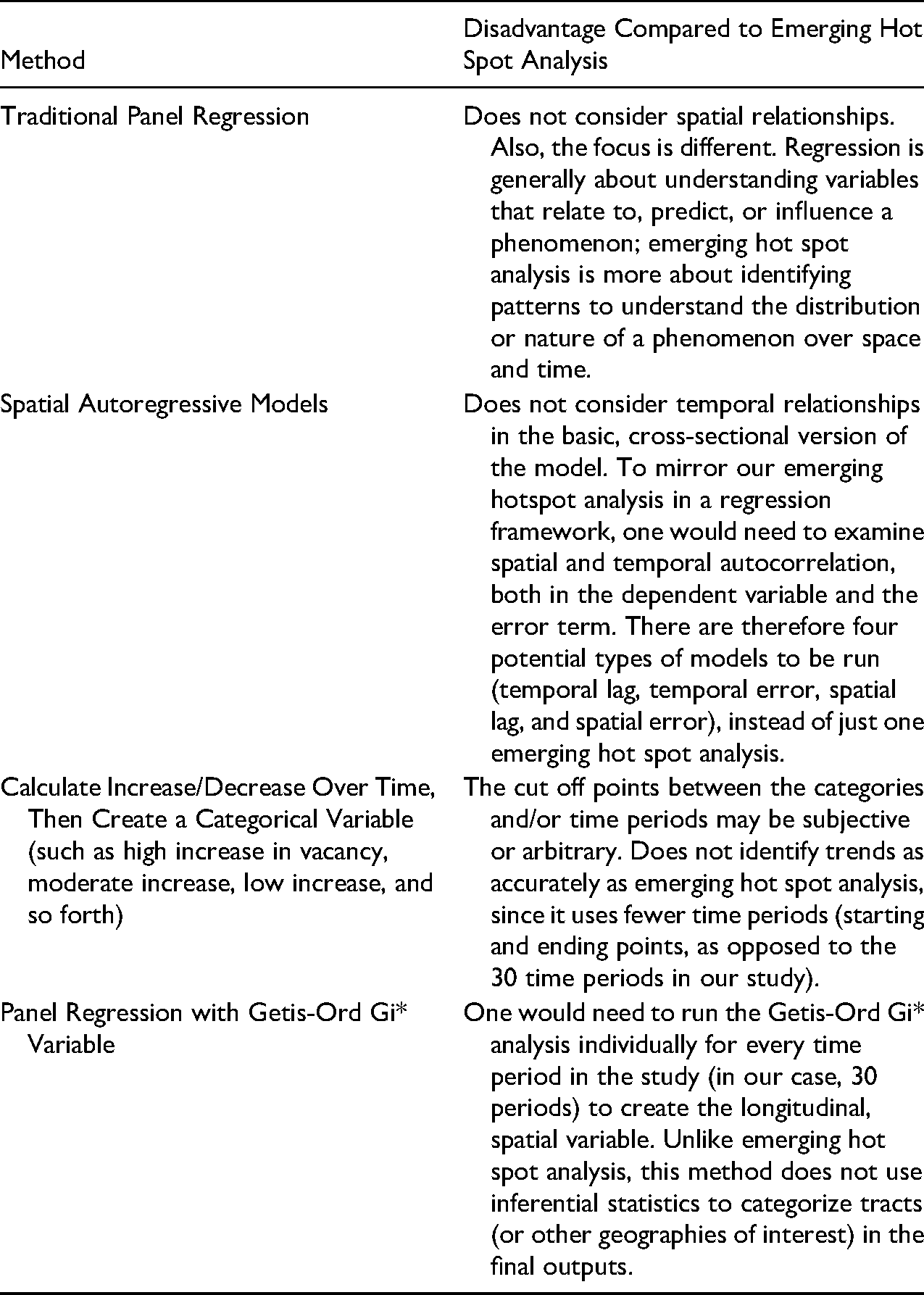
Prior studies of changes in vacancy have several limitations. First, they usually do not consider whether changes or differences in vacancy rates represent real statistically significant changes. Second, they do not examine whether vacancy within a geographic unit of interest (e.g. a neighborhood or tract) is statistically significantly different relative to other units in the sampling frame (e.g. the other neighborhoods or tracts). Third, they do not use spatial statistics and thus cannot clearly identify if or how vacancy is concentrating or spreading. Fourth, to the extent that these studies examine the spatial clustering of vacancies, they do not examine changes in these patterns of clustering over time. Vacancy may increase in a small geographic area like a census block group or tract for example, but this does not necessarily mean it is moving outward into adjacent geographic units. The methodology we present herein addresses these limitations. Moreover, Table 1 provides a brief summary of other methods that could be used to examine spatial and/or temporal changes in vacancy, and why our method is preferable.
Other Common Methods to Examine Spatial and/or Temporal Change.
Population Change & Regional Context: Because many studies have shown an association between property vacancy and population change, we also consider the effects of local and regional population dynamics on vacancy spread. Ribant and Chen (2020) found that shrinking cities have higher levels of vacant housing than growing cities, and the extent of vacancy depends on regional context. Of the 367 U.S. shrinking cities they identified, 60.5 percent were large central cities (N = 81) or shrinking suburbs of those central cities (N = 141). Earlier work by Morckel (2013) also supports the importance of regional population dynamics when measuring or predicting vacancy. She found that the odds of a house being abandoned in Youngstown, Ohio—a shrinking city located in a shrinking MSA—were significantly greater than the odds of a similar house in a similar neighborhood being abandoned in Columbus, Ohio—a growing city located in a growing MSA. However, neither of these works [Ribant and Chen (2020) nor Morckel (2013)] were longitudinal—and thus, they do not identify how the spread of vacancy varies at different scales. The new method outlined herein allows for such an examination.
The potential importance of geographic scale is further emphasized by Segers et al. (2020) who argue that more diverse meanings for shrinkage are found by connecting shrinkage on the local level to growth on larger planning and policy levels—a concept they call “shrinkage in growth” (p. 8). If we find that spatial patterns of vacancy differ by place and/or scale, it would emphasize how vacancy reduction initiatives (which are usually implemented at the neighborhood-level) might be more effective if paired with interventions that account for the broader context of population change.
Methods
Sampling Frame: Using emerging hot spot analysis, we examine census tract-level vacancy spread and population change for all Ohio MSAs with at least 500,000 residents. These MSAs (listed alphabetically by central city) are Akron, Cincinnati, Cleveland, Columbus, Dayton, Toledo, and Youngstown. Limiting the study to only Ohio MSAs controls for differences in vacancy rates that might otherwise be attributable to differences in state policy environments, such as the ability to land bank or to have vacant property registration ordinances (Lee, Terranova and Immergluck 2013). These MSAs are also a suitable sampling frame because of variation in their population trends and economic trajectories of their sub-metropolitan entities (e.g., central cities, suburbs, exurbs), despite being located in the same state.
Space-Time Cubes: The creation of a space-time cube is a prerequisite for running an emerging hot spot analysis. Space-time cubes are descriptive statistics comprised of “bins,” with each bin having a value (in our case, a vacancy rate) with ‘X’ and ‘Y’ dimensions indicating location, and ‘Z’ (vertical space) representing time. 2 To reduce edge effects, we created a space-time cube for the entire state of Ohio before running the emerging hot spot analysis in ArcGIS Pro and examining the results by MSA. 3 We defined MSA boundaries using the U.S. Census Bureau's 2018 delineations of Core Based Statistical Areas (Manson et al. 2019), and obtained quarterly, census tract level vacancy data from the United States Postal Service (USPS). We calculated vacancy rates by summing the number of vacant and no-stat (non-functional) residential units in the USPS dataset 4 , then dividing by the total number of units per tract. We used data from 2012 through mid- 2019 (30 quarters or time periods 5 ) with 2012 as the starting point to avoid any effects of the late 2000s housing and foreclosure crises. The resulting Ohio cube contained 2,946 locations with 88,380 observations (i.e. vacancy rates), with seventy observations interpolated using the space-time neighbors function in ArcGIS Pro, due to missing data (0.08 percent of the total).
Emerging Hot Spot Analysis: The emerging hot spot analysis starts with a conceptualization of spatial relationships, specified by the user, to calculate a Getis-Ord Gi* statistic for each bin in the space-time cube. The result is a z-score, p-value, and hot spot classification per bin. In our case, we specified queen contiguity—called “contiguity edges corners” in ArcGIS Pro—presuming that if two tracts share a boundary or corner, spatial interaction between them is high (i.e. vacancy in one tract is likely to spread to adjacent tracts first). Thus, while a bin with a large value may be interesting, unless its neighbors also have large values, it is unlikely to be a statistically significant hot spot (ESRI ArcGIS Pro 2020). We did not use a relationship based on distance because short distances result in a lack of neighbors for rural tracts, and large distances decrease the resolution of the outputs by aggregating a large number of small urban tracts.
After identifying the spatial trends in the aforementioned manner (using Getis-Ord Gi*), the program evaluates those trends using a Mann-Kendall trend test, producing another set of z-scores and p-values that provide information about the temporal nature of the hot or cold relationships, like whether a hot spot became hotter over time. In short, the Mann-Kendall statistic compares temporal trends in each bin to the null hypothesis of no temporal change. To do so, the test converts the value in each bin into a categorical variable according to whether the value increased (1), decreased (-1), or remained unchanged (0) relative to the value for the prior bin. The results are then summed over all periods (in our case, 30 quarters) and compared with the null hypothesis (0), taking into account the number of time periods and the variance for the values in the bin time series (ESRI ArcMap 2021). 6
ArcGIS Pro then uses the combined, spatiotemporal results (the Getis-Ord Gi* results and the Mann-Kendall results together) to categorize each census tract as one of seventeen types of emerging hot or cold spots. These seventeen categories are nominal, meaning there are few numeric relationships between them without modification. 7 Therefore, to aid in interpretation and create ordinal categories for subsequent analysis, we used only those six categories that denote statistically significant high or low levels of vacancy (for a tract and its neighbors) for 90 percent or more of the time intervals (27 or more quarters, including the final quarter), and reclassified the remaining eleven categories as not significant. The six retained categories (seven including “not significant”) were “intensifying cold” (low vacancy rates, decreasing over time), “persistent cold” (low vacancy rates, stable over time), “diminishing cold” (low vacancy rates, increasing over time), “diminishing hot” (high vacancy rates, decreasing over time), “persistent hot” (high vacancy rates, stable over time), and “intensifying hot” (high vacancy rates, increasing over time).
Figure 1 illustrates the relationships between these categories. As one can see, two sets of categories move in the same direction, but have different starting points. Both intensifying cold and diminishing hot have decreasing vacancy (for the tract and its neighbors), for example. Because the calculations for the emerging hot spot analysis include a measure of vacancy change in adjacent tracts, vacancy spread is synonymous with the hot spot category “intensifying hot.” 8 Figure 2 shows the emerging hot spot results per Ohio MSA, with the extent focused on the central city and shown at the same scale for all MSAs. In Table 2, we consider the percentage of tracts per MSA with each hot/cold classification.
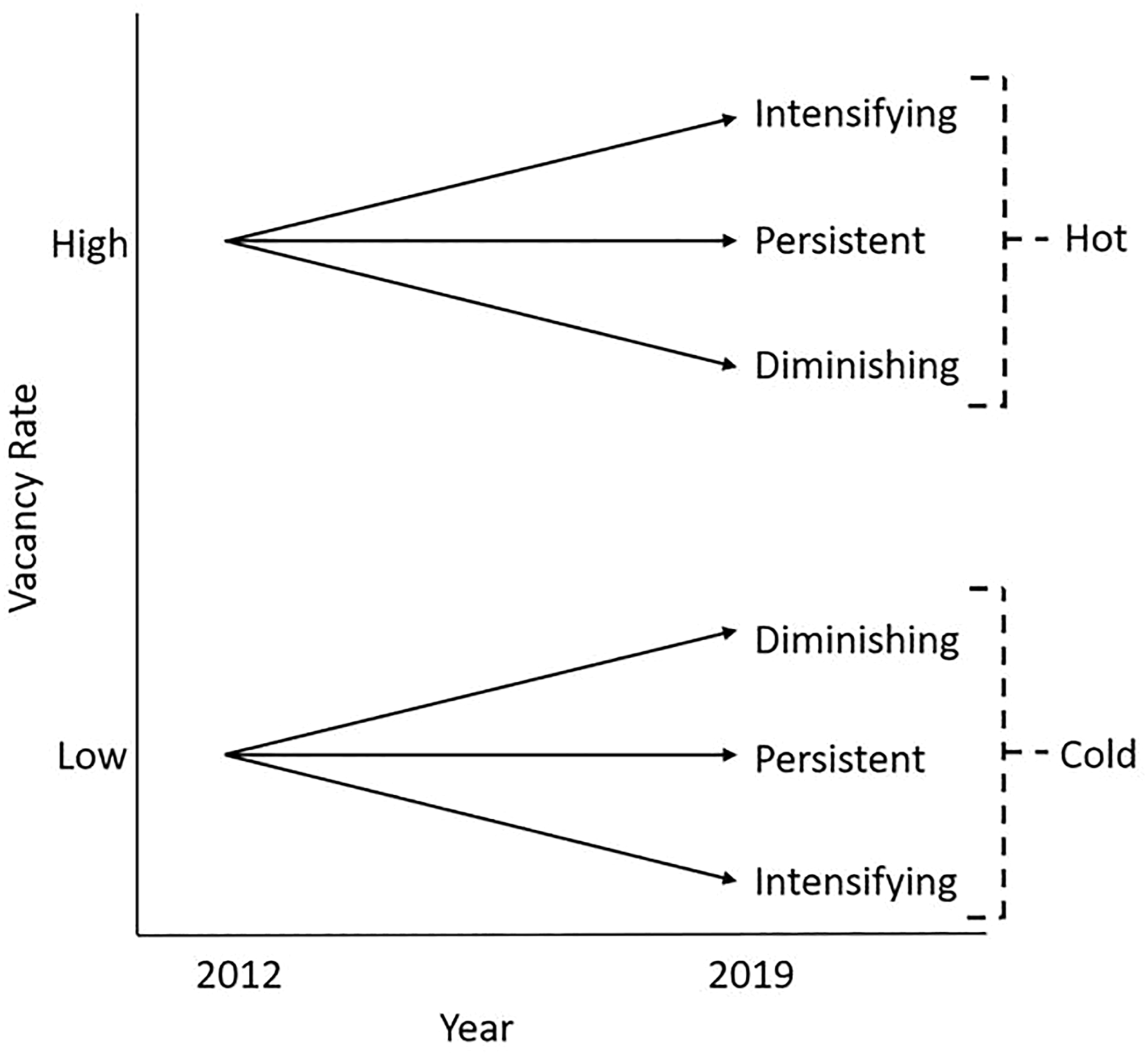
A schematic of emerging hot spot categories for vacancy rates.
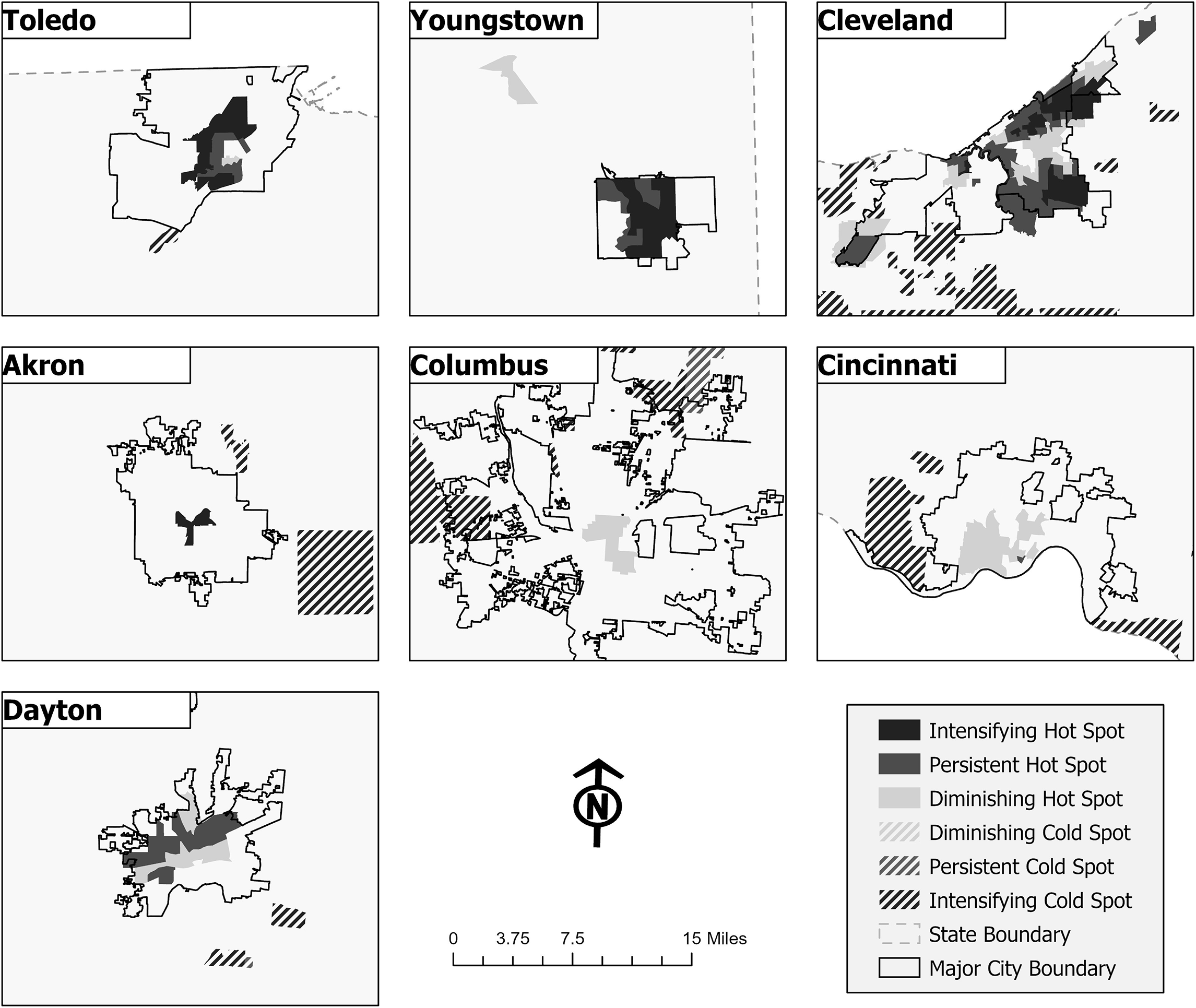
Emerging hot spot results for the seven largest MSAs in ohio.
Distribution of hot and Cold Spots by Ohio Metropolitan Statistical Area (MSA).

Notably, as part of the cube creation process, ArcGIS Pro automatically conducts another Mann-Kendall trend test that indicates whether the non-spatial trend for the variable of interest, across the entire study area (i.e. the state of Ohio), is statistically significant. In our case, vacancy rates in Ohio decreased over time (z = − 3.283, p = 0.001), which provides context for what we might expect at the MSA level. Given this statewide trend, if housing vacancy has no spatial pattern, vacancy should decrease everywhere in Ohio at the same rate. One could think of this as the null hypothesis.
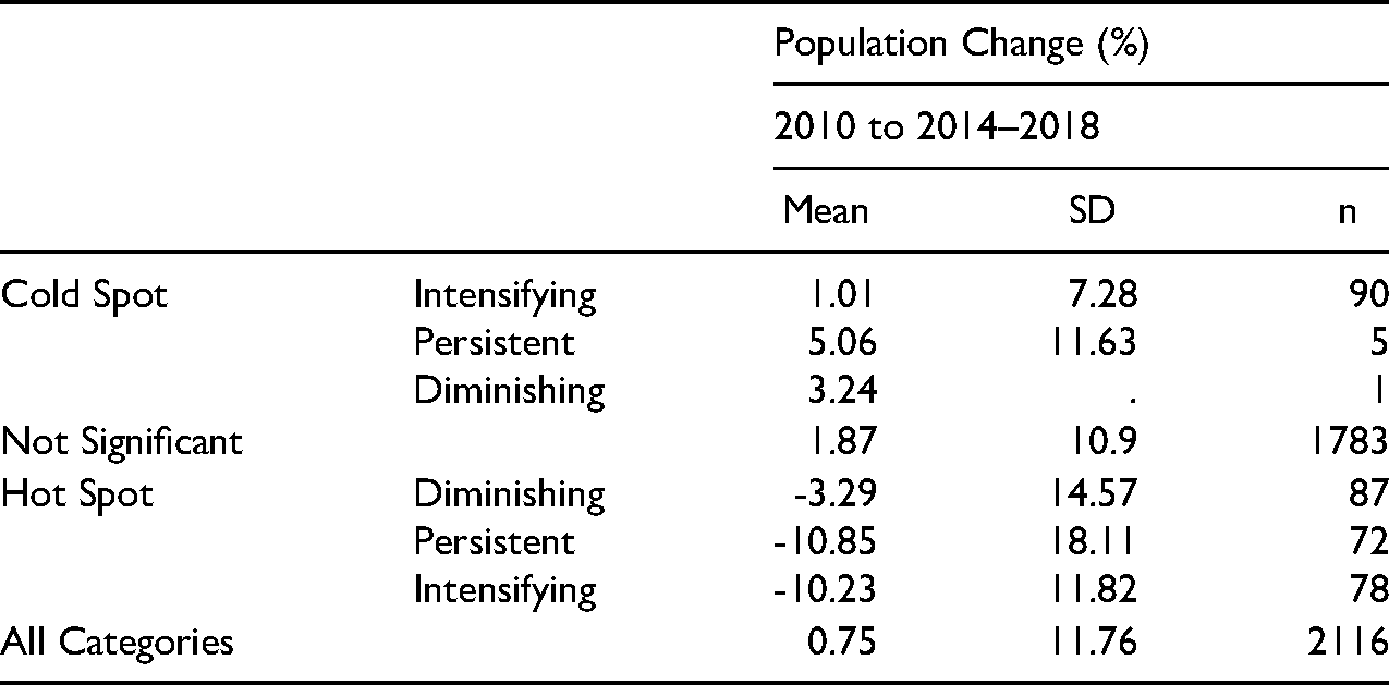
Population Data & Analyses: Once we identified emerging hot/cold spots per census tract for MSAs (in Table 2), we considered how population change at the tract, city, and MSA levels relate to the patterns of vacancy in Figure 2. To explore tract-level population dynamics, we used the 2010 decennial census and the 2018 5-Year American Community Survey (ACS) to calculate population change and run a one-way ANOVA with Games-Howell post hoc comparisons. 9 Because there is a time-lag between population losses and the emergence and identification of long-term vacancies (Reis, Silva and Pinho 2016), it is logical to have population estimates precede our vacancy estimates, particularly because the USPS does not classify units as vacant until mail is undeliverable for at least three months. The ANOVA tested for statistically significant differences in mean population change at the tract level between the hot/cold categories shown in Table 3, resulting in 15 unique comparisons. 10 In the next section, we report the statistically significant comparisons as well as the comparisons with results contrary to the expected pattern (i.e. a negative association between population and vacancy change).
Mean Population Change per hot Spot Category.
To explore the effects of the interaction of city and MSA population change on vacancy spread, we used the 2012 and 2018 1-Year ACS estimates to calculate population change and plot this change on an X-Y axis (Figure 3). Then, we compared the trends in Figure 3 to the emerging hot/cold spot results in Figure 2. For the MSA estimates, we aggregated county-level population data to the MSA level, to ensure estimates only included Ohio data. While this particular comparison is descriptive and cannot speak to statistical significance, clear visual patterns emerged between population dynamics at these higher scales (city and MSA) and vacancy at a lower scale (the tract), as we shall discuss in the next section.
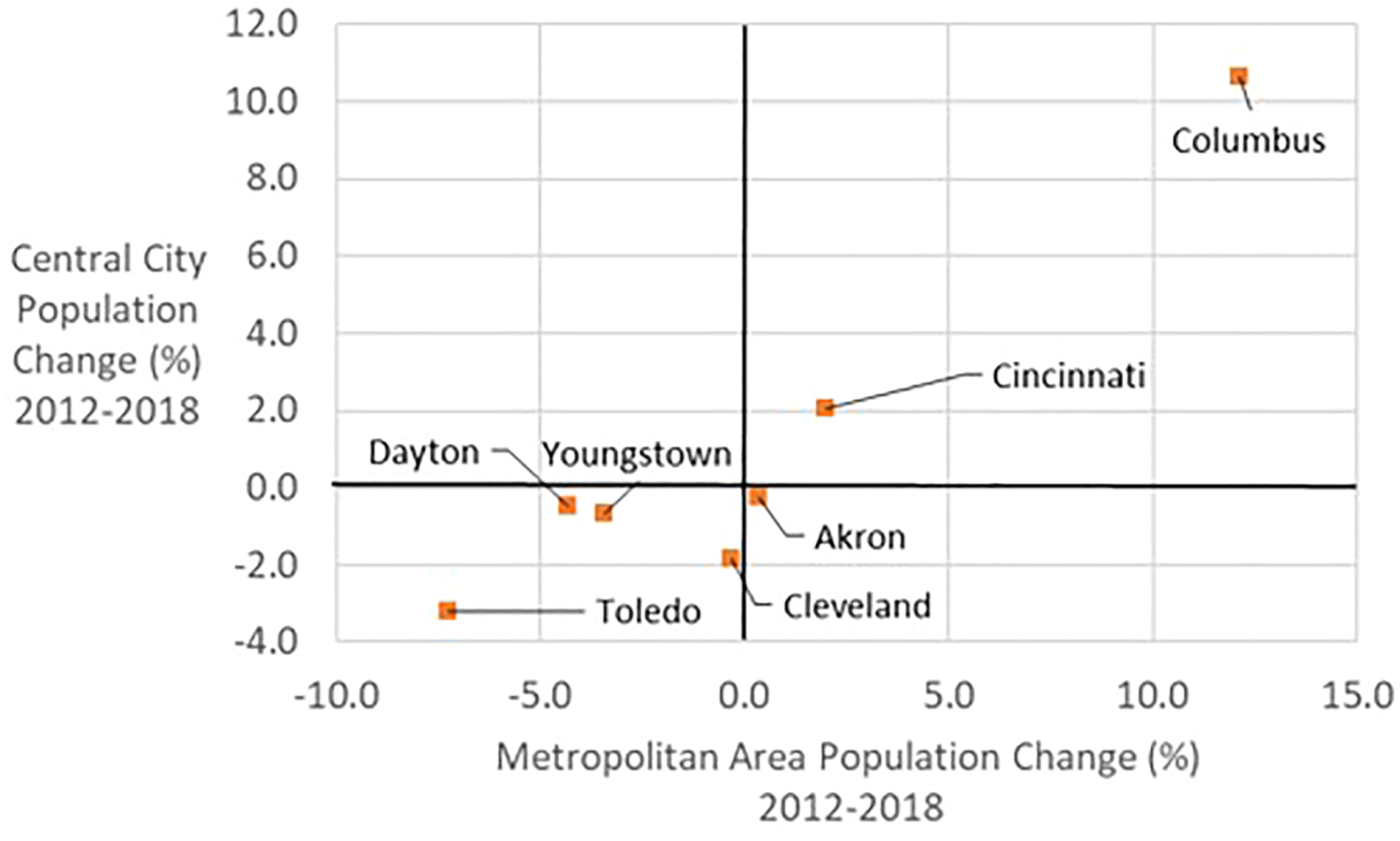
Population change by city and MSA, 2012-2018.
Results & Discussion
Spread of Vacancy: Our analyses demonstrate that housing vacancy does not spread in a uniform manner. The number and location of “persistent hot” and “diminishing hot” tracts vary within and between Ohio MSAs, as shown in Table 2 and Figure 2. Vacancy diminished in the cities of Columbus and Cincinnati, remained relatively high but stable in the city of Dayton, intensified in a small portion of the city of Akron and large portions of the cities of Toledo and Youngstown, and became polarized across the Cleveland MSA. Of the seven MSAs, the Cleveland MSA had the highest percentage of cold tracts, the highest percentage of hot tracts (when summing all three hot categories), and the lowest percentage of non-significant tracts. What is consistent across MSAs is that hot spots of vacancy are almost exclusively located in the central city, while cold spots are located outside of the central city. However, the hot spots were not always adjacent or circular in form, demonstrating that vacancy does not necessarily spread outward concentrically, though the relatively large size and irregular shape of tracts may account for some of the non-circularity.
Tract-Level Population Change: We also found a relationship between vacancy and tract-level population change. The ANOVA was statistically significant, indicating that the categories for the emerging hot spot analysis differed in their mean levels of population change [F(5, 2109) = 35.775, p < 0.001]. In general, cold tracts experienced population stability or growth, while hot tracts experienced population loss. Notably, the three cold categories, the not significant category, and the diminishing hot category did not statistically significantly differ from one another in their rates of population change (p > 0.05 for all comparisons), 11 though the diminishing hot category experienced average population loss. The rate of loss for the diminishing hot category also differed from the rate for intensifying hot (p = 0.012), and nearly differed from the rate for persistent hot as well (p = 0.055). 12
We expected population to increase on average for the diminishing hot category. However, if the rate of housing unit loss (e.g. demolitions) exceeds the rate of population loss, it is plausible for vacancy to decrease even though population continues to decrease. We briefly explored this possibility by examining tract-level housing unit change with the USPS dataset. Overall, average unit losses (of 3.91 percent) 13 across the study period exceeded the average rate of population loss (of 3.29 percent)—though for about a third of the diminishing hot tracts (35 of 87), population and units increased on average. 14 These findings suggest there are different types of tracts within the “diminishing hot” category, such as redeveloping tracts and tracts experiencing widespread clearance of vacant housing with no new development. However, given that the emerging hot spot methodology mathematically accounts for vacancy trends in neighboring tracts, it is plausible that some tracts may be classified as diminishing hot because of substantial improvements in adjacent tracts, and not significant decreases in vacancy within the tract itself. This possibility further emphasizes the practical and methodological importance of distinguishing between vacancy increase within a political unit and vacancy spread—that is, outward proliferation.
In general, we found that dramatic population declines correspond with neighborhoods with high but stable levels of vacancy and neighborhoods where vacancy is actively spreading. The persistent hot and intensifying hot categories had similarly high rates of population loss (at 10.23 percent and 10.85 percent across an 8 year period) that statistically significantly differed from the rates for the cold and not significant categories (p < 0.05 for all comparisons), but did not differ from each other (p > 0.999). Why both categories had similarly high rates of loss is not clear and worthy of future investigation.
City and MSA Population Change: By considering how the spatiotemporal patterns of vacancy (shown in Figure 2) differ by the interaction of population trends at the city and MSA levels (shown in Figure 3 and supported by Table 2), we found evidence of a relationship between tract-level vacancy and population change at scales higher than the tract. The cities of Columbus and Cincinnati, and their respective MSAs, are both growing. These cities are the only ones not experiencing persistent or intensifying vacancy at the tract level within our sampling frame. Vacancy in both cities’ cores diminished, with no corresponding increase elsewhere in the MSAs. The city of Akron and its MSA did not experience significant population change, and vacancy intensified in only a few small tracts near Akron's core. The city of Dayton's population is relatively stable, though it is losing population at the MSA level. Vacancy within that city is relatively high but stable, with a large percentage of tracts classified as persistent hot but none classified as intensifying hot. In contrast, the city of Youngstown fared considerably worse than Dayton, despite having similar population trends. Significant portions of Youngstown experienced vacancy spread (i.e. had tracts classified as intensifying hot) with no tracts in its MSA classified as cold. Cleveland experienced a decline in central city population and a slight decline in the population of its MSA—yet its vacancy pattern differed significantly from the other Ohio cities and MSAs, as noted previously. Cleveland has diminishing hot spots in close geographic proximity to intensifying hot spots, and a relatively large percentage of tracts outside of the city classified as hot or cold. In Toledo, where population decreased at both the city and MSA levels, vacancy spread in large portions of the central city, with only one tract classified as cold outside of the city.
Conclusion
We add to the limited number of tools available for measuring urban shrinkage by applying a newer method—emerging hot spot analysis—to the study of the spread of housing vacancy. We also demonstrate how ArcGIS Pro's auto-generated emerging hot spot results can be simplified to 7 ordinal categories, creating additional possibilities for subsequent, inferential analyses like ANOVA. These methods can be applied to a wide range of spatiotemporal phenomena.
In terms of our contribution to the housing literature, by using the aforementioned methodology, we found variation in the extent and location of the spread of housing vacancy within and between Ohio MSAs. In alignment with prior literature, vacancy spread in our study was most pronounced in central cities, particularly in shrinking cities located within shrinking MSAs. However, unlike prior literature that presumes a relatively uniform spread of vacancy from a cluster of vacant housing units (Morckel 2014b), we discovered that many Ohio MSAs concurrently experienced spread, contraction, and vacancy stabilization in tracts located adjacent to, or within close proximity of, one another. These results indicate that how vacancy proliferates is not solely a matter of geographic determinism, whereby high vacancy in one tract predicts high vacancy in neighboring tracts in future years.
While it is not novel to find an association between population change and vacancy, what is noteworthy is the potential relationship between vacancy spread at a small scale and population dynamics at much larger geographic scales. As such, our results run counter to much of the housing literature that theories vacancy as a neighborhood-level phenomenon (e.g., Morckel 2014b; Arsen 1992), and further suggests that initiatives intended to reduce vacancy (e.g. foreclosure prevention programs, demolition funding) should account for population trends in adjacent neighborhoods, the city as a whole, and the MSA—and not just physical conditions within a particular neighborhood. Two neighborhoods that are located in different contexts (different cities with different population dynamics) may not respond to the same vacancy reduction strategies, even if vacancy levels are comparable at the time of intervention.
Likewise, given our results, we suspect that property rehabilitation is more likely to reduce vacancy at all scales in growing MSAs versus shrinking ones. In accordance with the processes of housing filtering (Rosenthal 2014) and the “housing disassembly line” (Galster 2012) 15 rehabilitation in a shrinking MSA may merely shift vacancy elsewhere within the city or MSA, since the demand for newly rehabilitated homes is likely coming from within the MSA. Consequently, property rehabilitation in a shrinking MSA should probably occur in a geographically concentrated area, with the understanding that vacancy is likely to ensue elsewhere in the MSA because of the severe oversupply of housing relative to demand. This is not to say that rehabilitation should never occur in places that are losing population. Rather, we provide this example to emphasize how interventions at a local scale may exacerbate challenges at a higher scale (and vice versa), and why it is useful for policy makers to understand the multifaceted, interrelated nature of property vacancy and population change.
Our methodology and results also highlight a related topic that has received little attention in the literature: vacancy contraction (indicated by our “diminishing hot” category). As noted previously, we found that on average, tracts classified as diminishing hot experienced population loss. Given the competing explanations for this counter-intuitive relationship (discussed in the prior section), additional research is warranted on this phenomenon. The factors that drive vacancy contraction may not be the polar opposite of those that contribute to its spread.
We must also further emphasize the exploratory nature of our work, and how our contributions are primarily descriptive and methodological. This paper says more about patterns of shrinkage than it does about its causes. We do not argue that population loss is the sole cause of vacancy; rather, we conclude that vacancy operates differently from place to place and is associated with population dynamics at different scales. We fully recognize that the relationships found herein are likely influenced by a number of factors we did not control for (e.g. quality of code enforcement, level of demolition funding, degree of sprawl relative to central city size, quality of school districts, broad economic trends, number and types of employment opportunities available locally). We therefore invite others to further investigate why spatiotemporal patterns of vacancy substantially vary from place to place.
There may also be some question about how well our results generalize beyond Ohio. We suspect our findings are most applicable to post-industrial MSAs within the Midwest and Great Lakes regions that face similar population trends to Ohio MSAs, particularly ones with shrinking central cities. This study would be more generalizable with a larger sample, especially one that includes growing cities located within shrinking MSAs, and shrinking cities located within growing MSA—though this combination of population dynamics is rare in the United States (Ribant and Chen 2020) and was not present within our sampling frame. Moreover, while we generally focused on how vacancy spreads within MSAs at the tract level, similar questions can be asked at much smaller scales like the parcel or block (e.g. Does vacancy spread relatively concentrically at the parcel level? Why does vacancy spread from one block to another? Is block-level vacancy affected by city-wide population dynamics?).
In terms of temporal generalizability, our study may be most applicable to periods of economic expansion, since our date range represents a time of national recovery and declines in vacancy following the Great Recession and the late 2000s housing crisis. Repeating our study during a time of economic contraction (and possible widespread increases in vacancy) may be more illustrative of the ways in which vacancy spreads. If so—and if it is true that national economic trends matter to local levels of vacancy—this would further suggest an interaction effect at yet another scale (the national). It would also point to the importance of economic change in processes of shrinkage, consistent with much of the literature on urban decline in the American Midwest (Rhodes and Russo 2013).
Overall, our work adds to the methods available to measure shrinkage. It is an early contributor to a better understanding of the spatial patterns of vacancy proliferation and the relationships between population dynamics and city shrinkage. Because there is mounting evidence that grow-oriented urban planning strategies do not work in a context of shrinkage (Dewar and Thomas 2012), more research should be done on the physical manifestations of shrinkage such as housing vacancy. When combating neighborhood decline, researchers and practitioners should carefully consider concepts like Segers et al. (2020) “shrinkage in growth,” and what we might term “shrinkage in shrinkage” (i.e. shrinking neighborhoods located in a broader context of shrinkage). Urban planners and policy makers must view the city as an intricate system with interventions at one geographic scale potentially affecting all others.
Footnotes
Acknowledgments
The first author would like to thank Michigan State University's Urban and Regional Planning program for hosting her Fall 2019 sabbatical which made this publication possible.
