
Abstract
Recent systematic research indicated percent of the population that is young is not significantly associated with cross-national homicide victimization rates. However, there are theoretical reasons to expect percent young may be associated with 15 to 24 age-specific and with gender-specific cross-national homicide victimization rates. We test three hypotheses: Percent young is associated with 15 to 24 age-specific, male-specific, and female-specific homicide victimization rates. We employed data for 1999-2004 from a sample of 55 nations and utilized multiple statistical analyses. Results indicated no significant association between percent young and 15 to 24 age-specific and gender-specific homicide victimization rates. We situate our findings within the larger literature.
Keywords
Many scholars of violence, especially those who study cross-national variation in violence rates, believe there is an association between the proportion of a national population that is young (which we call “percent young” throughout, and usually defined as those in the age group of 15-24 years) and homicide rates. In spite of theoretical arguments and its regular inclusion in prior studies, however, Nivette’s (2011) meta-analysis and Trent and Pridemore’s (2012) review of cross-national homicide studies provided reasons to doubt this association. Furthermore, in a companion piece to the current study (Rogers & Pridemore, 2015), we systematically examined this association. We not only found no evidence of this association but our analyses also revealed that the inclusion of percent young in cross-national models of homicide damages model fit.
With a few exceptions, the research on the structural covariates (including percent young) of cross-national homicide rates has focused almost exclusively on total homicide rates. There are theoretical reasons to believe, however, that there may be differential effects of percent young on age-specific (especially on 15-24 age-specific) and gender-specific homicide rates. We explore these hypotheses here.
Literature Review
Compositional and contextual explanations are often justifications for including percent young as a variable in cross-national homicide models, and both theoretical approaches predict a positive association (Gartner, 1990; LaFree, 1999; Rogers, 2014; Rogers & Pridemore, 2015; South & Messner, 2000). There are two alternative theoretical arguments, modernization and differential engagement, but neither proposes a direct effect of percent young on homicide victimization across nations. The first alternative theory is the modernization argument, though studies of modernization typically include percent young as a part of a factor variable or principal component (Neuman & Berger, 1988; Ortega, Corzine, Burnett, & Poyer, 1992). This indicates the modernization approach does not expect a direct effect of percent young on cross-national homicide victimization rates but instead that the proportion of young people in a society is part of an underlying latent trait (modernization) expected to be associated with homicide rates. The second alternative theoretical explanation is differential engagement, in which the effect of percent young on homicide is conditioned on the lack of engagement of the young population (McCall, Land, Dollar, & Parker, 2013). This argument has only been explored with U.S. cities, however, and may not be applicable to a cross-national sample.
Although both the compositional and contextual approaches both expect a positive association between percent young and homicide victimization across nations, the theoretical mechanism explaining the association varies across the theories (Easterlin, 1987; Greenberg, 1985; Marvell & Moody, 1991; Pampel & Gartner, 1995). The compositional approach theorizes that the absolute size of the young population results in increased homicide victimization rates across nations (Gartner, 1990; Gartner & Parker, 1990; LaFree, 1999; Lafree & Tseloni, 2006; Pampel & Gartner, 1995) because the 15- to 24-year-old age group is believed to have the highest rates of violent offending and victimization (Gartner, 1990; LaFree, 1999; Ortega et al., 1992; South & Messner, 2000). Scholars often utilize the age–crime curve argument to explain why the young are most likely to be overrepresented as offenders (Gottfredson & Hirschi, 1990). The age–crime curve literature has argued that the youthful population will most often have the highest proportion of offenders across time and place (Gottfredson & Hirschi, 1990; Hirschi & Gottfredson, 1983; Marvell & Moody, 1991). That is, no matter the year or location (and this should include nations), it is expected that the youthful population will have the highest offending rates. While the reason why the youthful population is more likely to commit crime and become victims is debated (Blumstein & Nagin, 1974; Gottfredson & Hirschi, 1990; Greenberg, 1977, 1985; Hirschi & Gottfredson, 1983), most researchers agree that percent young is a driving mechanism for higher crime rates within and across nations (Chilton & Spielberger, 1971; Gartner & Parker, 1990; Greenberg, 1977, 1985; Hirschi & Gottfredson, 1983; Ortega et al., 1992; Pampel & Williamson, 2001).
Empirical support for the compositional argument is inconclusive (Nivette, 2011). Gartner and Parker (1990) explored homicide and age across a small sample of nations without specifically addressing the association of age past the percent of the total population 15 to 34 years of age. They found that there was unlikely an association between age and homicide in Scotland or Japan, but possibly an association post-World War II in the United States and Italy. This is one of the few studies that graphed age-specific homicide rates over time within nations, though the authors did not formally test for an association between percent 15 to 34 and homicide victimization rates within nations. Gartner (1990) did also examine within-nation effects for some nations and found that age appeared to have a significant association with homicide within but not across nations. These results for tests of a direct effect of age on homicide are inconclusive, and a more in-depth discussion of the varieties of findings appears later in the literature review. However, to date there are more studies that find a nonsignificant association with homicide and percent young than there are that find the predicted positive association (for reviews of the literature see Nivette, 2011; Pridemore & Trent, 2010; Rogers & Pridemore, 2015; Trent & Pridemore, 2012).
The contextual approach theorizes that a large birth cohort creates conditions that will increase the likelihood that members of the birth cohort will be either offenders or victims (Easterlin, 1987; Rogers & Pridemore, 2015; South & Messner, 2000) due to competition for scarce resources. This explanation is most associated with the work of Easterlin (1987). This approach suggests that the negative outcomes that arise from being born into a large birth cohort are what cause the youthful population to have higher offending and victimization rates. There is some indirect support for this theoretical argument. For instance, in the post-WWII years in nations that observed a “baby boom” there were increased homicide rates (Gartner & Parker, 1990). In addition, the negative consequences of large birth cohorts have been found to have some association with homicide victimization across nations. These correlates such as poverty (Messner, Raffalovich, & Sutton, 2010; Paré & Felson, 2014; Pridemore, 2008, 2011) and lack of social capital (Altheimer, 2008; Knack & Keefer, 1997; Lederman, Loayza, Menendez, & Menendez, 2001) have been found to be significantly associated with homicide across nations. However, there have been no direct formal tests of this theory and often it is only discussed as a by-product of what could possibly explain why the variable for the percent young should be included as a control variable (South & Messner, 2000).
No matter the approach utilized to justify including percent young, it is expected to be positively associated with homicide victimization rates across nations (Easterlin, 1987; Greenberg, 1985; Pampel & Gartner, 1995; Pampel & Williamson, 2001). Our recent systematic and extensive analyses, however, did not support these statements (Rogers & Pridemore, 2015). Our analyses consistently failed to reject the null hypotehsis of no association between percent young and cross-national homicide victimization rates and found that inclusion of percent young in a statistical model of cross-national homicide rates results in overfitting the model, which damages prediction models due to increases in the errors when estimating coefficients (Hocking, 2003; Myers, 1990).
Age-Specific Homicide Victimization Rates
Despite these findings for total homicide rates it may still be that percent young is significantly associated with age-specific or gender-specific homicide victimization rates. For example, Wolfgang (1967) observed that homicide victims and offenders were often of similar ages, with offenders being slightly younger than victims. More broadly, as the compositional theory proposes that the young are more likely to be violent victims and offenders (Butchart, Engström, & Engstrom, 2002; Chilton & Spielberger, 1971; Cohen & Land, 1987; Fiala & LaFree, 1988; Greenberg, 1985; Marvell & Moody, 1991), the expectation is that the 15 to 24 age-specific homicide victimization rate would also be larger because they are expected to be the most likely to be victimized by those of similar age.
Few studies have explored cross-national age-specific homicide victimization rates (for reviews, see LaFree, 1999; Nivette, 2011; Rogers & Pridemore, 2015; Trent & Pridemore, 2012). Studies that did examine age-specific rates found that some variables had different associations with the different age-specific rates (Butchart et al., 2002; Moniruzzaman & Andersson, 2005). In this small literature, the majority of studies examined the differential effects of economic inequality on age-specific homicide victimization rates, with findings revealing that the impact of inequality on homicide rates was stronger for younger populations (Butchart et al., 2002; Moniruzzaman & Andersson, 2005). Thus, theory and research on other structural covariates suggests percent young may affect 15 to 24 age-specific homicide victimization rates differently compared with its null effect on the overall homicide victimization rates across nations.
Gender-Specific Homicide Victimization
There are also reasons to expect percent young may differentially affect gender-specific homicide victimization rates. Agha (2009) explored if the correlates of cross-national male homicide victimization also explained female homicide victimization. While the overall conclusion was that the structural covariates of male and female homicide victimization rates were generally similar, the models did a poorer job explaining female homicide victimization rates (i.e., they had a smaller adjusted R2). Another notable exception is Stamatel’s (2014) exploration of variation in female homicide victimization across European nations. The common theoretical explanations employed to explain variation in homicide victimization did not perform as expected when attempting to account for female homicide victimization. Both of these previous studies provide support for the need to explore correlates of both male and female homicide victimization separately. Moreover, within the U.S. homicide literature there is a larger body of empirical research exploring the correlates of male and female homicide victimization. Overall, this literature finds that in some instances there are different correlates of gender-specific homicide victimization (in the United States: Schwartz, 2006; across U.S. cities: Smith & Brewer, 1992). Therefore, both to be sensitive to these potential differences and to be as systematic as possible in our exploration of this possible association we will test if the association between percent young is different for male and female homicide victimization cross-nationally.
There are theoretical reasons to question if percent young affects male and female homicide victimization rates differently across nations. The contextual approach proposed by Easterlin (1987), the negative outcomes associated with large birth cohorts, is gendered. The vast majority of these outcomes, as Easterlin discussed them, should have negative effects on males more than females. Taking into account Easterlin’s arguments it would seem imperative to ensure a systematic exploration of the association between percent young and both female and male homicide victimization rates cross-nationally.
Hypotheses
The literature indicates there is likely no association between percent young and total homicide victimization. However, this may not be true for percent young’s impact on 15 to 24 age-specific or on gender-specific homicide victimization rates. Therefore, we test three hypotheses that will aid in understanding the efficacy of percent young (either as a theoretical variable of interest or as a control variable) in cross-national homicide research. The three hypotheses are as follows: Percent young is associated with (a) 15 to 24 age-specific, (b) male-specific, and (c) female-specific homicide victimization rates.
Data and Method
Sample
The sample consists of 55 nations, which are listed in the appendix. The majority of the sample is from Europe. While this is a limitation, we attempt to adjust for this oversampling of Europe by including regional control variables in our models.
The sample size is limited because of the sources of data we are employing to measure the variables of interest. Within the recent cross-national homicide literature there have been larger sample sizes, but this may very well come at the cost of validity. Specifically, there are limitations with using a mixture of victimization and offending rates and there are serious limitations with using homicide data from police and United Nations. A key limitation of the former is that offending and victimization may not have the same correlates, which is an important point often ignored by criminologists. The two are not necessarily interchangeable. The source of data is also important when trying to limit measurement errors. For police registries and UN homicide rates (both of which are based on offending) there are differences in definition of homicide, differences in reporting practices, and other limitations that add to the measurement error (for a richer discussion, please see Smit, de Jong, & Bijleveld, 2012; Smit, Meijer, & Goroen, 2004).
Data
The outcome variables are (a) 15 to 24 age-specific and (b) gender-specific homicide victimization rates for 1999 to 2004. If data were missing for any years, we ignored the missing years in the average. The nation with the most missing years was Georgia (missing 2002-2004). Seven other nations had one missing observation throughout the 5-year time span: Armenia (2004), Australia (2004), Hungary (2003), Italy (2004), Portugal (2004), Puerto Rico (2004), and Uzbekistan (2001).
We obtained homicide victimization and population data from the World Health Organization’s Statistical Information System (WHOSIS) database (World Health Organization, 2012). Homicide is defined using the International Classification of Diseases 10th revision categories X85-Y09 (World Health Organization, 2012), that is, “homicides and injury purposely inflicted by another person.”
The key independent variable was the percent of the entire population aged 15 to 24 years. The 15 to 24 age group is most often used within the recent empirical cross-national homicide literature as the definition of young. The total population within the age group and the total population within nations were obtained from the WHOSIS database (World Health Organization, 2012).
Control variables included sex ratio (males per 100 females), infant mortality rate (infant deaths per 1,000 live births) as a proxy for poverty, total population, Gini coefficient of income inequality, the education component of the Human Development Index, unemployment rate, percent of the population living in urban areas, crude divorce rate, gross domestic product (GDP) per capita, ethnic heterogeneity, and regional controls (using the regions as defined by the World Health Organization). These variables are included in our models based on the previous empirical cross-national homicide literature (for an overview of the theoretical reasons for including these variables see Nivette, 2011; Trent & Pridemore, 2012).
Analyses
We utilized multiple statistical estimation techniques to test the hypotheses. The first was ordinary least squares (OLS). We constructed the models such that variables were introduced based on sample attrition due to missing data. Therefore, initial models included all variables without missing data and each variable was then included based on the number of nations lost in the sample due to missing data. It is possible that percent young will matter in certain samples or with specific variables, and the stepwise process allowed us to explore this possibility.
The next analysis utilized the sequential ANOVA to test the association between percent young and homicide rates. 1 A sequential ANOVA provides information regarding the unique contribution of a variable given the variables included in the model before it. The sequential ANOVA is also helpful when multicollinearity is present. This allows for a slightly different view of the relationship between percent young and age- and gender-specific homicide rates. By changing the order in which variables are introduced into the sequential ANOVA it is possible to test the unique contribution of a variable net of the effect of any variable it is highly correlated with, and therefore is one way to see how much multicollinearity affects the OLS model.
The third set of techniques included two model comparison methods, the likelihood ratio test (LRT) and the Wald Test (Agresti & Finlay, 2008), which test if the variable omitted from the reduced model significantly aids in accounting for the variance in homicide rates by reducing the error in the projection of the regression line. It is not common practice to explore the t statistics in the statistical output, despite the t statistic providing information beyond that of being a test statistic for the beta coefficient. The resulting F statistic from the Wald Test is the t2 statistic for the removed variable.
The final estimation technique is Mallows’s Cp, a more precise method of model selection (Mallows, 1973) that allows measurement of model over- and underfit. The value obtained during Mallows’s Cp (i.e., the Cp) estimation is a ratio of bias-to-variance. Having too few variables in the model that contribute to explaining the variation leads to underfit, which biases the model. Having too many variables in the model and including variables that do not contribute to explaining the variation results in overfit, which introduces more variance into the estimation of the outcome. To estimate Mallows’s Cp we used an initial model that included percent young, poverty, total population, ethnic heterogeneity, sex ratio, Gini coefficient, the education index, and unemployment. The region controls are removed because Mallows’s Cp cannot be estimated with multiple dummy control variables (Hocking, 2003).
Results
Descriptive Statistics
The distributions of 15 to 24 age-specific, male-specific, and female-specific homicide victimization rates, and of percent young, poverty, total population, GDP, and the Gini coefficient were not normal according to the Shapiro–Wilk, boxplots, quantile-quantile (QQ) plots, and Box-Cox transformation diagnostic tests. A natural log transformation was utilized to attempt to make these distributions approximately normal. Finally, ethnic heterogeneity and crude divorce rate were transformed using the square root to make them approximately normal according to the Shapiro–Wilk, boxplots, QQ plots, and Box-Cox transformation diagnostic tests.
Table 1 provides the correlation matrix and the means and standard deviations for all variables (including those that were transformed). Percent young (r = .67), poverty (r = .71), and ethnic heterogeneity (r = .61) were all positively and significantly correlated with the 15 to 24 age-specific homicide victimization rates. Male and female homicide rates were strongly correlated (r = .88). Percent young was correlated with male (r = .73) and female homicide rates (r = .56).
Correlation Matrix and Descriptive Statistics.

Note. Boldfaced values indicate p < .05.
OLS Model Estimation
Table 2 provides the OLS results for the stepwise models with the outcome for the 15 to 24 age-specific homicide victimization rates. 2 Due to space limitations, the reduced models (i.e., those that remove percent young from the model) are not shown in Table 2, though model fit statistics are provided within the table for both the full and reduced models. 3
Stepwise Models for Percent Young’s Effect on 15 to 24 Age-Specific Homicide Rates.

Note. Region controls were included but results are suppressed due to space constraints. The comparison group is Eastern Europe. “Full” indicates full model (i.e., includes percent young) and “reduced” indicates percent young was excluded from the model. Standardized beta within parentheses. MSR=Mean squared residuals. Boldfaced values indicate p < .05.
The results are the same for all of the models exploring the association between percent young and the 15 to 24 age-specific homicide victimization rates. Across all seven of the full models, percent young was never significantly associated with the 15 to 24 age-specific homicide victimization rates across nations. Moreover, across all models, the R2 and adjusted R2 statistics remain relatively similar, and in Models 5 and 7 there was no change in the adjusted R2. No change or little change in the R2 and adjusted R2 is indicative of a variable having little to no effect on the outcome variable. This is likely an indicator of overfitting the model, as a variable that accounts for little to no variation in the outcome is not contributing to the overall model and may be hindering it by increasing the error in estimation.
To further test the idea that percent young may be hindering the ability to account for variation in 15 to 24 age-specific homicide victimization rates, and thus damaging model fit, we conducted likelihood ratio (LRT) and Wald tests. The results are shown at the bottom of Table 2. These tests compare the full models presented in Table 2 with the reduced models that exclude percent young. The LRT and Wald tests indicate that across almost all of the models percent young does not aid in accounting for variation in 15 to 24 age-specific homicide victimizations. The one exception is for the LRT test for Model 6, and in a few models the test statistics for percent young were nearly significant.
Table 3 provides the results for the OLS models estimated with the outcome of male homicide victimization, percent young, and all of the control variables introduced in the same stepwise process as was done for the 15 to 24 age-specific homicide victimization models. 4 The results for the OLS models with the outcome of male homicide victimization are less conclusive. Percent young is not associated with male homicide victimization at a level of p < .05, though in Models 10 and 13 p = .051, and Models 8, 9, and 11 all would be significant if the p value requirement were p < .10. However, what is troubling for these models can be found within the model fit statistics at the bottom of Table 5. Across Models 8, 9, and 10, the R2 does not change. For each additional variable added, the R2 is expected to increase, and removing a variable should reduce the R2 statistic. There is a slight change when percent young is removed, but as with all models presented in Table 3 these differences are negligible. Moreover, the F statistic for model fit appears strong across all of the models that remove percent young, indicating that without percent young the model better accounts for male homicide victimization rates across nations. The results of the model fit statistics indicate that including percent young may be damaging model fit in a way that increases the amount of error in the estimation.
Stepwise Models for Percent Young’s Effect on Male Homicide Rates.
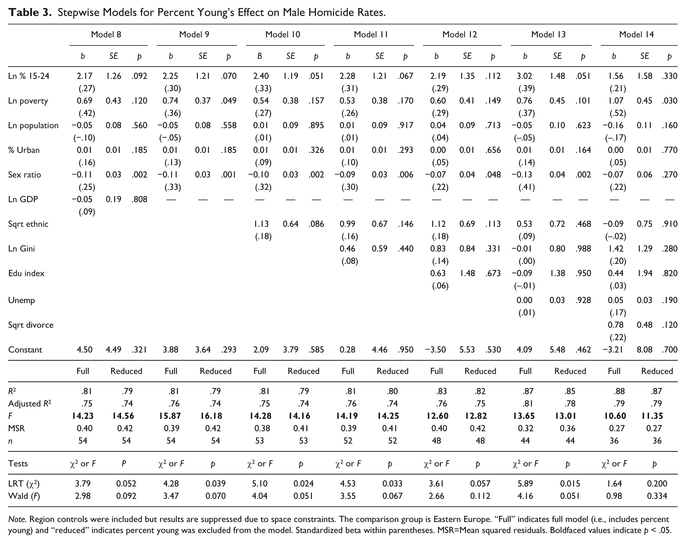
Note. Region controls were included but results are suppressed due to space constraints. The comparison group is Eastern Europe. “Full” indicates full model (i.e., includes percent young) and “reduced” indicates percent young was excluded from the model. Standardized beta within parentheses. MSR=Mean squared residuals. Boldfaced values indicate p < .05.
Table 4 shows results for the OLS models estimated with the outcome of female homicide victimization. Once again, the reduced models (i.e., those that exclude percent young) are not included in the table but the model fit statistics are provided. 5 The conclusion across all of the models is that percent young is not associated with female homicide victimization. Furthermore, the R2 and adjusted R2 values remain the same despite the inclusion or exclusion of percent young. Moreover, across all models the F statistic of model fit is better for the models that exclude the percent young.
Stepwise Models for Percent Young’s Effect on Female Homicide Rates.

Note. Region controls were included but results are suppressed due to space constraints. The comparison group is Eastern Europe. “Full” indicates full model (i.e., includes percent young) and “reduced” indicates percent young was excluded from the model. Standardized beta within parentheses. MSR=Mean squared residuals. Boldfaced values indicate p < .05.
The bottom of Table 3 presents the results of the likelihood ratio and Wald tests for both male victimization models. The same conclusions are drawn for all male homicide victimization models (Models 8-14). The LRT indicates that percent young may aid in accounting for male homicide victimization across nations but the Wald test, which is a more exact test as it strictly follows the F-distribution, indicates that across most of the models percent young does not aid in accounting for variation in male homicide victimization across nations. The bottom of Table 4 presents the results of the LRT and Wald test for all of the female models. Across all of the LRT and Wald tests for females (Models 15-21) percent young does not aid in accounting for variation in female homicide victimization across nations.
Sequential ANOVAs
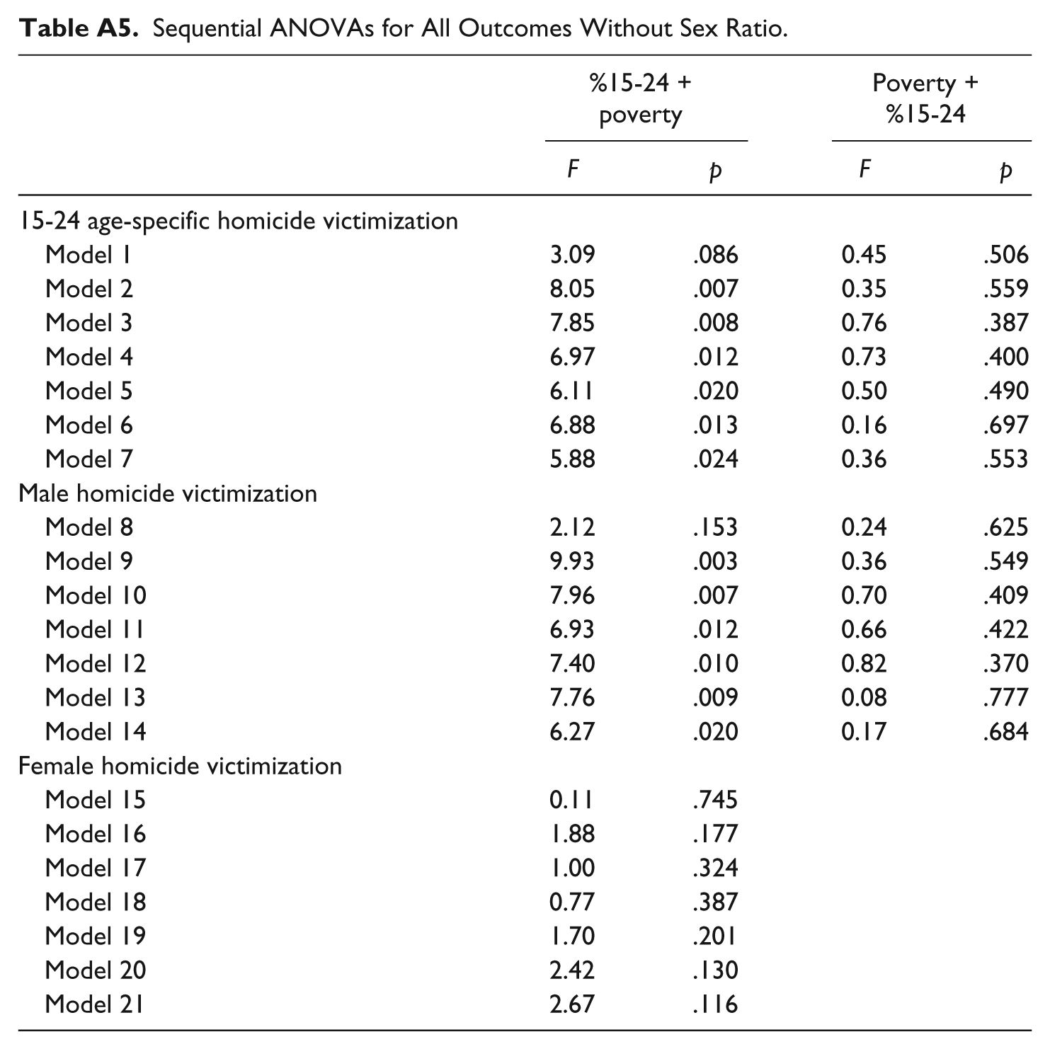
Table 5 provides the results of the sequential ANOVAs for the 15 to 24 age-specific, male, and female homicide victimization models. In those models in which percent young did not account for a significant proportion of the variance in the outcome variable we did not include the estimate for the second model (which includes poverty before percent young) because the results would be redundant showing percent young does not account for a significant proportion of the variance of the outcome variable being studied in the model.
Sequential ANOVAs for All Outcomes.

Note. The F statistics and p values are for the percent of the entire population aged 15 to 24 years.
The results are conclusive. For the 15 to 24 age-specific and male homicide victimization models, when percent young was included before poverty it usually accounted for a significant proportion of the variance in the outcome variables. However, when poverty is included before percent young, poverty accounted for all of the variance for which percent young otherwise would have accounted. This means that when poverty is included in a model percent young becomes a redundant variable. In addition, across all of the models that included percent young before poverty, poverty still accounted for a significant proportion of the variance despite whatever variance percent young accounted for, meaning poverty still matters despite the inclusion of percent young. Finally, the sequential ANOVAs for female homicide victimization all indicated that percent young did not account for a significant proportion of the variance in female homicide victimization. These tests all indicated that by including percent young we are overfitting the statistical model and increasing the error in the estimations. In other words, the inclusion of percent young damages model fit.
Mallows’s Cp
Model selection should be the first step in the model estimation process. However, previous research often found reason to include all the variables within the models estimated in the above section and reviewers often insist that each of the variables be included in cross-national homicide victimization models. Model selection is important in understanding the variances and bias trade-off that is the epitome of hypothesis testing in statistics, though, and can be partly understood through underfitting and overfitting statistical models. Here we use Mallows’s Cp to examine model fit, and if necessary we use R2 and adjusted R2 when multiple models fit the criteria for the Mallows’s Cp best model.
For the 15 to 24 age-specific homicide victimization models the best model according to Mallows’s Cp was a model that included poverty, percent urban, ethnic heterogeneity, the Gini coefficient, and the unemployment rate. This model’s Mallows’s Cp = 4.41, and therefore the model was slightly underfitted. However, when observing the adjusted R2 and R2 there were only incremental increases for the R2, and the adjusted R2 decreases, with each additional variable added to the model. Therefore, the best model for accounting for variation in the 15 to 24 age-specific homicide victimization rates across nations would be a model that does not include percent young.
The male homicide victimization model selection indicated that a six variable model was the best model. The Mallows’s Cp is 6.08, which means the model was slightly overfitted. The variables were poverty, population, percent urban, ethnic heterogeneity, Gini coefficient, and unemployment. The R2 for the models before were smaller and the R2 for the models afterwards increase negligibly (only to the fourth decimal point), and the adjusted R2s for the models before and after this model were smaller. Therefore, the best model for accounting for variation in cross-national male-specific homicide victimization rates is a model that does not include percent young.
Finally, for all of the possible combinations of the variables in the model (percent young, poverty, total population, percent urban, ethnic heterogeneity, Gini coefficient, education index, and unemployment) none of these resulted in a best fit model when the outcome variable was the female homicide victimization rate. For all the possible combinations of the variables and models, none resulted in a model fit that had a Mallows’s Cp equal or within the range of the number of variables in the model. The adjusted R2s for some models were also negative. This means these are poor models for explaining cross-national female homicide victimization rates.
Sensitivity Analyses
The first set of sensitivity analyses explored outliers and influential observations within the models using dfbeta, dffit, covariance ratio, Cook’s distance, and the diagonal of the hat matrix. 6 For the 15 to 24 age-specific homicide victimization rates, when the outliers were removed from Models 1, 2, and 3, percent young was significantly associated with the outcome. The male homicide victimization models showed significant positive associations between the percent young and male homicide victimization. However, all significant positive associations between percent young and the outcomes 15 to 24 age-specific and male homicide victimization rates became nonsignificant when sex ratio was removed from the models. After removing the outliers, percent young was not significantly associated with female homicide victimization rates.
The second set of sensitivity analyses reestimated the sequential ANOVAs when the outliers were removed from each of the models. Across each of the models, the same conclusions were drawn. In the sequential ANOVAs with 15 to 24 age-specific and male homicide victimization rates as the dependent variables and that included percent young before poverty, percent young resulted in significant contributions to accounting for variation within homicide. However, if the order was reversed and poverty was included in the model before percent young, percent young no longer significantly contributed to accounting for variation within homicide. Once again, despite removing outliers or changing the order in which percent young is included, percent young never uniquely accounted for a significant proportion of the variance in female homicide victimization rates.
Overall, there are some differences when the outliers removed for the 15 to 24 age-specific and male homicide victimization models. However, the results do not hold when sex ratio is removed from the model. Without sex ratio was included in the statistical models percent young was not associated with 15 to 24 age-specific or male homicide victimization. In addition, the proxy measure for poverty, with or without outliers, accounts for all of the variation that percent young accounts for and then some when the outcomes are 15 to 24 age-specific or male homicide victimization. Percent young never accounts for a significant portion of the variance in female homicide victimization. Therefore, by including percent young researchers are not gaining any additional ability to account for variation in 15 to 24 age-specific or gender-specific homicide victimization rates.
The third sensitivity analyses we employed addressed sample size and the possibility that by having a small sample size we may not have enough power to reject the null hypothesis. To test the power of the models we utilized an ad hoc power analysis for multiple linear regression. Specifically, we calculated the effect size of each model and then utilized the effect sizes to estimate lambda. Once we estimated lambda, we were able to use the distribution function (pf) in the R statistical package to obtain the final power values. For each model, power ranged from 0.95 to 0.99. The lowest power was observed for the last two models in Tables 2, 3, and 4. To be thorough, we also calculated the required sample size to obtain a power of 0.95, which showed that required sample sizes ranged from 20 to 31 nations.
The fourth set of sensitivity analyses explored both the partialling fallacy and the possible limitation of overfitting the models with the sheer number of variables we included in each model. 7 We employed principal components analysis (PCA) and compared scree plots, Eigenvalues, and the cumulative proportion of variation to deduce the required number of components to adequately capture the variation in the variables in each model (with the exception of percent young). These results suggested the use of two components for the first five models in each table (Models 1-5, 8-12, and 15-20), three components for the sixth model in each table (Models 6, 13, and 20), and four components in the seventh model (Models 7, 14, and 21) in each table. Finally, we reestimated every model (including the sequential ANOVAs) for each outcome and included percent young and the components from the PCA. The overall conclusion was that percent young does not have a significant association with 15 to 24 age-specific, male, and female homicide victimization. Percent young was significantly associated with homicide victimization in only four models (i.e., in only 19% of the 21 models we estimated). Moreover, in the four models where percent young was significantly associated with the outcomes, when sex ratio was removed from the PCA (and the models reestimated) percent young was no longer significantly associated with the outcomes (15-24 age-specific, male, and female homicide victimization).
The final set of sensitivity analyses explored the possibility of posttreatment bias. This is a common limitation in the cross-national homicide literature. Reviews of the literature show a wide array of variables deemed necessary as control variables whether or not there is sufficient evidence to suggest that the variable accounts for variation in both the outcome and predictor variables. There are a handful of ways to address posttreatment bias. The first is to explore the models to ensure each control variable included has an effect and there is a strong theoretical explanation for its effect on both the predictor and outcome variables. In doing this, we can state that each of the economic health variables (i.e., proxy for poverty, GDP, and Gini coefficient of income inequality) is expected to affect the predictor variable, percent young. This is established by the demographic transition literature (see Caldwell, 1976; Caldwell, Caldwell, Caldwell, McDonald, & Schindlmayer, 2006; Myrskylä, Kohler, & Billari, 2009) and in the globalization/nation development literature (see Gustaffsson & Johannson, 1999; Moller, Huber, Stephens, Bradley, & Nielsen, 2003; Smeeding, 1989; Smeeding, Torrey, & Rein, 1988). We also know that these economic health variables are often found to be associated with the outcome variable, homicide victimization rates (see Nivette, 2011; Trent & Pridemore, 2012). Therefore, we reestimated the models including only the percent young and one of the economic health variables discussed above and we arrived at similar conclusions. As long as an economic health variable is included, percent young is not associated with age- or gender-specific homicide victimization rates. We further explored if including or excluding other variables mattered and the conclusions remained the same with the exception of some of the models including sex ratio. This indicates that percent young is likely not performing as the previous literature has theoretically stated. It is more likely that percent young is acting as a measure of economic health (likely a proxy, given the discussion in the demographic and globalization/nation development literature).
Discussion
We tested three hypotheses to systematically explore if the percent of the entire population that is young has an effect on either 15 to 24 age-specific homicide rates or gender-specific homicide victimization rates. We did not find support for the hypotheses. While theory makes it necessary to tests these hypotheses, our findings are not surprising given the results from our recent study of percent young and overall homicide rates that led us to consistently fail to reject the null hypothesis of no association between the two but also that the inclusion of percent young damages model fit (Rogers & Pridemore, 2015).
In addition to the earlier study these new analyses utilizing 15 to 24 age- and gender-specific homicide victimization rates provide multiple unique contributions to the cross-national homicide literature. Our first contribution is an additional test of the compositional theoretical statements as they relate to age and homicide cross-nationally. This approach posits percent young will have a significant positive association with age-specific and gender-specific homicide victimization rates across nations. While our prior study of overall homicide rates provided reason to doubt any association between percent young and homicide victimization across nations, the present study allows us to state with greater confidence that percent young likely does not contribute to accounting for a significant proportion of the variance in cross-national homicide victimization rates (whether overall, 15-24 age-specific, or gender-specific). In addition, by including percent young researchers are overffiting their statistical models and increasing the variance in their estimates. In short, we do not find support for the compositional argument no matter the outcome variable employed in the analyses.
The next significant contribution that we make to the literature is an attempt to open discussion regarding the possibility that there may be different correlates of female homicide victimization compared with overall and/or male homicide victimization rates. As noted, the R2 and adjusted R2 for the female homicide victimization models are small, and in some cases during the Mallows’s Cp model selection process there were negative adjusted R2s. There are two possible reasons behind these small and sometimes negative adjusted R2s. The first is that there is simply not enough variation in female homicide victimization across nations to account for, and therefore the R2s are small. Alternatively, it is possible that what accounts for variation in male homicide victimization rates will not account for much, or any variation, in female homicide victimization rates. Future research should explore these possibilities.
Our final main contribution is to address the importance of model selection in cross-national homicide research. Overfitting or underfitting a model is detrimental to researchers’ understanding of a phenomenon because (a) overfitting increases the error in the estimates of the effects of the variables on homicide victimization and (b) underfitting biases results. As part of building models to understand homicide victimization across nations, it is important to balance the statistical models utilized so that the models are parsimonious and allow for a test of theoretical arguments. It is also possible to test theoretical statements using these model selection techniques. For example, if a theory suggests a particular should be extremely important in explaining homicide victimization across nations and yet model selection techniques like Wald’s Test, LRT, or Mallows’s Cp indicate the variable does not aid the model, then it is unlikely that the theory or variable is accurately explaining homicide victimization rates across nations.
15 to 24 Age- and Gender-Specific Homicide Victimization
The first hypothesis was that percent young would have a significant association with 15 to 24 age-specific homicide victimization rates. The second and third hypotheses were that percent young would have a significant association with male- and with female-specific homicide victimization rates. Multiple OLS models revealed a consistent lack of support for all three hypotheses, and additional analyses—including sequential ANOVAs and Mallows’s Cp—similarly did not support the inclusion of percent young as a predictor and/or control variable in the cross-national homicide models. These consistent findings spanned differences in sample composition, sample size, and the variables included in the model.
There are some minor deviations in which it is possible with a larger sample (thereby increasing the power of the models) percent young may have had a significant association with 15 to 24 age-specific and male homicide victimization rates. However, even within the models where percent young was approaching significance, when sex ratio was removed from the model percent young was no longer significant. The sequential ANOVAs helped provide insight into this limitation of the analyses and suggested exclusion of percent young from the models.
To some our findings may be surprising given the (a) inclusion of percent young in many cross-national homicide studies, (b) theoretical arguments for an association between percent young and cross-national homicide rates, and (c) insistence of many reviewers that percent young be included in studies of cross-national homicide rates. On the other hand, our findings should not be surprising given results of several prior studies (Gartner, 1990; Nieuwbeerta, McCall, Elffers, & Wittebrood, 2008; Ortega et al., 1992; see Nivette, 2011, for a meta-analysis and Trent & Pridemore, 2012, for a comprehensive review), including our companion study (Rogers & Pridemore, 2015). The mixed results of the sensitivity analyses and sequential ANOVAs mirror the inconsistencies found within the empirical literature, though this could be a model specification limitation. Under the sequential ANOVA estimations, we found more often that percent young does not have an association with age-specific homicide rates. Within the previous literature, few studies explored the association between percent young and age- or gender-specific homicide rates. A notable exception was Gartner (1990), who investigated age-specific homicide rates within the male and female populations.
The sequential ANOVAs all indicated that when poverty is included in the model before percent young, poverty accounts for all the variation for which percent young would have accounted. This means that percent young does not aid in accounting for any unique variance in 15 to 24 age- or gender-specific homicide victimization across nations. However, poverty was significant no matter where it was placed, meaning it still accounts for some unique (net of any other variable) variance in 15 to 24 age- or gender-specific homicide victimization across nations. Therefore, including percent young in the 15 to 24 age- or gender-specific models, even in the models where it was approaching significance, is likely overfitting the model because poverty would already have accounted for that variation. This means that poverty is a better predictor of homicide victimization and, in the case of multicollinearity, if one wishes to obtain the best model and avoid overfitting a model then including poverty instead of percent young is a better option.
The preponderance of the evidence supports the argument that the proportion of the population aged 15 to 24 years does not significantly contribute in accounting for variation in 15 to 24 age-specific or gender-specific homicide victimization rates cross-nationally. Nevertheless, as a control variable percent young might still be expected to have a significant effect on the overall model if it were accounting for variation in homicide that cannot be accounted for given the other variables in the model. Our results show this is not the case. Therefore, including percent young in models of 15 to 24 age-specific or gender-specific cross-national homicide victimization rates penalizes the models by loss of degrees of freedom and increasing the variation that cannot be accounted for because of overfitting.
The female homicide victimization models indicated that no matter the model composition the model was a poor fit in accounting for female homicide victimization. This likely indicates that either there is not enough variation in female homicide victimization to adequately explain statistically or, more likely, that the models utilized to account for overall, age-specific, or male-specific homicide victimization rates are unable to account for variation in female homicide victimization. That is, the structural covariates of 15 to 24 age-specific and male-specific cross-national homicide victimization rates are not the structural covariates of female-specific cross-national homicide victimization rates. This is the likely case given the results of the Mallows’s Cp analysis for female homicide victimization models, which indicated poor fitting models.
Limitations
There are a few limitations of our study that must be considered. The first limitation is that there are inconsistent findings in the 15 to 24 age-specific and male homicide victimization models. We cannot account for the reason why sex ratio is driving percent young to be significantly associated with 15 to 24 age-specific or male homicide victimization. Sex ratio is somehow affecting the model in a way that makes percent young significant via sex ratio’s inclusion. However, we are confident that despite these findings when poverty is included in the model it is accounting for all of the variation that percent young would account for, and therefore a more parsimonious model would be one that excludes percent young. This was observed in the sequential ANOVAs that showed that poverty was always significant no matter its location in the model but percent young was not significant if included after poverty.
The second limitation is that we examined only 15 to 24 age-specific homicide victimization rates, so it is possible that percent young may still be associated with 15 to 24 age-specific homicide offending rates across nations. Unfortunately, there is not a data set that is available that provides reliable age-specific homicide offending rates by nation, and the data for homicide offenders are questionable because the definition of homicide may vary by nation and are derived from only offenders who have been arrested (Marshall & Block, 2004; Smit et al., 2012; Smit et al., 2004). Thus, the conclusions drawn from our study may only apply to 15 to 24 age-specific and gender-specific homicide victimization, though our findings are germane given the choice of data source (homicide victimization rates from the World Health Organization) in most recent studies of cross-national homicide rates.
Another limitation is sample size. Within the OLS models sample size ranged from 55 to 36 nations. This sample size is small, especially given the number of variables in the model. This is a function of the number of nations for which relevant data are available and thus such small sample sizes are not uncommon in the cross-national literature (Avison & Loring, 1986; Bennett, 1991; Chamlin & Cochran, 2006; Gartner, 1990; Krahn & Hartnagel, 1986; Messner et al., 2010). An alternative is to accept the small sample size but increase the power of the models by using mixed effects or longitudinal analysis techniques (Agresti & Finlay, 2008). A similar limitation is the specific nations included in the sample. While there is a broad range of regions represented in the sample, there are only a few nations within some of the regions. As with sample size, this limitation is a result of data availability on both homicide victimization and on the independent variables. Lack of representation is less troubling given the controls for regions we included in the models. These regional controls allow the intercept to vary across region, meaning that even though Western and Eastern Europe are overrepresented the impact is lessened because of the control variables.
A final limitation is that despite the sensitivity analyses results, posttreatment bias may exist. There is little that can be done with posttreatment bias statistically, and thus the reader should utilize caution when interpreting results. Our conclusion is not that percent young never matters in models of cross-national homicide. Instead, we are asking scholars in this research area to explore the efficacy of the variable in their own models. It may be that by including percent young and a measure of economic health previous researchers were overfitting their models because they were accounting for economic health in multiple ways. A better method for those who wish to continue to include a measure of percent young would be to employ PCA or confirmatory factor analysis, as done when trying to measure modernization in previous criminological literature.
Conclusion
We explored if percent young has a significant direct association with 15 to 24 age-specific and with gender-specific homicide victimization rates across nations. In conjunction with our recent research exploring if percent young accounts for a significant portion of the variance in overall homicide victimization (Rogers & Pridemore, 2015), we have attempted to systematically explore percent young’s ability to aid any statistical model exploring direct effects in accounting for cross-national homicide rates. The decisive answer is that percent young does not aid in accounting for a significant proportion of the variance in homicide victimization across nations, no matter if the outcome is overall, 15 to 24 age-specific, male-specific, or female-specific homicide victimization. Moreover, by including percent young researchers are overfitting the statistical model and increasing the error in the estimations. Poverty accounts for all the variation that percent young would have accounted for in 15 to 24 age-specific or male homicide victimization. Female homicide victimization appears to be unique and will require further research as model selection techniques indicate current theoretical explanations and structural covariates do not well explain cross-national female homicide victimization rates. In conclusion, we consistently failed to reject the null hypothesis of no association between percent young and 15 to 24 age-specific and male- or female-specific homicide victimization rates, and percent young’s inclusion appears to increase the error in model estimates of homicide victimization, thereby hindering our understanding of the phenomenon.
Footnotes
Appendix
Sequential ANOVAs for All Outcomes Without Sex Ratio.
| %15-24 + poverty |
Poverty + %15-24 |
|||
|---|---|---|---|---|
| F | p | F | p | |
| 15-24 age-specific homicide victimization | ||||
| Model 1 | 3.09 | .086 | 0.45 | .506 |
| Model 2 | 8.05 | .007 | 0.35 | .559 |
| Model 3 | 7.85 | .008 | 0.76 | .387 |
| Model 4 | 6.97 | .012 | 0.73 | .400 |
| Model 5 | 6.11 | .020 | 0.50 | .490 |
| Model 6 | 6.88 | .013 | 0.16 | .697 |
| Model 7 | 5.88 | .024 | 0.36 | .553 |
| Male homicide victimization | ||||
| Model 8 | 2.12 | .153 | 0.24 | .625 |
| Model 9 | 9.93 | .003 | 0.36 | .549 |
| Model 10 | 7.96 | .007 | 0.70 | .409 |
| Model 11 | 6.93 | .012 | 0.66 | .422 |
| Model 12 | 7.40 | .010 | 0.82 | .370 |
| Model 13 | 7.76 | .009 | 0.08 | .777 |
| Model 14 | 6.27 | .020 | 0.17 | .684 |
| Female homicide victimization | ||||
| Model 15 | 0.11 | .745 | ||
| Model 16 | 1.88 | .177 | ||
| Model 17 | 1.00 | .324 | ||
| Model 18 | 0.77 | .387 | ||
| Model 19 | 1.70 | .201 | ||
| Model 20 | 2.42 | .130 | ||
| Model 21 | 2.67 | .116 | ||
Declaration of Conflicting Interests
The author(s) declared no potential conflicts of interest with respect to the research, authorship, and/or publication of this article.
Funding
The author(s) received no financial support for the research, authorship, and/or publication of this article.