Assessment Administration and Performance during the Great Recession

Abstract

This study explores the performance of assessment administration during the Great Recession using a panel of Washington state counties from 2006 to 2011. The housing bust is treated as a productivity shock to the assessment process. Due to rapidly changing environmental conditions and declining assessor resources, assessment performance, as measured by the residential coefficient of dispersion, is predicted to suffer. Only the former condition is found to impact residential assessment uniformity, however. The results suggest that the increased task complexity in an environment of falling home prices gives homeowners experiencing wide swings in market value de facto assessment relief. In order to maintain high levels of performance during poor economic conditions, a number of policy alternatives are proposed.

Keywords

assessment administration performance great recession property tax

Thirty-five years before California’s Proposition 13, Groves and Goodman (1943) observed that administration is the least controversial aspect of the property tax. From the 1960s through the 1980s, though, empirical work demonstrated that administration was far from uncontroversial and that more attention should be paid to understanding the determinants of assessment quality. In the last two decades, assessment administration has received relatively little attention, with Ross (2012, 2013) being notable exceptions. The Great Recession may change that.

The Great Recession impacted every aspect of government finances including revenue and spending (Chernick, Langley, and Reschovsky 2011), fiscal management and budgeting (Conant 2010), and public employee benefits and compensation (Levine and Scorsone 2011). Property tax revenue seems to have fared comparatively well due in large part to local governments’ willingness to offset declines with higher rates. The tax’s resilience has been demonstrated by Alm, Buschman, and Sjoquist (2011) and Lutz, Molloy, and Shan (2011), and both studies concluded that the Great Recession increased local governments’ reliance on the tax. If the tax indeed takes on a renewed preeminence, the performance of assessment administration deserves renewed scrutiny.

Using data from Washington state counties from 2006 to 2011, this study contributes to the literature by exploring the performance of assessment administration during the Great Recession. The collapse of the housing bubble was an exogenous shock to the property tax base, and similar to research in other fields, assessment performance is expected to suffer in a rapidly changing environment.¹ This study can help policy makers and assessors determine appropriate policy and administrative responses in order to maintain high-quality assessments during poor economic conditions. In addition, because assessment administration is the link connecting the two, this study takes one step toward further clarifying the relationship between falling home prices and the property tax base (Anderson 2010).

Assessment Performance and Productivity Shocks

The property tax is the only tax based on estimates of value rather than actual values as determined by markets, and this fact is the root cause of the property tax’s inequitable assessment. In an ideal market-based system where properties are perfectly assessed, systematic assessment errors have been eliminated so that (1) properties’ estimates of value equal the prices they would sell for in arm’s length transactions and (2) the estimates of value can be perfectly replicated by different appraisers. The satisfaction of both implies that an assessment system is equitable.

Aware that perfect assessments are cost prohibitive, if not otherwise impossible, the International Association of Assessing Officers (IAAO) has adopted ranges of acceptability for three assessment performance measures. The assessment sales ratio (ASR), also called a level of assessment, reflects a property’s assessed value relative to its sales price; a perfectly assessed property has an ASR equal to one. Acceptable median ASRs range between 0.9 and 1.1. The coefficient of dispersion (COD) measures the spread of all ASRs around the median ASR. If all properties were assessed identically, irrespective of their level of assessment, the COD would equal zero. The range of acceptability for suburban residential properties is 5 to 15 percent. The price-related differential (PRD) is the ratio of ASRs for high-value properties to low-value properties in the same property class. Assessment systems that produce PRDs in the range of 0.98 to 1.03 are performing acceptably. Property class-specific CODs are the preferred metric for evaluating assessment performance because they measure assessment inequities across similarly situated properties (Bowman and Mikesell 1978). Furthermore, the IAAO prefers the COD as a measure of assessment variation because it is less sensitive to ASR outliers.

A fair property tax distributes tax liability in proportion to property values. Variations in the ratio of the assessed value to market value therefore imply that tax burdens are not distributed in an ad valorem manner (Aaron 1977). To maintain the sanctity of the tax, then, assessors require sufficient input resources to minimize assessment error. However, a twofold problem arises when assessments take place in recessionary economies. First, resources are cut due to strained local budgets. As table 1 indicates, assessors’ budgets in four states have been cut over the last few years. From their record highs, budgets in California, Iowa, Texas, and Washington have been cut by 11.5, 0.6, 4.1, and 10.2 percent, respectively.² Second, the assessment task is more complex when market conditions change (Engle 1975; Borland 1990). In jurisdictions with historically stable growth, for instance, assessment staff may be unable to maintain high-quality assessments when faced with rapidly fluctuating property volume and prices as well as increasing mixes of property types (Benson and Schwartz 1997).

Table 1.

Statewide Local Assessment Budgets by State.

FY	California		Iowa		Texas		Washington
FY	Budget	%Δ	Budget	%Δ	Budget	%Δ	Budget	%Δ
2000	389.9		45.3		284.9		71.4
2001	392.9	0.8	46.8	3.4	288.9	1.4	72.8	2.0
2002	386.8	−1.6	46.6	−0.4	297.3	2.9	76.9	5.5
2003	441.1	14.1	45.6	−2.2	310.4	4.4	78.0	1.5
2004	458.5	3.9	44.2	−2.9	321.9	3.7	77.2	−1.1
2005	459.2	0.2	46.2	4.4	320.3	−0.5	76.0	−1.5
2006	490.1	6.7	45.5	−1.4	324.7	1.3	77.9	2.4
2007	522.4	6.6	46.9	3.1	305.3	−6.0	78.3	0.5
2008	547.9	4.9	48.5	3.3	314.8	3.1	80.1	2.4
2009	556.5	1.6	49.2	1.4	337.6	7.2	78.8	−1.6
2010	525.5	−5.6	48.7	−0.9	358.0	6.1	77.9	−1.2
2011	498.8	−5.1	48.0	−1.5	379.6	6.0	74.3	−4.6
2012	492.5	−1.3	48.4	0.9	364.0	−4.1	71.9	−3.3

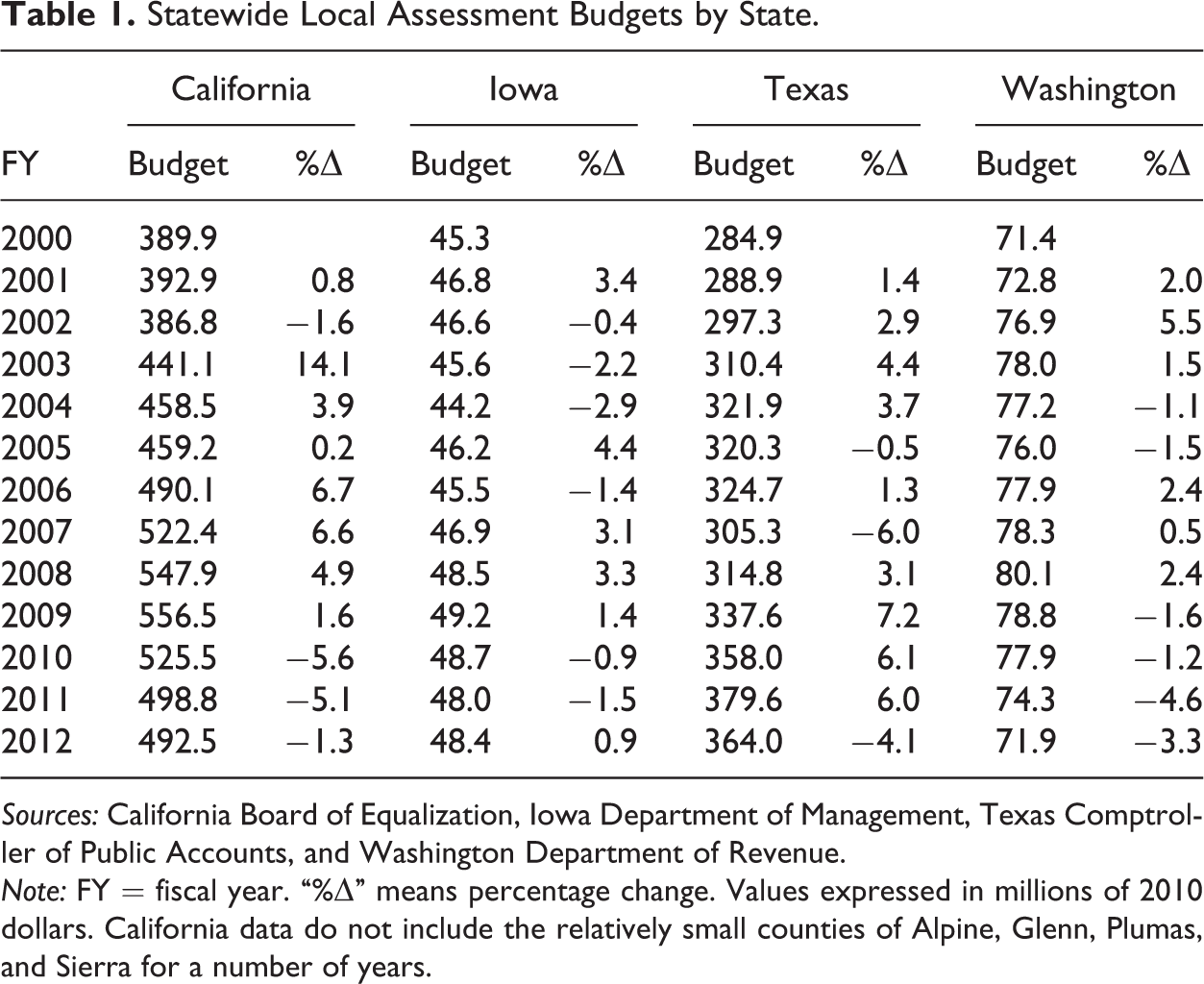
Sources: California Board of Equalization, Iowa Department of Management, Texas Comptroller of Public Accounts, and Washington Department of Revenue.

Note: FY = fiscal year. “%▵” means percentage change. Values expressed in millions of 2010 dollars. California data do not include the relatively small counties of Alpine, Glenn, Plumas, and Sierra for a number of years.

A number of empirical studies have explored the impact of changing housing market conditions on assessment outcomes. Bowman and Mikesell (1978, 1989) and Bowman and Butcher (1986) found that median home values are positively associated with COD levels in Virginia. Chicoine and Giertz (1988) found the same relationship in Illinois. In at least two cases, though, the association was not borne out. Kim (1987) found a null relationship in Georgia, and Eom (2008) discovered that home values and residential CODs were negatively related in New York.

One explanation for the inconsistencies is the nature of the housing data being used, namely, Census data.³ Administrative responses to short-term and long-term fluctuations in home prices cannot be distinguished from each other using data spanning ten years. Figure 1 illustrates this criticism by comparing the annual change in the Case-Shiller home price index to the decennial change from 1959 through 2012. Based on Census data (dotted line), the market expansion and contraction between 2001 and 2009 is not obvious. Indeed, one could view this period as a time of slow growth, rather than rapid growth and decline, because the overall ten-year change is positive. As a result, Census data provide policy makers and assessors little guidance for creating policies that help maintain high levels of assessment performance during periods of price volatility.

Figure 1.

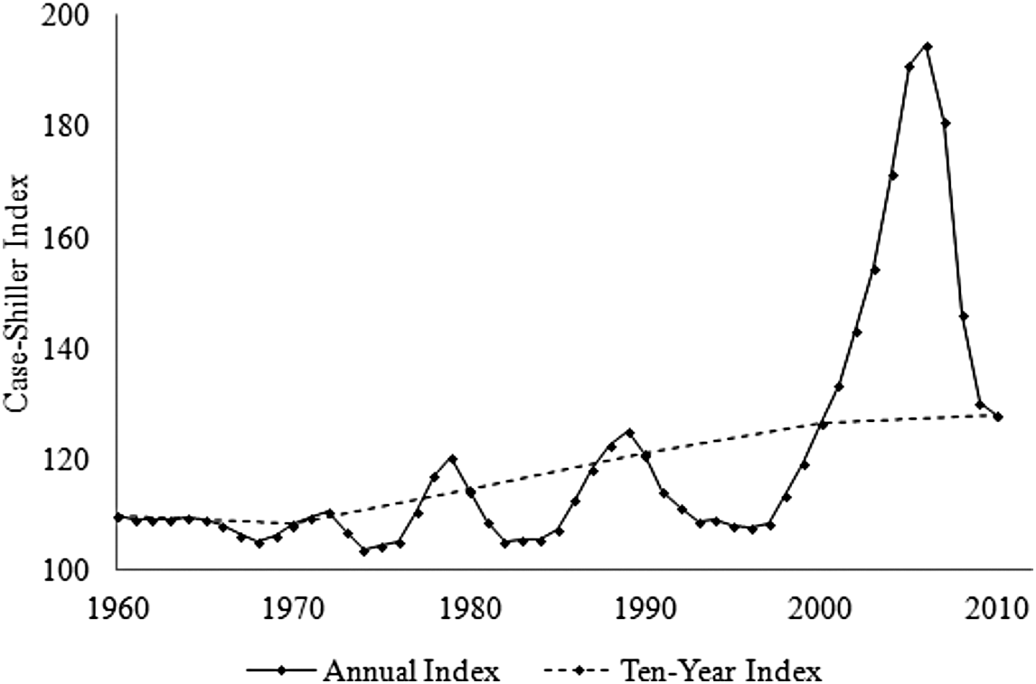
Case-Shiller index, 1960–2010.

Rapid changes in home prices indirectly affect the cost of assessments, and therefore they represent negative productivity (supply) shocks exogenous to the assessment process. Productivity shocks affect the amount of output that can be produced for a given amount of inputs by temporarily shifting the short-run supply curve inward or outward depending on the direction of the shock. In the short run, negative housing price shocks reduce assessor resources and increase appraisers’ task complexity thereby leading to a decrease in assessment output. When output is measured by the COD, the result is a decline in assessment uniformity, or alternatively an increase in assessment dispersion. Resource shocks can also impact assessor’s long-run productivity by permanently shifting the supply curve. The introduction of computer-assisted mass appraisal is an example of a positive productivity shock with permanent effects on assessment output.

Policy responses to short-lived assessment productivity shocks differ significantly from long-lived changes. For example, if over ten years a trend emerges associating increasing home prices with declining assessment equity, the appropriate policy response to improve equity, as Bowman and Mikesell (1978) and Bowman and Butcher (1986) argued, is to introduce more generous property tax relief through the assessment system. If steep home price fluctuations are transitory, however, the appropriate policy response is not to permanently erode the tax base through assessment relief but instead to increase assessor resources or to temporarily suspend or extend relief, depending on the type of properties experiencing price volatility. The amount of additional resources depends on the shock’s magnitude while the magnitude and duration of relief depends on the shock’s impact on assessment error.

In order to clarify the relationship between rapidly changing home prices and assessment performance, residential CODs are regressed against administrative and environmental factors previous research has identified as crucial to assessment outcomes. Two unique variables indicating housing price shocks are also included. The model and variables used for the analysis are detailed next.

Empirical Model and Variables

The output of a market-based assessment system is determined by the production function: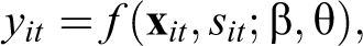

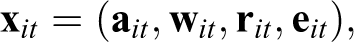
y_{i t} = f (x_{i t}, s_{i t}; β, θ),

where y_it is the level of output in county i in year t, x is a vector of inputs, s_it is a variable indicating the presence of a housing shock, and β and θ are parameters to be estimated. The assessment administration literature has identified various inputs the influence output levels. Accordingly,

x_{i t} = (a_{i t}, w_{i t}, r_{i t}, e_{i t}),

where a is a vector of characteristics of each county’s assessment system, measured by physical inspection frequency and level of assessment; w is a vector of each county’s assessment workload, measured by the number of residential parcels per real property appraiser and the percentage of a county’s total parcel count with new construction; r is a vector of each county’s assessment resources, measured as assessors’ budget per residential parcel and concentration of appraisers; and e is a vector of environmental characteristics that influence assessment output, measured as per capita income and unemployment. The production function is assumed to be logarithmic, and the equation to be estimated is

l n y_{i t} = α_{i t} + θ s_{i t} + Σ β_{k} l n x_{i t} + ε_{i t},

where α is a constant and ∊ is a disturbance term. Following the selection criteria advocated by Griffin, Montgomery, and Rister (1987), the logarithmic form is the appropriate strategy for a number of reasons. The form’s flexibility is desirable because it does not impose restrictions on output levels when any input equals zero. Because of how housing shocks are coded, which is discussed in the next section, allowing output to vary when inputs take zero values is a desirable property. The logarithmic form also has the advantage of being able to more easily incorporate a large number of inputs, as compared to generalized Cobb–Douglas or translog forms, for instance. A third reason is that the data for the independent variables were positively skewed. Converting them to logarithms thus makes them more normally distributed.

Dependent Variable

The dependent variable is expressed as the natural log of the COD for residential properties where “residential” is defined as single-family and multifamily properties.⁴ The COD measures variability in property assessments relative to the median level of assessment. It is calculated as the average difference between a given assessment ratio and the median ratio divided by the median multiplied by 100. A COD of zero percent indicates no dispersion around the mean—that is to say that all properties were assessed identically. Lower CODs therefore imply greater horizontal assessment equity. Said differently, a positive coefficient indicates that a variable negatively impacts assessment equity because it increases dispersion.

As discussed by Geraci (1977) and Bowman and Mikesell (1978), the natural log of the COD is used for two reasons. First, it is more normally distributed than the nonlogged form. Second, the arithmetic COD assumes assessment output levels vary proportionately with input levels, which is counterintuitive. A 50 percent improvement in the COD from 20 percent to 10 percent will require fewer resources (i.e., costless) than what would be needed to improve the COD from 5 percent to 2.5 percent. The nonlinearity of output level with respect to assessment costs was confirmed empirically by Sjoquist and Walker (1999) using data from Georgia.

Independent Variables

There are five groups of variables corresponding to the factors predicted to impact COD output: housing market shocks, features of the assessment system, assessor workload, assessor resources, and environmental factors. Each is discussed in turn.

Housing Market Shocks

Housing market shocks are measured in two ways. First, a dummy variable is used to identify a market contraction. The variable equals one when the annual percentage change in a county’s real median home price is negative and zero otherwise. A positive coefficient would indicate that housing market contractions are associated with greater levels of dispersion. Second, a trend variable is used to estimate the marginal impact of median home price declines. The variable takes a value between zero and fifteen. When the annual percentage change in real median home prices is greater than or equal to zero, the variable takes a value of zero. It takes a value of one when the annual change is less than zero and greater than or equal to negative one, a value of two when the annual change is less than negative one and greater than or equal to negative two, and so forth until fifteen, which denotes an annual negative change greater than 14 percent. Because rapidly changing market conditions inhibit otherwise high-quality assessments (Engle 1975; Borland 1990), the coefficients for the housing shock variables are predicted to be positive—that is, contractions are expected to increase dispersion.

Assessment System

Two variables capture features of each county’s assessment system: its physical inspection cycle and level of assessment. With respect to the first, frequent inspections help appraisers easily identify property features that affect market value. The more often properties are inspected the more likely properties will be assessed closer to their market value. Washington state law requires counties to physically inspect property at least once every six years.⁵ In 2011, twenty-three counties required inspections every sixth year. Previous research shows that more frequent revaluations improve assessment uniformity (Bowman and Butcher 1986; Lloréns-Rivera 1996; Mikesell 1980). By extension, then, more frequent physical inspections are expected to reduce assessment dispersion. It is noteworthy that in at least one study, though, no statistically significant relationship between inspection frequency and level of uniformity was found (Strauss and Sullivan 1998).

Counties’ assessment levels are reflected in ASRs, which measure the assessed value of a property relative to its sales price. Whereas CODs measure assessment precision, ASRs measure assessment accuracy. Intuitively, the relationship between ASRs and CODs is negative: as the median ASR approaches one, the COD approaches zero. A considered explanation for the relationship suggests that as ASRs approach one, taxpayers gain better information about their property’s market value, which is then used in an assessment appeals decision calculus that ultimately improves assessment equity (Bowman and Mikesell 1978). The negative relationship between ASRs and uniformity has been consistently demonstrated in empirical work in other states (Bowman and Mikesell 1978, 1989; Bowman and Butcher 1986; Kim 1987; Lloréns-Rivera 1996). Thus, a negative relationship is also expected in Washington counties.

Assessor Workload

Workloads directly impact assessment quality by reducing the amount of time and effort appraisers are able to expend on each property account. To capture the effect of workload, two variables are used. The first variable is the number of residential parcels per real property appraiser. Because some county assessors employ part-time appraisers, Washington’s Department of Revenue (DOR) measures appraisers on staff in terms of full-time equivalency. In 2011, per parcel workloads ranged from 2,706 in Columbia County to 16,869 in Lincoln County. The expected sign of the coefficient is not clear. While smaller workloads have been argued to improve assessment performance (California Legislative Analyst’s Office 1997), the only empirical study exploring this dimension of assessment administration found that higher workloads reduced dispersion (Kim 1987). Despite the coefficient’s statistical significance, the author rejected the finding as inconsistent with any hypothesis.

One explanation for Kim’s finding is roll copying or the act of copying roll values from one year to the next (Mikesell 1980). As workload increases, appraisers have a greater incentive to rollover assessed values for existing housing stock in order to put more attention into new parcels that have not yet been assessed. To account for this possibility, a second workload variable measuring the size of base expansions is included. More precisely, the variable is the percentage of real parcels in each county with new construction.⁶ If the roll copying hypothesis has merit, the coefficients for the workload variables will have opposing signs. That is, because newer parcels are assessed closer to market value, as the concentration of parcels with new construction in a county increases, dispersion levels decrease.

Assessor Resources

In the course of their duties, appraisers collect a substantial amount of property data, and the assessment system’s ability to efficiently and effectively use these data to produce high-quality assessments depends on having adequate budgetary and personnel resources (Bird 2004). Two variables measure assessor resources: assessors’ budget per residential parcel and the concentration of appraisers on staff. The first variable reflects budgetary resources in proportion to each county’s taxable residential property base. The expected sign of the coefficient is uncertain. Eom (2008) found that increases in budgetary resources reduced dispersion; Kim (1987) failed to find a significant relationship; and Lloréns-Rivera (1996) found a nonsignificant relationship with 1982 data and a significant and negative relationship with 1992 data.⁷

The second variable measures the concentration of appraisers on staff and is calculated as the number of full-time equivalent appraisers divided by the total number of full-time equivalent employees. Previous research has relied on an indicator variable to denote use of full-time appraisers (Geraci 1977; Bowman and Butcher 1986; Bowman and Mikesell 1978, 1989). However, this strategy fails to account for different combinations of labor inputs that affect assessment output. The direction of the relationship between appraiser concentration and assessment uniformity is indeterminate. On one hand, higher concentrations of appraisers on staff could improve assessment quality by creating an environment that allows appraisers to exchange information about market conditions and appraisal techniques (Wincott 2002). On the other hand, higher concentrations of appraisers outside of assessors’ offices have been shown to be partially responsible for the housing bubble (Downs and Guner 2012), which, as discussed previously, is predicted to negatively impact assessment quality.

Environmental Factors

Factors external to the assessment system influence assessment outcomes (Ross 2012, 2013). Two variables, per capita income and unemployment rate, capture variations in socioeconomic conditions that may not be reflected in changes in the housing market. Previous research has found that personal income level is negatively associated with assessment error (Haurin 1988). Because smaller assessment errors imply greater assessment uniformity, the expected relationship between income and dispersion is negative. Moreover, research has found that unemployment levels are positively related to the annual growth of residential properties’ assessed values (Makowsky and Sanders 2010). However, it is not clear how appraisers perform in relationship to actual selling prices. If selling prices grow faster than assessed values, assessment uniformity declines, all other thing constant; if they grow slower, uniformity increases. The expected relationship between unemployment levels and dispersion is thus indeterminate.

Data

Data were retrieved from a number of sources. CODs and ASRs were obtained from annual sales ratio reports. From 2006 to 2009, the state House Appropriations Committee staff published the reports; and from 2010 onward, the DOR began publishing them for internal use. Drawing the dependent variable from disparate sources raises concerns about the data’s reliability. DOR staff was contacted to clarify the sampling and reporting processes used for both reports. They confirmed that over the observation period all sampling was conducted by the DOR using the same set of sampling criteria and that only one report was published each year. The only difference between the two is that Appropriations Committee staff calculated CODs and ASRs in one case and DOR staff in the other. Due to omitted data in the Appropriations Committee reports, Garfield County was dropped from the panel. Since the county only accounted for 0.05 percent and 2.4 percent of the state’s overall residential parcel count and statewide residential tax base, respectively, at the peak of the housing bubble in 2006, the omission would not demonstrably affect the results.

Median housing price data used to construct the housing shock variables were obtained from the Washington Center for Real Estate Research. Prices were adjusted to the Seattle-Tacoma-Bremerton Consumer Price Index. Housing market data for three counties were incomplete over the observation period: two years were missing for Lincoln County and one year each for Klickitat County and Skamania County. These gaps were filled by backward calculation using the average change in property prices for each county as published by the DOR in their annual Property Tax Statistics reports. Data on physical inspection cycles, workload, and resources were obtained from the DOR’s annual Comparison of County Assessor Statistics reports. Area income and unemployment rate data were obtained from the Bureau of Economic Advisors and Bureau of Labor Statistics websites, respectively. Variable descriptions and sources are summarized in table 2, and descriptive statistics are detailed in table 3.

Table 2.

Variable Descriptions and Sources.

Variable	Description	Source
Residential COD	Coefficient of dispersion for residential housing	1, 2
Housing shock (dummy)	1 if annual change in median home prices was less than zero, 0 otherwise	3, 4
Housing shock (categorical)	1 if annual change in median home prices was less than 0 and greater than or equal to −1; 2 if less than −1 and greater than and equal to −2; and so forth, 0 if annual change was greater than or equal to zero	3, 4
Physical inspection cycle	1 if county requires physical inspection of taxable real property every five or six years, 0 otherwise	2
Residential median ASR	Median ratio of residential assessed value to sales price	1, 2
Residential parcels per appraiser	Number of residential parcels per full-time equivalent real property appraiser in thousands	2
Percentage of base with new construction	Percentage of real parcels with new construction	2
Assessor’s budget per residential parcel	Assessor’s total budget per residential parcel	2
Concentration of appraisers of staff	Number of full-time equivalent real property appraiser divided by number of full-time equivalent employees	2
Real per capita income	County per capita income in thousands of 2010 dollars	5
Unemployment rate	County unemployment rate	6

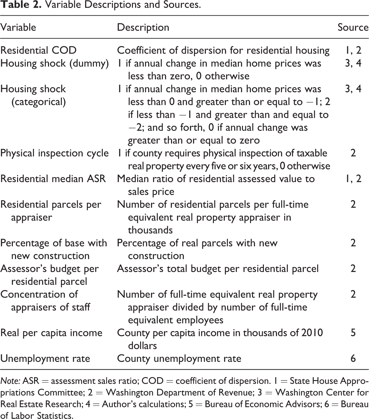
Note: ASR = assessment sales ratio; COD = coefficient of dispersion. 1 = State House Appropriations Committee; 2 = Washington Department of Revenue; 3 = Washington Center for Real Estate Research; 4 = Author’s calculations; 5 = Bureau of Economic Advisors; 6 = Bureau of Labor Statistics.

Table 3.

Descriptive Statistics.

Variable	M	SD	Min.	Max.
Residential COD	15.65	6.68	4.00	41.00
Housing shock (dummy)	0.62	0.49	0.00	1.00
Housing shock (categorical)	4.81	5.14	0.00	15.00
Physical inspection cycle	4.91	1.12	2.00	6.00
Residential median ASR	0.90	0.08	0.57	1.13
Residential parcels per appraiser (000s)	6.57	2.88	1.77	32.41
Percentage of base with new construction	3.11	1.92	0.36	10.22
Assessor’s budget per residential parcel	25.64	12.87	2.80	173.48
Concentration of appraisers of staff	0.49	0.10	0.20	1.00
Real per capita income (000s)	37.27	7.68	22.03	69.81
Unemployment rate	8.86	5.40	3.40	42.80

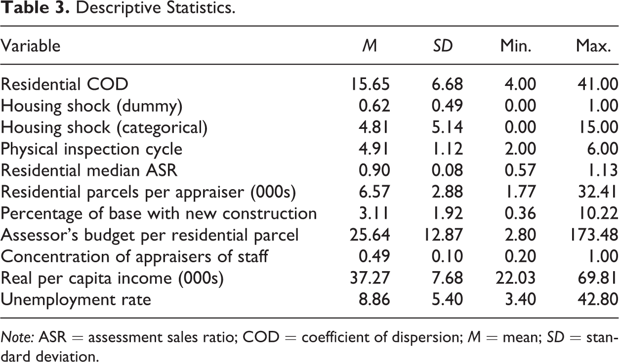
Note: ASR = assessment sales ratio; COD = coefficient of dispersion; M = mean; SD = standard deviation.

Washington is an ideal state to study because property is assessed at 100 percent of full market value, there are no assessment limitations, the state offers counties flexibility in establishing assessment practices such as frequency of physical inspections, and the DOR collects a large amount of data on county assessment practices each year.⁸ Unfortunately, Washington’s combination of circumstances also makes generalizability of this study to other states more challenging. In fact, only thirteen other states tax at 100 percent of full market value and do not have residential assessment limits, according to the most recent data in the Significant Features of the Property Tax database (Lincoln Institute of Land Policy 2013).⁹ Of these thirteen, only Alaska comes close to collecting the same level of data on local assessment practices as Washington. Thus, even if more states shared Washington’s institutional features, empirically verifying that the findings in this study are robust across states would remain difficult.

Empirical Results

A number of tests were used to identify the estimation strategy. A Wald test revealed the panel had a nonconstant variance and a Wooldridge test revealed serial correlation. Ordinary least squares was thus judged inappropriate. This conclusion was further supported by the Breusch–Pagan Lagrange multiplier test that rejected the null hypothesis of no panel effect. The tests also demonstrate that robust standard errors are required. Moreover, using the Schaffer-Stillman test, which unlike the more common Hausman is robust to heteroscedastic errors, the null hypothesis that the random effects coefficients are unbiased when the fixed effects coefficients are not was rejected. The regression results are displayed in table 4. Because housing shocks were measured in two different ways, separate regressions for each variable were run. Model 1 uses the housing shock dummy variable, and model 2 uses the categorical variable. In both models, the independent variables explain more variation between groups than within groups. The variables accounting for the assessment system, assessor resources, and assessor workload explain about 50 percent of the observed within-group variation.

Table 4.

Fixed-effects Regression Results.

Variable	Model 1	Model 2
Housing shock (dummy)	.080** (.033)
Housing shock (categorical)		.104** (.004)
Residential median ASR	−.732* (.402)	−.789* (.401)
Physical inspection cycle	−.416 (.273)	−.406 (.274)
Residential parcels per real appraiser	.283** (.119)	.289** (.124)
Percentage of base with new construction	−.134** (.050)	−.118** (.048)
Assessor’s budget per residential parcel	.197 (.118)	.186 (.123)
Concentration of real appraisers on staff	.207 (.222)	.221 (.226)
Real per capita income	−1.31** (.383)	−1.31** (.389)
Unemployment rate	−.046 (.438)	−.037 (.053)
Constant	4.58** (1.78)	4.62** (1.81)
N	228	228
R ² within	.199	.211
R ² between	.367	.364
R ² overall	.307	.309
Prob > F	.000	.000

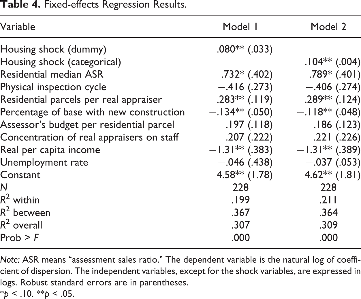
Note: ASR means “assessment sales ratio.” The dependent variable is the natural log of coefficient of dispersion. The independent variables, except for the shock variables, are expressed in logs. Robust standard errors are in parentheses.

*p < .10. **p < .05.

Consistent with expectations, both models report that housing market contractions are negatively related to residential assessment quality. From model 1, a housing market contraction increases dispersion by 8 percent, which is substantially larger than the magnitudes reported in the earlier studies using Census data. To gauge the sensitivity of the shock coefficient to assessor resources and workload, the variables in the two categories were omitted. The magnitude of the dummy housing shock coefficient increased to 0.10 (p < .05).

Model 2 shows the marginal effect of a declining housing market on COD levels. Each percentage decline in annual median home sales price increases residential dispersion by 11 percent, holding everything else constant. A county experiencing a housing contraction between 4 and 5 percent is therefore predicted to have a residential COD roughly six times greater than a county with a contraction between zero and 1 percent. The relationship between change in COD output and marginal declines in the housing market is illustrated in figure 2. The largest change in assessment performance occurs during the initial stages of a housing market contraction; from zero and 1 percent to 1 and 2 percent, residential dispersion increases 112 percent, holding the other variables constant. Moreover, uniformity worsens at a diminishing rate. This can be explained by the fact that larger market contractions affect a larger sample of homes. Larger contractions therefore produce greater clustering around the median ASR even as the median ASR declines. Taken together, the two shock coefficients not only demonstrate that the Great Recession had a substantial negative impact on assessment performance in Washington counties but also that the greatest decline in horizontal assessment equity occurs in the early stages of a housing market contraction.

Figure 2.

Percentage change in residential coefficient of dispersion by housing market contraction size.

The direction of the ASR coefficients is consistent with expectations and previous research: higher levels of assessment are associated with greater assessment equity. Specifically, a 1 percent increase in the ASR in Washington counties over the observation period is associated with a 0.73 to 0.79 percent decrease in assessment dispersion. The magnitude of the relationship is twice as large as Kim’s (1987) finding, which is based on 1984 data. This suggests that improvements in assessment administration over the last three decades have greatly increased the horizontal equity return from greater investments in technology and professionalization. Coupled with the shock coefficients, the results of the two models suggest that some homeowners received de facto assessment relief due to poorer appraisal job performance during the Great Recession. That is, as the median ASR is pulled downward due to increasing job complexity, holding all other observables fixed, assessment uniformity declines.

More frequent physical inspections were expected to improve assessment equity, yet the coefficient for the inspection variable is not statistically significant (p < .137), a finding consistent with Strauss and Sullivan (1998). This could reflect the uniqueness of the observation period. During bubbles when properties turnover at higher rates, improvements between sales will be capitalized into observable market prices. During market contractions, property owners may be less willing to invest in improvements that increase their property’s value. In both instances, inspections between sales are less likely to reveal assessable improvements and thus are less likely to influence assessment dispersion. Alternatively, as states increase the types of improvements that are excluded from assessment, the impact of more frequent inspections on ASRs declines.

The assessor workload variables were predicted to have opposing influences on residential COD, and indeed this is observed. From models 1 and 2, a 10 percent increase in the number of residential parcels per appraiser results in a 2.8 percent increase in residential dispersion. This result is consistent with the assertion that smaller workloads improve assessment outcomes. In addition, it was hypothesized that higher concentrations of new property would improve assessment equity by reducing the opportunity to roll copy, and the relevant coefficient has the predicted sign: a 10 percent increase in the concentration of parcels with new construction reduces assessment dispersion by slightly more than 1 percent. While the results do not directly indicate that roll copying is prevalent in practice, it does lend support to the theory that roll copying declines in rapidly expanding housing markets.

The predicted signs for the assessor resource coefficients were indeterminate. With respect to assessors’ budgets per residential parcel, the coefficient is not statistically significant, which is consistent with Kim (1987). A possible explanation for why assessors’ budgets do not appear to improve residential uniformity is that there are economies of scale in assessment production (Mehta and Giertz 1996; Sjoquist and Walker 1999). The annual variation in assessors’ budgets over the observation period thus may not be substantial enough to influence output levels. This reasoning implies that in the short run cutting budgets improves the economic efficiency of property assessments. With respect to the concentration of appraisers, the coefficient is also not significant. While the null result does not indicate that more appraisers will not improve assessment equity, it also does not support the hypothesis that investing in more appraisers creates a better marketplace of ideas (Wincott 2002).

Environmental factors external to the assessment process were found to have mixed influence on residential COD. Consistent with Haurin (1988), area personal income levels are negatively associated with residential assessment dispersion. The magnitude of the relationship is also the largest of the variables in the two models. The expected sign for unemployment was indeterminate and the coefficient in both models is not statistically significant.

Model 1 establishes that assessment uniformity declined when Washington’s housing market contracted, and model 2 demonstrates that assessment uniformity declined at a declining rate. Neither model indicates whether the effects of housing price shocks on uniformity are short-lived or long-lived, however, which is important to know because the appropriate policy response depends on the expected life of the problem. While the diminishing rate of growth in residential dispersion suggests the negative impact of market contractions on assessment performance is transitory, a more decisive conclusion can be reached by allowing the influence of housing shocks to vary over time. Interaction terms defined as the multiplicative of the categorical shock variable for each year were created (2006 is the reference group). The test for a transitory or permanent effect lies in the statistical significance of the interaction coefficients and their magnitude over the observation period. The hypothesis that the Great Recession had long-lived negative impacts on assessment equity is supported if all interaction coefficients are significant and their magnitudes are relatively similar. If the impact is transitory, interaction terms will be significant in early years and not significant in later years, and further the magnitudes will decline over time. The interaction coefficients indicate transitory impacts: after 2009, the interaction coefficients lose statistical significance. (Specifically, for the 2008 interaction term, β = −.034, p < .05, and for the 2009 interaction term, β = −.028, p < .10.) Said differently, within two years of the housing market’s collapse, the Great Recession’s impact cannot be statistically distinguished from other sources of random assessment error.

Policy Implications

Local government revenue was a casualty of the Great Recession. With attention focused on raising revenue, however, assessment performance suffers. In theory, assessment performance is expected to decline in recessionary economies, first, because of increased task complexity due to rapidly changing environmental conditions, and, second, because of budget cuts that reduce assessors’ resources. While the results in this study indicate that falling home prices do indeed reduce assessment quality, the effects of price shocks are short-lived and are not statistically influenced by annual variations in assessors’ resources.

The null effect of assessors’ budgetary resources begs the question, if additional resources do not improve assessment equity in declining markets, what other policy alternatives exist to maintain high levels of performance? A number of alternatives are at assessors’ and policy makers’ disposal. For example, assessors could reallocate existing resources in anticipation of market contractions. As previously noted, the lack of significance of budgets on residential COD suggests the average assessor was not operating at economically efficient levels. By shifting excess resources away from overly consumed factor inputs to appraisal labor, which this study showed reduces dispersion, assessors could offset declines in performance during periods of market contractions. Since the observed impact is transitory, resource reallocations would only need to be temporary, and the steps taken to reduce appraiser workload would be most beneficial in the early stages of falling home prices when the negative influence on uniformity is the greatest. This option could perhaps be most easily implemented by creating rainy day funds to help assessors smooth expenditures over time.

A second policy alternative is to increase the frequency of physical inspections. In order to minimize variations in the level of assessments, and therefore variations in COD, properties with the largest swings in prices should be targeted for inspection. Recently compiled data show that lower-priced homes had steeper price declines than did higher-priced homes, and the relationship was robust across US metropolitan areas (Cohen, Coughlin, and Lopez 2012). Because of the amount of work involved in more frequent inspections, however, existing resources would certainly be insufficient. Additional budgetary allocations would thus be required.

In addition, it was previously noted that some Washington property owners received de facto assessment relief due to poorer appraisal job performance during the Great Recession. Depending on the types of properties affected, the combination of de facto and statutory relief could exacerbate assessment inequities rather than ameliorate them. In the face of rapidly contracting prices, the combination of de facto and statutory relief could drag down the median ASR beyond a desirable level. As a result, because of the negative relationship between median ASR and COD, assessment dispersion would increase. An appropriate policy response for maintaining assessment equity in declining markets then is to temporarily suspend or lower the statutory relief for those properties enjoying de facto relief.

However, this policy response is only appropriate if the homes receiving statutory relief are the same homes receiving de facto relief—that is, the homes eligible for statutory relief are the same homes that are more complicated to accurately assess because of rapidly changing market conditions. While the present study does not directly address this matter, Cohen, Coughlin, and Lopez’s (2012) data suggest that lower-priced properties were more difficult to assess during the Great Recession because they had higher swings in value. Since most assessment relief programs target lower-priced residences, it stands to reason that such properties received the de facto relief while higher-priced properties with smaller swings in value did not. By extension, if lower-priced homes were in fact the benefactors of de facto relief, the appropriate policy response for arresting declines in median ASR would be to temporarily suspend or lower statutory relief for lower-priced homes or to temporarily extend statutory relief to higher-priced homes. The latter may be more politically feasible on the logic that homeowners of lower-priced homes should not be penalized for assessment errors. The consequences of granting relief to higher-priced properties, however, is a smaller base and, to the extent the relief is greater than the de facto relief given to lower-priced properties, a shifting of tax liabilities from homeowners most able to pay to those least able to pay. It is left to future research to determine if lower-priced homes are in fact the benefactors of de facto relief in contracting markets.

Conclusion

This study explored the performance of assessment administration during the Great Recession using data from Washington state counties. The housing bust was treated as a productivity shock to the assessment process. Due to rapidly changing environmental conditions and declining assessor resources, assessment performance, as measured by the residential COD, was predicted to suffer. Only the former condition was found to impact residential assessment uniformity, however. Furthermore, the increased task complexity in an environment of falling home prices suggests that homeowners experiencing wide swings in market value received de facto assessment relief.

The conclusions reached in this study should be accepted tentatively for two reasons. First, the analysis only focuses on one state and therefore may not be generalizable to other jurisdictions. Second, the analysis did not control for individual-level appraiser characteristics. The study accounted only for the concentration of appraisers on staff rather than their age, experience, or education. However, the relative effect of these characteristics on assessment performance during periods of rapidly declining home prices is far from clear. The magnitude of the housing bust may have neutralized any performance advantages more experienced appraisers might have had over less experienced appraisers.

This study has also exposed a number of avenues for future research. One line of fruitful inquiry would be to explore the relationship between property tax base erosion and assessment outcomes. It was suggested that as the number of improvements excluded from assessment increases, equity suffers. These types of improvements include the addition of alternative energy systems such as solar panels or renovations for disabled persons. A second line of research could involve a more thorough exploration of the relationship between the volume of lower-priced homes sold and assessment outcomes. The conclusion that lower-priced homes drive assessment inequities in contracting housing markets is only speculative, and the suggested policy response of temporarily curbing their statutory relief should not be considered until a more thorough investigation has been conducted. Finally, the null effect of budgetary resources on assessment uniformity deserves further study. Other states should be investigated to see whether the nonrelationship is robust.

Footnotes

Authors’ Note

The author is solely responsible for all errors.

Acknowledgments

The author is indebted to editor James Alm, David Brunori, Catherine Collins, Joseph Cordes, and two anonymous referees whose constructive criticisms significantly improved the quality of this study.

Declaration of Conflicting Interests

The author(s) declared no potential conflicts of interest with respect to the research, authorship, and/or publication of this article.

Funding

The author(s) received no financial support for the research, authorship, and/or publication of this article.

Notes

References

Aaron

Henry J.

1977. “Commentary: Nonparametric Statistics and the Measurement of Assessment Performance.” In Analyzing Assessment Equity, 103–6. Chicago: International Association of Assessing Officers.

Alm

James

Buschman

Robert D.

Sjoquist

David L.

. 2011. “Rethinking Local Government Reliance on the Property Tax.” Regional Science and Urban Economics 41:320–31.

Anderson

John E.

2010. “Shock to the Property Tax Base and Implications for Local Public Finance.” Paper presented at the Housing Crisis and Its Effects on State and Local Government Conference, Washington, DC, May 20–21.

Benson

Earl D.

Schwartz

Arthur L.

. 1997. “Vertical Equity in the Taxation of Single-family Homes.” Journal of Real Estate Research 14:215–31.

Bird

Richard M.

2004. “Administrative Dimensions of Tax Reform.” Asia-Pacific Tax Bulletin 10:134–50.

Borland

Melvin V.

1990. “On the Degree of Property Tax Assessment Inequity in Complex Tax Jurisdictions.” American Journal of Economics and Sociology 49:431–38.

Bowman

John H.

Butcher

William A.

. 1986. “Institutional Remedies and the Uniform Assessment of Property: An Update and Extension.” National Tax Journal 39:157–69.

Bowman

John H.

Mikesell

John L.

. 1978. “Uniform Assessment of Property: Returns from Institutional Remedies.” National Tax Journal 31:137–52.

Bowman

John H.

Mikesell

John L.

. 1989. “Elected versus Appointed Assessors and the Achievement of Assessment Uniformity.” National Tax Journal 42:181–89.

10.

California Legislative Analyst’s Office. 1997. Improving the Incentives for Property Tax Administration. Sacramento: California Legislative Analyst’s Office.

11.

Chernick

Howard

Langley

Adam

Reschovsky

Andrew

. 2011. “The Impact of the Great Recession and the Housing Crisis on the Financing of America’s Largest Cities.” Regional Science and Urban Economics 41:372–81.

12.

Chicoine

David L.

Giertz

J. Fred

. 1988. “Uniformity in a Dual Assessment System.” National Tax Journal 41:247–56.

13.

Cohen

Jeffrey P.

Coughlin

Cletus C.

Lopez

David A.

. 2012. “The Boom and Bust of US Housing Prices from Various Geographic Perspectives.” Federal Reserve Bank of St. Louis Review 94:341–67.

14.

Conant

James K.

2010. “Introduction: The “Great Recession,” State Budgets, and State Budget Deficits.” Public Budgeting & Finance 30:1–14.

15.

Downs

David H.

Z. Nuray

Guner,

. 2012. “Information Producers and Valuation: Evidence from Real Estate Markets.” The Journal of Real Estate Finance and Economics 44:167–83.

16.

Egan

Marcia

Kadushin

Goldie

. 2004. “Job Satisfaction of Home Health Social Workers in the Environment of Cost Containment.” Health & Social Work 29:287–96.

17.

Engle

Robert F.

1975. “De Facto Discrimination in Residential Assessments: Boston.” National Tax Journal 28:445–552.

18.

Eom

Tae Ho

. 2008. “A Comprehensive Model of Determinants of Property Tax Assessment Quality: Evidence in New York State.” Public Budgeting & Finance 28:58–81.

19.

Geraci

Vincent J.

1977. “Measuring the Benefits from Property Tax Assessment Reform.” National Tax Journal 30:195–205.

20.

Griffin

Ronald C.

Montgomery

John M.

Rister

M. Edward

. 1987. “Selecting Functional Form in Production Function Analysis.” Western Journal of Agricultural Economics 12:216–27.

21.

Groves

Harold M.

Goodman

A. Bristol

. 1943. “A Pattern of Successful Property Tax Administration: The Wisconsin Experience-III. Local Assessment and Its Results.” The Journal of Land & Public Utility Economics 19:418–35.

22.

Haurin

D. R.

. 1988. “An Empirical Analysis of Property Tax Equity.” Property Tax Journal 7:5–18.

23.

Hillhouse

Joel J.

Adler

Christine M.

. 1997. “Investigating Stress Effect Patterns in Hospital Staff Nurses: Results of a Cluster Analysis.” Social Science & Medicine 45:1781–88.

24.

Kim

Jong-Soon

. 1987. “Property Tax Assessment Administration in Georgia: The Determinants of Assessment Accuracy.” Unpublished PhD diss. The University of Georgia, Athens.

25.

Levine

Helisse

Scorsone

Eric

. 2011. “The Great Recession’s Institutional Change in the Public Employment Relationship Implications for State and Local Governments.” State and Local Government Review 43:208–14.

26.

Lincoln Institute of Land Policy. 2013. “Significant Features of the Property Tax: Tax Limits and Value Standard and Assessment Ratios.” Accessed March 2, 2013. http://www.lincolninst.edu/subcenters/significant-features-property-tax/Topics.aspx.

27.

Lloréns-Rivera

Antonio

. 1996. “Factors Contributing to an Accurate Property Value Assessment System in the United States of America, 1982-1992.” Unpublished PhD diss. Ohio State University, Columbus.

28.

Lutz

Byron F.

Molloy

Raven

Shan

Hui

. 2011. “The Housing Crisis and State and Local Government Tax Revenue: Five Channels.” Regional Science and Urban Economics 41:306–19.

29.

Makowsky

Michael D.

Sanders

Shane

. 2010. “Political Costs and Fiscal Benefits: The Political Economy of Residential Property Value Assessment.” Working Paper No. 2010-16, Department of Economics, Towson University, Towson, MD.

30.

Mehta

Shekhar

Giertz

Fred

. 1996. “Measuring the Performance of the Property Tax Assessment Process.” National Tax Journal 49:73–85.

31.

Mikesell

John L.

1980. “Property Tax Reassessment Cycles: Significance for Uniformity and Effective Rates.” Public Finance Quarterly 8:23–37.

32.

Ross

Justin

. 2012. “Interjurisdictional Determinants of Property Assessment Regressivity.” Land Economics 88:28–42.

33.

Ross

Justin

. 2013. “A Socioeconomic Analysis of Property Assessment Uniformity: Empirical Evidence on the Role of Policy.” Public Budget & Finance 33:49–75.

34.

Shiller

Robert

. 2012. “Historical Housing Market Data.” Accessed February 15, 2013. http://www.econ.yale.edu/∼shiller/data.htm.

35.

Sjoquist

David L.

Walker

Mary Beth

. 1999. “Economies of Scale in Property Tax Assessment.” National Tax Journal 52:207–20.

36.

Strauss

Robert P.

Sullivan

Sean R.

. 1998. “The Political Economy of the Property Tax: Assessor Authority and Assessment Uniformity.” State Tax Notes 15:1603–10.

37.

Wincott

Richard D.

2002. “A Primer on Comparable Sale Confirmation.” The Appraisal Journal 70:274–82.