



Abstract
This article assesses the fiscal implications of the 2012 Greek excise tax reform that involved the adoption of a common tax rate between automotive and heating diesel markets. Based on univariate and system estimation methods on demand models that account for linkages between energy markets, evidence of an elastic heating diesel demand is compared to automotive diesel demand with regard to excise taxation. Limited support of an immediate antiarbitrage effect is found in these diesel markets after the common rate adoption. This is attributed to the significant heating diesel stock accumulation and the longer horizon of relevant tax administration reforms. Ceteris paribus, the budgetary outcome of the 2012 reform is positive during its first year of implementation, evidenced by the higher rate introduced compared to the breakeven rate of €230/1,000 liters simulated in this analysis. Nevertheless, factors like income, weather conditions, and continuing arbitrage influence this outcome negatively.
Following a protracted period of external and fiscal imbalances, the 2010 Greek economic adjustment program involved a mix of significant expenditure cuts and revenue increases. The regular public debate on the program focused firstly on the growth repercussions of the fiscal consolidation that followed. Secondly, the debate focused on the program’s ineffectiveness to restrict the informal economy and the subsequent tax evasion.
The liquid fuel market, and particularly the diesel market, represents a good example of a market in Greece in which arbitrage is usually present. In an attempt to limit arbitrage between heating diesel and automotive 1 diesel through price convergence, the Ministry of Finance (MoF), in its 2012 excise taxation reform, adopted a single excise tax rate for both markets.
From a global perspective, governments tax energy fuels to raise revenues and fund highway infrastructure and services. Given the inelastic tax base, this source of public revenues is considered stable when combined with the low cost of collecting revenues.
Following the work of the Organization for Economic Cooperation and Development (2013) and Harding (2014), energy fuel taxation varies considerably between countries. These taxation differences express alternative national priorities for competitiveness, industrial policy, social policies, and so on. In addition, these differences apply to alternative energy fuels with the same use (e.g., diesel, gas, bioethanol used for transportation lately, etc.) and to different uses of the same fuel (transportation, heating, production, etc.). According to the US Association of Convenience and Fuel Retailing (NACS), (2013) 2 and Harding (2014) argue that these excise tax rate differences usually explain a notable part of the observed retail price differences in the case of the gasoline and automotive diesel markets.
According to the US National Center for Environmental Economics (2001), the most notable tax rate differences exist in the case of leaded and unleaded gasoline (higher tax rate on leaded gasoline), which reflect differences in their environmental impact. The same differences also exist in countries that, for the sake of environmental protection, tax leaded gasoline more than unleaded gasoline, for example, Australia, Mexico, New Zealand, Singapore, and most European countries.
The intention behind taxation changes in energy markets may be to increase public revenues and improve economic incentives. Nevertheless, adopting a common excise tax rate between different fuel uses may also be grounded on the policy objective to internalize adverse social costs (loss of public revenues) related to smuggling and arbitrage between these fuel markets. The Greek MoF 3 used this line of argument when stating that the option of a differential tax rate between heating and automotive diesel markets “would open up the door to diesel market smugglers.”
Moreover, national energy taxation plans are also subject to the European Commission (EC) directive (2003/96/EC), which sets minimum taxation limits that apply to different energy sources. Member states are allowed to differentiate between the commercial and the noncommercial use of diesel used as propellant (including commercial shipping), provided that the EC minimum levels are respected.
Being a member of the European Monetary Union, Greece has been among the member states applying a differential excise taxation rate during the winter period (i.e., 15 October to 30 April). For heating diesel, it was initially set at €21 per 1,000 liters. During the rest of the year, the usual automotive diesel excise tax rate (€420 per 1,000 liters) applied to heating diesel as well (figure 1).
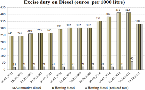
Diesel excise taxation.
Such a differentiated excise taxation scheme gave incentives for arbitrage and heating diesel quantities were used for consumption to the more heavily taxed automotive diesel market. After May 2010, the observed arbitrage profit was marginally reduced, since the heating diesel excise tax rate increased from €21 to €60 (per 1,000 liters). Finally in October 2012, the adoption of a common excise rate equal to €330 (per 1,000 liters) for both diesel markets throughout the year was introduced.
At the same time, to reimburse low-income families for the increase in heating diesel taxation, a heating benefit was introduced conditional to a set of criteria (i.e., the income of married couple less than €25,000 plus €3,000 additional income per child and the value of real-estate ownership less than €200,000 for married couples). Moreover, a set of maximum thresholds of heating diesel consumption per square footage was included in this reimbursement scheme based on the geographic location 4 of the residence. According to estimates, 5 the average amount reimbursed for the case of heating diesel was €0.25 per liters.
The purpose of this article is to examine the factors that determine diesel demand for automotive and heating purposes in Greece. Based on these empirical findings, the implications of the end-2012 excise tax reform are explored in terms of limiting existing arbitrage and increasing excise tax revenues.
The main conclusions of this article point, firstly, to a limited immediate arbitrage effect between the Greek diesel markets, and secondly, to the positive budgetary effect right after the adoption of the 2012 common excise tax rate. The common tax rate set in the 2012 excise tax reform is higher than the breakeven excise tax rate simulated in this analysis, which supports a positive budgetary outcome. However, this outcome is also influenced by various factors such as weather conditions, income effects, and continuing arbitrage that during 2013 limited the tax base and the relevant revenue collections.
This article contributes to the existing literature in a number of ways: Firstly, the analysis refers to a market (i.e., heating diesel) that, to the best of our knowledge, has not been explored before at an international level. This is made possible through using unpublished administrative data on diesel consumption. Secondly, a novel assessment is applied to capture the effect that excise tax equalization may have on arbitrage between substitute energy markets that provide an almost homogeneous product. Thirdly, the analysis also explores the budgetary implications of this equalization, which is a novelty in this area of research. Lastly, by assessing the Greek diesel markets with the most recent data, this is the only study that captures the recent crisis and the subsequent significant changes in consumption patterns and wealth. In this context, the existing relevant empirical literature on price and income elasticities in the diesel market reflects the precrisis period and cannot be used to assess current public policies. This work attempts to cover these issues in the literature.
The remainder of the article is organized as follows. The second section briefly reviews the empirical literature. The third section describes the structure of diesel oil taxation and demand in Greece. The fourth and fifth sections present the basic empirical model and the data employed. The sixth section presents the results of the empirical model. The seventh section discusses the policy implications for arbitrage and the government budget of the 2012 excise tax reform. And the eight section concludes.
Literature Review
Road energy demand conditions and their determinants have been extensively examined in a number of empirical studies. In general, they are grouped into two categories based on their estimation methodology.
Firstly, stationarity and cointegration (Engle–Granger) techniques are used to estimate long- and short-run price and income elasticities in various economies using long data spans (e.g., Dahl and Sterner 1991; Dahl 1986; Samimi 1995; Ramanathan 1999; Alves and Bueno 2003; Polemis 2006; Wadud, Daniel, and Noland 2009). Recently, Fotis and Polemis (2012) and Polemis and Fotis (2013, 2014) have also assessed price asymmetries and the reasons behind them in energy markets (i.e., for the euro area gasoline market).
Secondly, structural demand models are employed that capture determinants of road energy demand and estimate price and income elasticities. The articles of Baltagi and Griffin (1983), Dunkerley and Hoch (1987), and Ramanathan and Geetha (1998) apply this univariate equation demand specifications, providing estimates of income and price elasticities. Belhaj (2002) extends this approach to the neighboring gasoline markets in the United States and Canada, while Nicol (2003) uses this approach in supplementary markets (i.e., vehicle and fuel demand in Morocco). In all of these examples, a three stages least square (3SLS) system estimation is applied to avoid the simultaneity bias that the joint determination of price and quantity in market equilibrium causes.
Following the previous empirical literature, the Greek energy market has been previously examined in several studies, investigating various demand aspects of it (i.e., Donatos and Mergos 1989, 1991; Christodoulakis et al. 2000; Hondroyiannis, Lolos, and Papapetrou 2002; Hondroyiannis 2004; Rapanos and Polemis 2005, 2007). Despite the notable policy implications, only a limited number of studies investigate the demand conditions in the road liquid fuel markets in Greece (Polemis 2006) and their respective fiscal implications (Karavitis, Maniatis, and Danchev 2012).
Taxation Structures and Demand Interrelations in the Greek Diesel Market
Taxation on diesel in Greece provided for a differential rate between heating and automotive diesel during the heating period (figure 1), and a common rate reflecting the EC minimum rate (per 1,000 liters) during the remainder of the year. This tax differentiation led to an iceberg-type margin between 2002 and 2012, starting from €227 per 1,000 liters in 2002 to €352 per 1,000 liters before the common rate adoption. This margin increases between almost homogeneous products signaled the increase in the accompanying arbitrage.
Mardas (2012) in his survey of arbitrage practices in the Greek diesel market reports that arbitrage involves discoloring the heating diesel 6 for use as automotive diesel. 7 It is also common for smugglers to make “fake” exports of heating diesel to the neighboring Balkan countries. Heating diesel quantities are never actually exported and aim to cover indigenous automotive diesel demand after being mixed with the highly taxed automotive diesel. The retail selling of the adulterated diesel provides arbitrage profits close to the taxation differential weighted by the composition of the diesel mix.
Turning to the fiscal implications from the excise diesel taxation 8 (both heating and automotive), excise tax revenues from that source remained rather stable and close to €1.2 billion between 2010 and 2012. This source of revenue represents a significant part (almost 10 percent) of the total indirect consumption taxes. In view of the common tax rate adoption at the end of 2012 9 relevant annual MoF revenue forecasts, projected 10 at that time a rise of 13 percent in 2013 and of 14 percent in 2014 (figure 2).
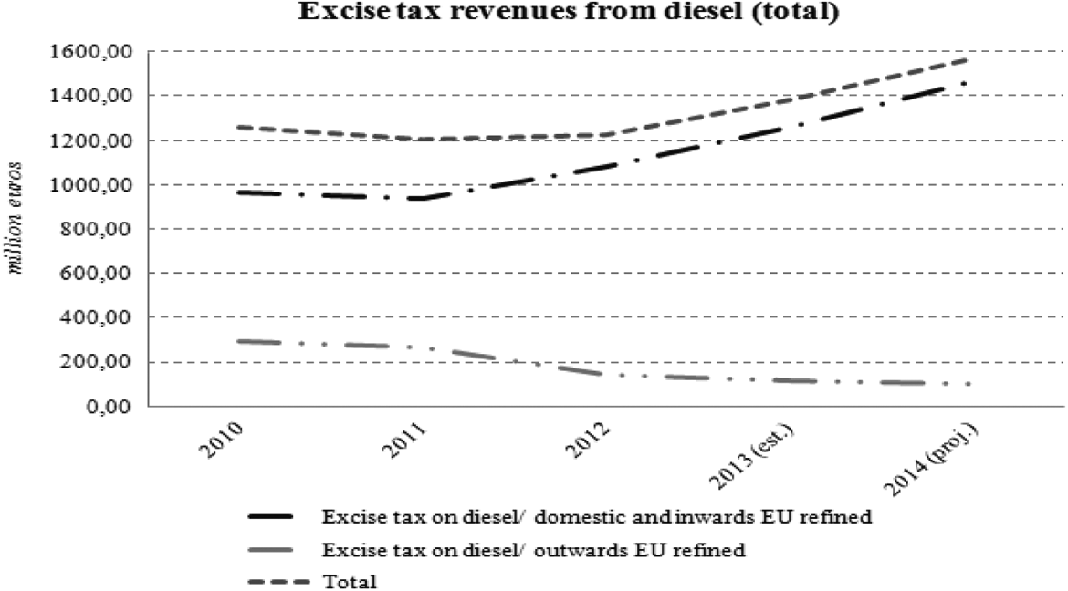
Excise tax revenues from diesel (no disaggregation between heating and automotive diesel).
However, actual MoF consumption data confronted this view by picturing a slowdown in diesel consumption in both markets (figure 3). Automotive diesel consumption dropped from 420,000 tons in 2008 to 280,000 tons in 2012. Heating diesel consumption, starting from 800,000 tons also dropped to less than 600,000 in 2012, and following the admittedly favorable weather conditions to less than 250,000 tons in 2013. Lastly, during the period under examination (after 2009), the price pattern for both Greek heating diesel and automotive diesel moved upward (figure 4) following the global oil price increase.
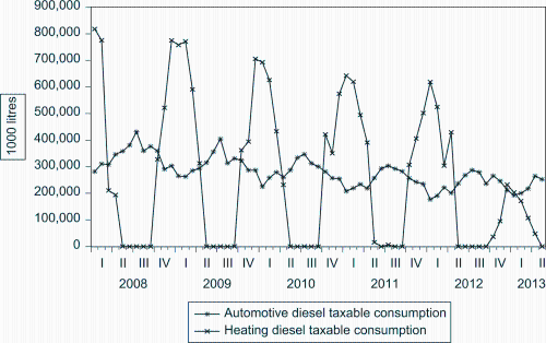
Diesel taxable consumption in Greece (tones: 1,000 liters).
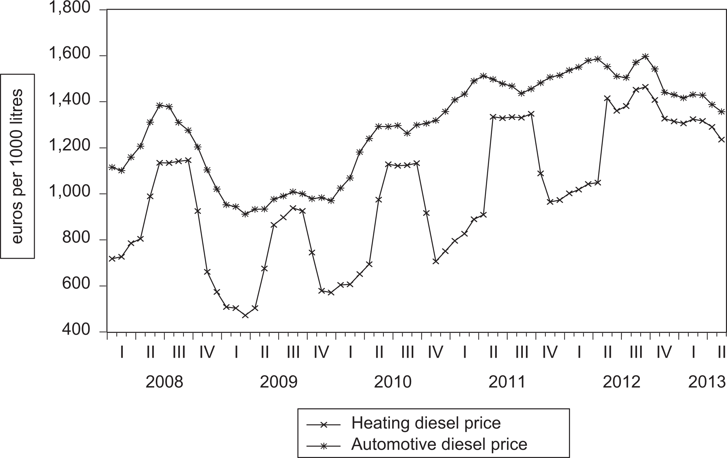
Diesel price level in Greece (euros per 1,000 liters).
Model Specification
In this analysis, a structural linear demand model is applied to investigate the heating and automotive diesel markets due to the limited span of the data. For consistency’s sake, the empirical analysis also applies alternative specifications of partial adjustment models (i.e., Hughes, Knittel, and Sperling 2008). This is done by including lagged consumption effects (Dht , Dat ) to linear structural demand models.
As the main policy target of the end-2012 excise tax reform has been its effectiveness to tackle arbitrage between the two diesel markets, the standard demand specification is extended to capture any possible arbitrage effects. This is made possible by applying Polemis’s (2006) approach of including cross-price elasticities to investigate the degree of substitutability between energy markets (i.e., gasoline and diesel market). More specifically, in the right-hand side of the heating diesel demand equation, the retail price of automotive diesel (Da_pt/coef .a4) is included. The automotive diesel demand equation is also augmented in the right-hand side by the heating diesel retail price (Dh_pt/coef .β4). To simplify the interpretation of the results, excise tax is deducted from gross prices.
More specifically, the following heating diesel demand is considered:

In the case of automotive diesel demand, an analogous representation is followed:

Explanatory variables used in equations (1) and (2) are as follows: Dht and Dat denote taxable quantities of heating diesel and automotive diesel consumption. Dh_pt and Da_pt denote retail prices, Yt denotes disposable income, and lastly t_ht and t_at also refer to excise tax (defined as the total excise tax charge levied on the quantity of diesel at the time of release for consumption). Following, Karavitis, Maniatis, and Danchev (2012), the heating degree day index denoted by hddt is also used to capture interactions between exogenous weather conditions and diesel demand. hbt denotes the reimbursed heating benefit for heating diesel consumption after the 2012 tax equalization reform. Dummy d2012m12 accounts for potential demand shifts before and after the common tax rate introduction. It is defined as a step dummy equal to 1 after October 2012 and 0 otherwise. With the exception of variable hbt , all variables enter in logs, allowing elasticity interpretation of empirical findings.
To test if arbitrage exists from the cheaper (i.e., lower excise taxation) to the more expensive diesel market (i.e., higher excise taxation), two separate hypothesis tests are needed. Firstly, the automotive diesel retail price makes a positive and significant contribution to heating diesel demand (coef .a4). Secondly, the heating diesel retail price has an insignificant impact on automotive demand (coef .β4).
In an analogous way, the implications of arbitrage from the 2012 common rate reform may also be tested by focusing on the relevant dummy cross-product variables. More specifically, a negative and significant interaction coefficient (coef .a8) in the heating diesel equation (1) and an insignificant (coef .β6) in the automotive diesel equation (2) are indicative of an arbitrage limitation following the introduction of the common excise tax.
Lastly, when estimating demand and supply equations over a long period through least square (LS), a common limitation relates to the joint determination of price and quantity due to supply and demand shifts. In this case, estimates may be biased and inconsistent as the price and error term may be correlated. This limitation is overcome by applying the Belhaj (2002), Sharma, Chandramohanan Nair, and Balasubramanian (2002), and Nicol (2003) approach that follows a simultaneous 3SLS system approach. The demand functions of the two interrelated diesel markets are jointly estimated while the lagged demand regressors are used as instruments. The robustness checks of the empirical findings are based on the generalized method of moments (GMMs).
Data Description
The monthly data used in the article come from a number of official sources and stretch from January 2008 up to May 2013. Taxable heating and automotive diesel consumption (Dht and Dat) refer to unpublished MoF administrative data. The same data source is used for the levels of excise taxation in both diesel markets. These are expressed in Euros per 1,000 liters (t_ht and t_at). Retail prices for heating and automotive diesel per 1,000 liters (Dh_pt and Da_pt) come from the EC Oil Bulletin and are inclusive of taxation and excise duties. The same source is also used for the heating degree day (hddt )variable that captures heating needs in a specific period. 11 Finally, the heating benefit hbt (expressed in Euros reimbursed to households per 1,000 liters) and the disposable income Yt were provided by the Hellenic Foundation for Economic and Industrial Research. The descriptive statistics for the sample data are presented in table A1 of the appendix.
Estimation Results
Single Equation Estimates
Previous demand models are estimated using LS controlling also for potential autocorrelation effects. In the case of the heating diesel market, it is noted that the market is operational during the heating period, that is, November these April. Following those constraints, the analysis is based on two sets of output estimates: firstly, estimates that refer to the heating period for which the heating diesel market is operational and secondly, the full-year (twelve-month) estimates, which are more appropriate for the automotive diesel market.
Table A2 presents estimation results for the heating diesel demand model during the heating period across alternative specifications of the static and the partial adjustment demand model. The model across all specifications fits the data well (i.e., adjusted R 2: .77–.89, regression equation specification error test [RESET] p value: .15–.60, Breusch-Godfrey [Lagrange multiplier, LM] p value: .40–.60, and Gleizer p value: .15–.26).
Coefficient estimates for price and income elasticity have the expected signs with coefficients (a 1 and a 2) varying between −0.61 and −0.67 and 0.88 and 0.94, respectively, supporting a highly elastic demand in the case of the Greek heating diesel market (columns 1–6). Tax elasticity is also negative and significant (coef .a3, highlighted), ranging from −0.33 to −0.39 in all demand representations. Furthermore, a strongly positive and statistically significant contribution of the automotive diesel price on heating diesel demand (coef .a4) is observed across all specifications with above unity elasticity estimates. The high value of this coefficient pictures a strong substitution between the two diesel markets. Moreover, the relevant dummy interaction term (coef .a8) is insignificant, suggesting that substitution between markets remained unchanged after 2012 when the excise tax reform took place.
A limited impact of the benefit for heating diesel demand in Greece is also found, as the relevant estimate (coef .a5) is insignificant for heating diesel demand. This should be attributed to the design of the scheme as it aimed to support mainly peripheral regions in Greece. These regions face extreme winter conditions and are usually scarcely populated and thus represent a relatively lower share of total heating diesel consumption. On the other hand, the more populated urban areas of Greece that represent a relative larger part of total consumption are entitled to a lower benefit supporting the insignificant effect of the heating benefit for total heating diesel demand.
Heating degree day hddt elasticity is positive and significant (+0.68), pointing to the importance of heating needs, and weather conditions in general, for diesel heating demand. On the contrary, the d2012m12 dummy is statistically insignificant, rejecting the scenario of demand shifts after the introduction of the common rate for the two diesel markets.
Moreover, as a robustness test the estimation period is limited to December 2012, to avoid possible outlier effects from the large increase in excise heating diesel tax (450 percent) after 2012. Again, the obtained estimates (columns 7–9, table A2) are similar to previous results. Lastly, in all representations the potential effects from other substitute energy markets, that is, the electricity and gas markets (liquefied and nonliquefied) are also accounted for. Under all estimations, their influence on the heating diesel demand is negligible. 12
Table A3 shows relevant results for the automotive diesel demand. Following these, the employed linear demand framework provides a satisfactory fit for the demand model (i.e., adjusted R 2: .81–.90, RESET p value: .12–.41, Breusch-Godfrey (LM) p value: .24–.40, and Gleizer p value: .16–.33). Full-year estimates reflect a less responsive demand with respect to price and income variations against the heating diesel market, as elasticities are significant though smaller, ranging from −0.35 to −0.48 (coef.β1) in the first case and from +0.28 to +0.32 in the second case (coef.β2). These estimates are comparable with the demand elasticities of Coyle, DeBacker, and Prisinzano (2012) and Porcher and Porsher (2014) in the case of automotive diesel markets in the United States and France. Equally as in the case for heating diesel, the excise tax estimate is negative and significant (coef.β3, highlighted), with lower elasticities compared to the heating diesel case, ranging from −0.22 to −0.29.
Moreover, the statistical significance of the heating diesel price on diesel automotive demand (coef .β4) varies in terms of sign and significance across different specifications and estimation outputs. This hazy result is further examined in the next section. The relevant interaction term (coef .β6), capturing the post-2012 heating diesel price impact on the automotive diesel demand, is also insignificant.
When accounting for potential seasonality effects 13 in the automotive diesel model, statistically significant seasonal dummies refer to the winter period during which the heating diesel market operates. This seasonality pattern in the Greek automotive diesel market emphasizes linkages with the heating diesel market. The estimation period is limited to December 2012 to test for any outlier effect from the significant drop (30 percent) in automotive excise taxation, after the 2012 reform. The same as before, the findings of the automotive diesel determinants again remain unchanged (columns 5–8).
Simultaneous Equation Estimates
This subsection presents the system estimation results. System estimates for both demand equations limited to the heating period only (November–April) are presented in table A4. In principle, heating diesel elasticities (upper part of table) are close to the LS estimates (columns 1–4). Price and income have a significant impact on signs and elasticities (coef.a1), ranging between −0.5 and −0.6 in the first instance and between (coef.a2) +0.91 and +1.06 in the second one. Again, the excise taxation effect (coef.a3, highlighted) is in line with the LS estimates. All these estimates show a negative and significant contribution that ranges from −0.37 to −0.41 across all specifications (columns 1–4). Also the estimated insignificant impact of the heating benefit on diesel consumption is in line with the previous univariate findings (coef.a5). Weather conditions variable, as expressed by heating degree days (hddt), also represents a significant and robust determinant of heating oil demand with an impact varying between +0.31 and +0.37.
The lower part of table A4 refers to the automotive diesel demand function. Price and income elasticities exhibit the usual sign and are significant across different specifications. Following 3SLS and GMM estimates (columns 1–4), price (coef.β1) and income elasticities (coef.β2) vary between −0.62 and −0.68 and between +0.12 and +0.20, respectively. Excise taxation (coef.β3, highlighted) has a negative, significant though lower (compared to heating diesel estimates) contribution, ranging between −0.24 and −0.27 across alternative specifications and estimation methodologies. Following previous robustness tests, the original demand models are reestimated, limiting the period to end-2012. As seen in columns 5 through 8, variables of interest provide estimates that are close to the full period estimates.
Lastly, table A5 provides system estimates for the demand equation over the full year. Since the heating diesel market is nonoperating through the entire period, the findings and analysis focus only on estimates for the automotive diesel demand model (lower part of table).
The estimation results confirm previous findings for automotive diesel. Price elasticities are higher under both estimation system methods, varying between (coef.β1) −0.57 and −0.68. Income contributes at a marginally lower level compared to the LS estimates, ranging between (coef.β2) +0.10 and +0.17. The previous findings of a negative and significant excise taxation elasticity (coef.β3, highlighted) are also confirmed with estimates ranging from −0.23 to −0.29. When limiting the estimation period to end-2012, consistent estimates of price and income elasticities with full period estimates (columns 5–8) are acquired.
Policy Implications of the 2012 Excise Tax Reform
Building on previous empirical findings, this part of the analysis presents the policy implications of the 2012 Greek excise tax reform. These focus on the initial policy reform targets set by MoF, that is, the limitation of the arbitrage between diesel markets and also the increase of excise tax revenues.
Arbitrage Implications
The LS estimates (tables A2 and A3) on the effect of cross-market prices (coef.a4 and β4), that is, heating and automotive diesel prices on automotive and heating diesel demand, respectively, proved unsuccessful to provide a robust view of arbitrage between the diesel markets under scrutiny.
On the contrary, following a simultaneous equation framework, findings from tables A4 and A5, provided evidence of an arbitrage pattern from the “cheaper” heating diesel to the “expensive” automotive diesel market. More specifically, the estimation results point to a positive and significant contribution of the automotive diesel price level (coef.a4) on heating demand. Estimates vary between +2.2 and +2.9 (coef.a4), and these are coupled with an insignificant effect of the heating diesel price (coef.β4) to automotive diesel demand (equation (2)). These findings suggest that in the context of interrelated energy markets as the case of the Greek diesel markets, arbitrage relations are more effectively captured in a simultaneous system context that allows the joint determination of prices and quantities in interrelated markets and thus keeps the simultaneity bias to a minimum.
Moreover, coefficients a8 and β6 remain insignificant under different specifications. Based on the economic interpretation of these estimates, after the 2012 tax reform, no sign of arbitrage limitation exists. The observed slow adjustment of the Greek diesel markets, following the common tax rate adoption provides evidence that when it comes to limiting arbitrage, fiscal policy gains remain more of a medium-term nature. Even though country specific, the reasons why “common rate” fiscal policies are not immediately effective in tackling arbitrage between substitute markets may include significant stock build ups (i.e., of heating diesel in the case of Greek diesel market) and the medium-term horizon of other supporting tax “administration” reforms, which are essential to effectively tackle arbitrage between markets, that is, the obligation of GPS devices for tracks transporting diesel, the electronic book keeping of quantities merchandised, the intensification of high way inspections, the stricter code of fines for those involved in arbitrage, and so on.
Budgetary Implications
Adopting a common excise tax rate between substitute energy markets may also lead to positive budgetary implications by increasing tax collections. Such a scenario is possible if the proper tax rate applies to markets of different magnitudes and excise tax elasticities. Using the estimated excise tax elasticities for the Greek diesel markets, revenue changes from the common tax rate introduction may be simulated on a ceteris paribus basis.
Ceteris paribus, formula (3) approximates the one period forward revenue percentage change (%ΔR) with excise tax rate percentage change (%Δτ) adjusted by the excise tax rate elasticity 14 (coef.a3, β3 denoted by eτ→q). Using this formula, the one year forward revenue collection may be simulated for different levels of excise tax rate in every diesel market.

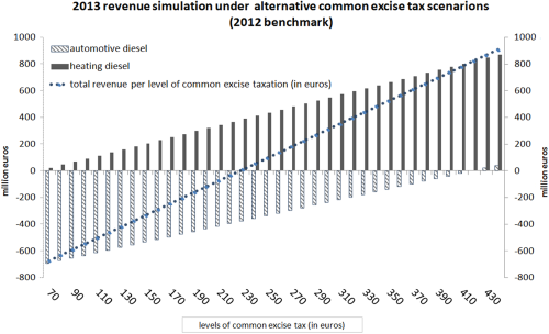
Setting the 2012 total excise tax revenue collections 15 as a reference for both markets, figure 5 provides simulated collections of excise tax for each diesel market across different levels of common excise tax rates introduced at end-2012. Following these, equalizing the diesel taxation at €330 per 1,000 liters leads to an increase of total excise tax revenues by €384 million in the first year of the reform, that is, 2013.
Simulated revenues.
This is the result of a revenue increase of €563 million for the heating diesel market and a revenue loss of €179 million for the automotive diesel market. In the latter automotive diesel market, the simulated excise tax collection increase is close to the 2013 actual realizations 16 as following the MoF, revenue collections from this side were reduced by €120 million in 2013.
The observed difference in the former heating diesel market between the simulated and the actual excise tax collections (i.e., increase of €170 million in 2013 according to the MoF) reflects the ceteris paribus nature of simulation formula (3). In this respect, the total budgetary outcome of the reform should be considered the result of a number of factors, that is, the direct discretionary fiscal impact of the reform, income evolution, weather conditions, and lastly, and more importantly, arbitrage that continues to contract the tax base and reduce tax collections after the 2012 reform as previously proved.
As seen in figure 5, following formula (3) simulation the breakeven excise tax rate between total revenue gains and losses is approximately at €230/1,000 liters lower than the adopted common rate of €330/1,000 liters This means that the 2012 tax reform aimed from the outset to the increase of revenues. Lastly, it follows from the analysis that if the current common rate regime is abolished through the reduction of the excise tax rate in at least one of the diesel markets, then all other things equal, on top of the negative arbitrage implications, a loss of revenues is likely to occur.
Conclusions
This article explores the fiscal implications of the 2012 excise tax reform in Greece, which adopted a common excise tax rate between heating and automotive diesel. The empirical analysis uses unpublished administrative data for taxable consumption in both diesel markets and follows single and system empirical estimation methods that account for cross-market dependencies.
In summary, empirical findings suggest a more elastic heating diesel demand with respect to price and excise taxation variations compared to the relevant automotive diesel market. Moreover, it is proved that in the context of substitute energy markets (e.g., Greek diesel markets), arbitrage relations are more effectively captured in a system context that accounts for the joint determination of prices and quantities. Following this approach, no support of an arbitrage limitation in these diesel markets is found after the 2012 adoption of the common excise tax rate.
These findings suggest that, in terms of limiting arbitrage though price convergence, fiscal policy gains take longer to materialize. The main reasons for this slow market adjustment could be the presence of a significant stock accumulation of heating diesel before 2012 and the medium-term horizon of relevant tax administration reforms that are also essential to support the 2012 common excise tax rate reform in the Greek diesel market.
Finally, the ceteris paribus revenue simulation in the case of the Greek diesel market suggests that it is possible for a well-designed excise tax rate to pursue both the limitation of arbitrage and the increase of tax revenues. Necessary conditions for this is, firstly, the adopted common excise tax rate is set above a certain threshold (“breakeven point” as expressed in this analysis), and secondly, and not least important, the supporting tax administration reforms gain significant momentum.
Footnotes
Appendix
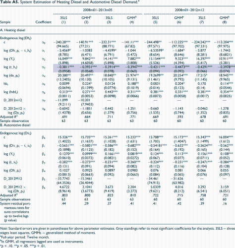
System Estimation of Heating Diesel and Automotive Diesel Demand.a
| Sample | Coefficient | 2008m01–2013m05 | 2008m01–2012m12 | ||||||
|---|---|---|---|---|---|---|---|---|---|
| 3SLS | GMMb | 3SLS | GMMb | 3SLS | GMMb | 3SLS | GMMb | ||
| (1) | (2) | (3) | (4) | (5) | (6) | (7) | (8) | ||
| A. Heating diesel | |||||||||
| Endogenous: log (Dht) | |||||||||
| c | α0 | −240.28*** (94.665) | −140.91*** (77.21) | −232.31*** (88.771) | −141.11*** (67.82) | −244.498** (97.571) | −112.225*** (97.702) | −234.242*** (97.331) | −113.204*** (97.975) |
| log (Dh_pt − t_ht) | α1 | −5.4569* (8.785) | −1.0383 (6.471) | −4.4599* (6.791) | −1.044 (5.472) | −6.53599* (8.654) | −1.684* (8.646) | −5.877 (8.281) | −1.7443 (8.6821) |
| log (Yt) | α2 | 16.049*** (5.898) | 9.842*** (4.6058) | 14.141*** (5.898) | 7.882*** (3.808) | 15.1544*** (5.526) | 9.323*** (4.394) | 16.397*** (5.417) | 10.911*** (5.281) |
| log (t_ht) | α3 | −0.3811*** (0.0958) | −0.3931*** (0.0568) | −0.3914*** (0.078) | −0.3947*** (0.060) | −0.4211*** (0.094) | −0.4473*** (0.092) | −0.4291*** (0.066) | −0.3978*** (0.074) |
| log (da_pt) | α4 | 20.380** (13.2405) | 20.497** (10.130) | 18.840** (10.105) | 21.974** (9.131) | 19.2699** (11.461) | 20.254*** (9.792) | 17.215* (11.145) | 18.945*** (9.965) |
| hbt | α5 | 0.0099 (0.0694) | 0.224* (0.1399) | 0.0124 (0.0774) | 0.188** (0.1019) | 0.0031 (0.014) | 0.204* (0.123) | 0.170 (0.14) | 0.114*** (0.0544) |
| log (hddt) | α6 | 0.313*** (0.0011) | 0.271*** (0.0053) | 0.443*** (0.0098) | 0.311*** (0.0066) | 0.381*** (0.0073) | 0.331*** (0.0058) | 0.381*** (0.0017) | 0.354*** (0.0025) |
| D_2012m12 | α7 | −11.099 (9.2111) | −10.201 (7.9403) | — | — | — | — | — | — |
| D_2012m12 × log (Da_pt) | α8 | −0.6042 (1.4378) | −1.1851 (0.656) | −0.442 (1.379) | −1.251 (0.756) | −0.660 (1.535) | −1.143 (0.744) | −0.0462 (1.352) | −1.278 (0.835) |
| Adjusted R 2 | .691 | .664 | .711 | .771 | .669 | .593 | .678 | .691 | |
| Sample observation | 63 | 63 | 63 | 63 | 60 | 60 | 60 | 60 | |
| B. Automotive diesel | |||||||||
| Endogenous: log (Dαt) | |||||||||
| c | β0 | 15.326*** (1.4022) | 15.735*** (1.1637) | 15.261*** (1.1028) | 15.233*** (1.631) | 15.708*** (1.703) | 15.173*** (1.4047) | 15.343*** (1.1499) | 16.004*** (1.612) |
| log (Dα_pt − t_αt) | β1 | −0.5651*** (0.1898) | −0.5801*** (0.1125) | −0.586*** (0.182) | −0.682*** (0.152) | −0.54181*** (0.164) | −0.632*** (0.192) | −0.5624*** (0.165) | −0.562*** (0.144) |
| log (Yt) | β2 | 0.1270*** (0.0610) | 0.0999*** (0.0372) | 0.1661*** (0.0821) | 0.0819*** (0.0272) | 0.124*** (0.067) | 0.113*** (0.077) | 0.1561*** (0.0711) | 0.108*** (0.052) |
| log (t_αt) | β3 | −0.282*** (0.131) | −0.273*** (0.091) | −0.231*** (0.094) | −0.260*** (0.082) | −0.224*** (0.112) | −0.231*** (0.116) | −0.2471*** (0.104) | −0.284*** (0.128) |
| log (Dh_pt) | β4 | 0.1027 (0.0813) | 0.0925 (0.0663) | 0.0897 (0.092) | 0.0983 (0.0663) | 0.076 (0.084) | 0.081 (0.065) | 0.066 (0.076) | 0.055 (0.097) |
| D_2012M12 | β5 | −33.7743 (64.3536) | −15.3461 (26.4044) | — | — | −34.461 (74.915) | −31.626 (63.982) | — | — |
| D_2012M12 × log (Dh_pt) | β6 | 4.6722 (8.9614) | 2.1041 (3.6773) | 3.673 (9.419) | 2.204 (3.273) | 5.0339 (9.621) | 4.016 (8.212) | 3.292 (6.541) | 3.159 (6.051) |
| Adjusted R 2 | .803 | .800 | .823 | .810 | .722 | .715 | .758 | .721 | |
| Sample observations | 63 | 63 | 63 | 63 | 60 | 60 | 60 | 60 | |
| System residual portmanteau tests for auto correlations up to twelve lags (p value) | .44 | .29 | .37 | .41 | .41 | .42 | .39 | .16 | |
Note: Standard errors are given in parentheses for above parameter estimates. Gray standings refer to most significant coefficients for the analysis. 3SLS = three stages least squares, GMMs = generalized method of moments.
aFull-year period: Twelve month.
bIn GMM, all regressors lagged are used as instruments.
*p < .10. **p < .05. ***p < .01.
Author’s Note
Any remaining errors or shortcomings in this article are those of the author. The views expressed in this article are those of the author and do not necessarily reflect those of the European Central Bank, the European System of Central Banks, or the Bank of Greece.
Acknowledgments
I gratefully acknowledge comments and suggestions from Elias Tzavalis, Dafni Nikolitsa, Athanassios Tangalakis, Sylvia Baudet von Gersdorff, the two anonymous referees, and the editor of Public Finance Review.
Declaration of Conflicting Interests
The author(s) declared no potential conflicts of interest with respect to the research, authorship, and/or publication of this article.
Funding
The author(s) received no financial support for the research, authorship, and/or publication of this article.