An Examination of Power and Type I Errors for Two Differential Item Functioning Indices Using the Graded Response Model

Abstract

This study examined two methods for detecting differential item functioning (DIF): Raju, van der Linden, and Fleer’s 1995 differential functioning of items and tests (DFIT) procedure and Thissen, Steinberg, and Wainer’s 1988 likelihood ratio test (LRT). The major research questions concerned which test provides the best balance of Type I errors and power and if the tests differ in terms of detecting different types of DIF. Monte Carlo simulations were conducted to address these questions. Equal and unequal sample size conditions were fully crossed with test lengths of 10 and 20 items. In addition, α and β parameters were manipulated in order to simulate DIF. Findings indicate that DFIT and LRT both had acceptable Type I error rates when sample sizes were equal but that DFIT produced too many Type I errors when sample sizes were unequal. Overall, the LRT exhibited greater power to detect both α and β parameter DIF than did DFIT. However, DFIT was more powerful than LRT when the last two β parameters had DIF as opposed to when the extreme β parameters had DIF.

Keywords

computer simulation procedures Monte Carlo bootstrapping item response theory ANOVA methods

Differential item functioning (DIF) is an important research topic for psychologists because people with the same underlying ability from different groups may have different probabilities of endorsing the same item. DIF analyses have been used in several different ways in organizational research. One way is to develop tests and scales that have measurement equivalence across subgroups. In these situations, DIF analyses can be used to identify problem items that can be removed from the scale. A second use of DIF analyses has been to assess the measurement equivalence of existing scales across groups or situations. For example, researchers have used DIF to examine differences between male and female respondents (e.g., Braddy, Meade, & Johnson, 2006; Collins, Raju, & Edwards, 2000), different test versions (e.g., Donovan, Drasgow, & Probst, 2000), and racial differences (e.g., Braddy et al., 2006; Collins et al., 2000; Raju, Laffitte, & Byrne, 2002). Finally, DIF analyses can be used to test interesting hypotheses about item responding. For example, Robie, Zickar, and Schmit (2001) investigated faking on personality assessments by comparing applicants and incumbents using DIF analyses.

These various studies involving DIF have allowed researchers to answer a variety of research questions. Thus, it is important that researchers are able to use DIF techniques that perform accurately. A number of different DIF techniques have been developed. Some examples of these different methods include the area between two item response functions (IRF; Raju, 1988, 1990); Lord’s (1980) χ² test; the Mantel-Haenszel technique (Holland & Thayer, 1988); the delta method (Angoff & Ford, 1973); the differential functioning of items and tests (DFIT) procedure (Raju, van der Linden, & Fleer, 1995); and Thissen, Steinberg, and Wainer’s (1988) likelihood ratio test (LRT). Of these, the DFIT and LRT appear to be the most frequently used in organizational research (e.g., Collins et al., 2000; Donovan et al., 2000; Henry & Raju, 2006; Maurer, Raju, & Collins, 1998; Morales, Flowers, Gutierrez, Kleinman, & Teresi, 2006; Raju et al., 2002; Stark, Chernyshenko, Drasgow, & Williams, 2006). Unfortunately, there has been a lack of empirical work comparing the performance of these two tests, and it is not clear which should be preferred under certain circumstances.

In the present study, we examined the Type I error rates and power of the DFIT framework (Raju et al., 1995) and the LRT (Thissen et al., 1988) using the graded response model (GRM). We manipulated a number of conditions in order to identify which fit index should be preferred overall for DIF detection and whether different indices capture different sources of DIF. In the following sections, we briefly review the GRM that is often used to analyze polytomous items and then describe the two DIF indices.

Graded Response Model

In many situations, researchers use polytomous Likert-type scale items with more than two response options. Samejima’s (1969) GRM has been typically applied to analyze this type of item data. The GRM assumes that an item has m ordered categories. Estimates are based on m – 1 boundary response functions (BRFs). Each BRF represents the cumulative probability of selecting a response option greater than the option of interest. For example, a Likert-type scale with five response options would have four BRFs. The first BRF is the probability of choosing the lowest response option versus the cumulative probability of choosing the other four options. The second BRF is the probability of choosing the lowest two response options versus the probability of choosing the other three, and so on. The equation for a BRF is

\frac{P_{i k}^{*} (Y = 1 | θ) = {e x p [α}_{i} (θ - β_{i}_{k})]}{1 + {e x p [α}_{i} (θ - β_{i}_{k})]}

In this equation, α_i is the item discrimination parameter, β_ik is a difficulty parameter for option k, and θ is the ability parameter for the individual. There are m – 1 threshold parameters. For example, the β_ik difficulty parameter for choosing greater than the lowest option represents the point on the θ scale where there is 50% probability that the response is greater than the lowest option. Using Equations 2 through 6, the probability of responding to each of the five categories (P_i ₁ to P_i ₅) may be calculated.

P_{i 1} (θ) = 1 - P_{i 1}^{*} (θ),

P_{i 2} (θ) = P_{i 1}^{*} (θ) - P_{i 2}^{*} (θ),

P_{i 3} (θ) = P_{i 2}^{*} (θ) - P_{i 3}^{*} (θ),

P_{i 4} (θ) = P_{i 3}^{*} (θ) - P_{i 4}^{*} (θ),

and

P_{i 5} (θ) = P_{i 4}^{*} (θ) - 0.

After the probability of responding to each of the five categories is estimated, a measure of the expected item score can be calculated. For polytomous data, an expected score (ES_si ) can be calculated for examinee s on item i as

E S_{s i} = \sum_{k = 1}^{m} P_{i k} (θ_{s}) X_{i k},

where X_ik is the score for category k, m is the number of categories, and P_ik is the probability of responding to category k. Put simply, the expected score is the sum of the product between the probability of endorsing a response option and the value of the response option. Summing the expected scores across a test will result in an expected test score function,

T_{s} = \sum_{i = 1}^{n} E S_{s i},

where n is the number of items on the test.

The Differential Functioning of Items and Tests Framework

The DFIT procedure includes three measures: differential test functioning (DTF), compensatory DIF (CDIF), and noncompensatory DIF (NCDIF). The DFIT indices allow for the determination of whether individual items exhibit DIF (CDIF and NCDIF) and/or whether the test as a whole functions differently (DTF). The DTF index is based on the notion that although individual items may function differentially, these differences can cancel each other out across items, so the test may not exhibit DTF. If there is no DTF and the researcher is not worried about individual-item DIF, then all of the items in the test may remain. The DTF index is defined as the average squared difference between the true test score functions for the focal and reference groups. For a polytomous model, the difference is based on comparing the expected test scores of examinees using the focal and reference groups' item parameters, respectively:

D (θ_{s}) = T_{F} (θ_{s}) - T_{R} (θ_{s}),

where T _F is the expected test score based on the focal group’s parameters, and T _R is the expected test score based on the reference group’s parameters. DTF is the expected value of the squared difference between the focal and the reference groups across the θ distribution from the focal group (E _F):

D T F = E_{F} [D (θ_{s})^{2}] .

CDIF and NCDIF are the two item-level DIF indices in the DFIT framework. One can use the CDIF index to identify items that contribute to DTF. Under this index, all of the items on the test are considered, and items that if removed would lower DTF are noted. When one sums CDIF values across items, the outcome is equal to DTF. CDIF can be calculated by finding the covariance of D and d (the probability of success on an item for a person in the focal group and the probability of success on an item for a person in the reference group) and adding that to the product of the mean of d and the mean of D :

{C D I F}_{i} = C o v (d_{i}, D) + μ_{d i} μ_{D} .

The NCDIF index can be used to identify individual items exhibiting DIF independent of other items on the test. This means that NCDIF will flag an item even if the item’s DIF is canceled out at the test level. NCDIF is similar to DTF except that it is based on comparing expected item scores among focal group respondents' expected scores using focal group item parameters versus reference group item parameters. The NCDIF index is the expectation over the focal group (E _F) of squared differences between the probability of endorsing an item using the focal item parameters, P_i _F(θ), and the probability of endorsing an item using the reference group parameters, P_i _R(θ). If d_i equals the difference between the expected item scores under the focal and reference group parameters, then

{N C D I F}_{i} = E_{F} [E_{s i}_{F} (θ {) - E}_{s i R} (θ {)]}^{2} = E_{F} (d_{i})^{2} = σ_{d i}^{2} + μ_{d i} 2,

where σ and μ are the standard deviations and means, respectively, of d_i .

Item Parameter Replication Method

Raju et al. (1995) originally proposed χ² tests to evaluate the statistical significance of the DTF and NCDIF indices. However, these tests tended to commit too many Type I errors. The focus then shifted to establishing cutoff values for the two indices. Raju et al. and Flowers, Oshima, and Raju (1999) proposed overall cutoff values of .006 and .016, respectively, for the NCDIF index. However, these cutoff values were not generalizable to other items and were also specific to the item response theory (IRT) model being used. Empirically derived cutoff values for the NCDIF index have been explored, and research has generally supported their use. Several studies have found acceptable Type I errors and reasonable power for overall empirical cutoffs (Bolt, 2002; Flowers et al., 1999; Meade, Lautenschlager, & Johnson, 2007). However, despite the promise in using empirically derived cutoff values, most researchers have neither the expertise nor the time to do these sorts of calculations. To address this, Oshima, Raju, and Nanda (2006) developed the item parameter replication (IPR) method for use with dichotomous data. This method has been extended recently to polytomous data (Raju et al., 2009).

The IPR method utilizes estimates of item parameters for the reference group, as well as variances and covariances for those estimates, in order to obtain a distribution of NCDIF values that can be rank ordered. Based on these estimates, a number of replications of item parameters are then generated using the same sampling variance and covariance as the original item parameters. This assumes that any differences between the original parameters and the newly generated parameters are due to sampling error. After a large number of replications are complete, an empirical sampling distribution of NCDIF under the null hypothesis that both groups (the focal and reference) are equal is produced.

The IPR method has been a fairly recent addition to the DFIT framework. As such, most of the existing research on the DFIT framework does not use this method. In particular, the empirical evaluations of Type I errors and power (e.g., Bolt, 2002; Meade et al., 2007) predated its development. Thus, it is not clear how well the IPR method performs in terms of Type I errors and power. One potential problem with the IPR method is that it assumes that the item parameter estimates' variances and covariance for the reference group generalize to the focal group. This assumption may be violated when the sample sizes for the two groups differ, as sample size will likely affect the variances of the item parameters. In the present study, we assessed the magnitude of the effect of unequal sample sizes on the evaluation of the extent of DIF for a set of items.

The Likelihood Ratio Test

The LRT is based on comparing the relative goodness of fit of nested models and can be implemented in two ways (e.g., Rivas, Stark, & Chernyshenko, 2009; Stark et al., 2006; Wang, 2004; Wang & Yeh, 2003). One way is the constrained baseline method where a baseline model is formed by constraining all item parameters to be equal across groups. DIF is detected by estimating a series of comparison models by freeing the item parameters one item at a time. The second method is called the free baseline method where the baseline model is formed by freeing all of the item parameters except a referent subset of items. Comparison models are formed constraining the item parameters to be equal across groups. Again, this is done item by item.

Research suggests that the free baseline method results in lower Type I error rates and more power compared with the constrained baseline method (Stark et al., 2006; Wang & Yeh, 2003). In addition, Rivas et al. (2009) found that using highly discriminating items as anchors improved performance. Based on this, we used the free software program IRTLRDIF 2.0 (item response theory likelihood ratio differential item functioning; Thissen, 2001) to conduct LRTs using the free baseline method.

Under the free baseline method, the user specifies a set of anchor and candidate items. The anchor items are items that the researcher believes do not exhibit DIF. Rivas et al. (2009) found that a single highly discriminating item can be an effective anchor item when large amounts of DIF are present, and additional anchor items increase power for detecting smaller amounts of DIF. Candidate items are the items that are tested for DIF. A series of augmented models are formed by constraining the item parameters of the candidate items to be equivalent across groups. This is done item by item. The fit of the baseline and augmented models is compared using a likelihood ratio test:

G^{2} (d f) = - 2 log [\frac{L [A]}{L [B]}],

where L represents the likelihood of the data given the maximum likelihood estimates of the parameters of the model, A refers to the augmented model, and B refers to the baseline model. G ² is distributed as a χ² with degrees of freedom equal to the difference between the number of parameters in the augmented model and the number of parameters in the baseline model. The LRT essentially tests the equivalent of the item parameters across groups.

Research on DFIT and LRT

The DFIT framework and LRT have been two of the most frequently used ways of testing for DIF, and there has been some research investigating their performance. For example, numerous studies have shown the DFIT framework to be successful at detecting items and tests that may be biased (e.g., Flowers et al., 1999; Meade et al., 2007; Raju et al., 1995). A number of researchers have examined the LRT and have shown that the test has enough power to detect DIF at the item level (e.g., Ankenmann, Witt, & Dunbar, 1999; Kim & Cohen, 1998; Thissen et al., 1988).

Little research has directly compared the NCDIF index with LRT. One exception is Bolt’s (2002) study. He generated 30 items with three different IRT models, the GRM, the generalized partial credit model, and the two-parameter sequential response model for sample sizes of 300 and 1,000. Type I error rates for the LRT were in the acceptable 5% range when Bolt used the GRM to generate the data but went up to 20% when the model was misspecified. Type I error rates for the NCDIF index were acceptable regardless of the generating model. Both procedures had acceptable power across most conditions, but the LRT exhibited more power overall than did the NCDIF index. It is important to note that Bolt’s study did not include the IPR method for the NCDIF index or the free-baseline LRT.

Braddy et al. (2006) also compared the DFIT framework and LRT directly. They found that the DFIT procedure indicated that the test as a whole did not have DTF and only identified 1 item in all of the conditions as DIF. In contrast, the LRT identified 10 DIF items. These results do not indicate which DIF detection method was more accurate at assessing DIF because the true magnitude of population DIF in this study was unknown. The different conclusions implied from Braddy et al.’s study indicate that it is crucial to know which of these fit indices to use in order to avoid producing a test with extensive DIF. Thus, there are still a number of questions concerning which DIF test should be preferred overall and how various conditions affect the DIF tests.

Present Study

In the present study, we examined the Type I error rates and power for the NCDIF index using the IPR method and the free-baseline LRT across a number of conditions. Specifically, we varied the test length and source of DIF by manipulating the discrimination and threshold parameters. We were interested primarily in (a) how the manipulations affected the Type I errors across tests, (b) how the manipulations affected the power estimates across tests, (c) which test had more acceptable Type I error rates, and (d) which test had better power estimates.

Method

Design

We generated item data for a simulation study with 116 conditions. The study design was based primarily on Meade et al.’s (2007) study. Type I errors were assessed using four control conditions: 10-item equal samples, 10-item unequal samples, 20-item equal samples, and 20-item unequal samples. No parameters were manipulated, and thus no DIF was present in these control conditions. Meade et al. found that manipulating sample size (ω² = .001) and the number of DIF items (ω² = .002) had little impact on power for DFIT. Based on this, for half of the conditions we used a sample size of 500 for the focal group and 500 for the reference group as well as 4 DIF items in each DIF condition. In most real-world settings, one of the groups will have fewer individuals than the other group. For example, Donovan et al. (2000) had sample sizes of 509 in the focal group and 1,777 in the reference group. Morales et al. (2006) had sample sizes of 665 in the focal group and 913 in the reference group. To address this, we also used unequal sample size conditions with a sample size of 250 for the focal group and 500 for the reference group. For each manipulation of DIF, we included a no-DIF cancellation condition and a DIF cancellation condition. In the no-DIF cancellation condition, we subtracted values for all 4 DIF items. In the DIF cancellation condition, we subtracted for 2 of the DIF items and added for the other 2 DIF items. Finally, we conducted 100 repetitions of each of the conditions.

Data Generation

We generated the item data using SPSS 12.0. First, population values for the α and β parameter estimates were generated. The α parameters were sampled from a random normal distribution with a mean of 1.25 and a standard deviation of 0.07. We generated four β values for each item to simulate items with five response options. We sampled the β value for the lowest of the four BRFs from a random normal distribution with a mean of –1.7 and a standard deviation of 0.45. To create the three other β values, we added constants of 1.2, 2.4, and 3.6 to the lowest difficulty (Meade et al., 2007). Second, we sampled θ values for each simulee from a random normal distribution with a mean of 0 and a standard deviation of 1. Third, we calculated the probability for endorsing each option for each item by plugging the generated item parameters and θ values into the GRM equations. We used the probabilities for endorsing each option to calculate a cumulative probability of endorsing each response option. Finally, we generated item responses by comparing previously generated random numbers (between 0 and 1) with the cumulative probabilities of endorsing each response option. The lowest response option for which the cumulative probability exceeds the random number is a simulee’s item response.

We introduced DIF in one of two ways. First, items' α parameters were simulated to differ across groups by subtracting either 0.25 or 0.50 from the reference group’s α parameter in order to create the focal group’s α parameters. This gave the effect of the item not distinguishing as well between high and low performers for the focal group. Second, items' β parameters were simulated to differ across groups in one of four ways: (a) adding or subtracting 0.4 or 1.0 from the last two β values, (b) adding or subtracting 0.4 or 1.0 from the two most extreme β values, (c) adding or subtracting 0.4 or 1.0 from the last two β values and having the DIF cancel, and (d) adding or subtracting 0.4 or 1.0 from the two most extreme β values and having the DIF cancel. We do not believe that this DIF will cancel perfectly, but we do believe that it will approximately cancel. Adding a constant to the β parameter simulates the effect of the focal group having a lower likelihood of endorsing the option (i.e., the item becomes more difficult). Subtracting a constant from the β parameter simulates the effect of the focal group having a greater likelihood of endorsing the option (i.e., the item becomes easier). These values are similar to the DIF seen in a number of studies using real data (Braddy et al., 2006; Donovan et al., 2000; Maurer et al., 1998; Raju et al., 2002; Robie et al., 2001). For example, Braddy et al. (2006) found α parameter values of 1.95 for women and 1.35 for men on a particular item. They also found β parameter values of 0.83 and 2.47 for the last two β values for the female group and 1.42 and 3.40 for the last two β values for the male group. In addition, they found β parameter values of –2.16 and 3.08 for the two most extreme β values for the female group and –1.80 and 2.50 for the two most extreme β values for the male group. Raju et al. (2002) found α parameter values of 2.32 for Blacks and 1.81 for Whites on a particular item. Robie et al. (2001) found α parameter values of 0.99 for an applicant group and 1.50 for and incumbent group on a particular item.

We calculated effect sizes for each condition to assess the amount DIF generated. The effect sizes for each condition are in Table 1 . We have reported three effect size indices—expected score standardized difference (ESSD), signed item difference in sample (SIDS), and unsigned item difference in sample (UIDS)—based on Meade’s (2010) work. The ESSD is an expected score version of Cohen’s d. The SIDS is the average difference in expected scores across focal group sample respondents, allowing the DIF to cancel in cases of nonuniform differences. The UIDS is the average difference in expected scores across focal group sample respondents had they always favored one group.

Table 1.

Effect Sizes for 10-Item Conditions

α DIF	B DIF	ESSD	SIDS	UIDS
None	0.40 to extremes	–.13	–.10	.10
None	0.40 to last two	–.16	–.13	.13
None	1.00 to extremes	–.32	–.26	.26
None	1.00 to last two	–.35	–.27	.27
0.25	None	.00	.00	.05
0.25	0.40 to extremes	–.13	–.10	.10
0.25	0.40 to last two	–.15	–.12	.13
0.25	1.00 to extremes	–.32	–.26	.26
0.25	1.00 to last two	–.34	–.26	.27
0.50	None	.00	.01	.12
0.50	0.40 to extremes	–.12	–.10	.14
0.50	0.40 to last two	–.14	–.11	.17
0.50	1.00 to extremes	–.30	–.24	.25
0.50	1.00 to last two	–.32	–.24	.27

Note: DIF = differential item functioning; ESSD = expected score standardized difference; SIDS = signed item difference in sample; UIDS = unsigned item difference in sample.

Data Analysis

The DFIT analysis requires item parameters for the reference and focal group to be estimated and put on the same metric using a linking procedure. Item parameters were estimated using PARSCALE (Muraki & Bock, 2003). We used single-stage linking implemented with the Equate 2.1 program (Baker, 1995) and specified the non-DIF items as anchors when conducting the linking. NCDIF analyses were conducted using the DFIT8 program (Oshima, Kushubar, Scott, & Raju, 2009). The DFIT8 program requires the input of the variances and covariances of the item parameters. We extracted these from the PARSCALE output using the polycov software program (Morris, 2008).

We conducted the free-baseline LRT analysis with the IRTLRDIF program (Thissen, 2001). The last three non-DIF items served as the anchors.

To evaluate the effectiveness of each of the DIF detection methods, we evaluated Type I errors and power. The Type I error rates were calculated by dividing the number of non-DIF items that are flagged as DIF by the index by the total number of items simulated not to contain DIF for that particular sample. In the conditions where α and β were not manipulated, Type I error rates were based on all of the items. For conditions with DIF, Type I error rates were based on the items that did not have their parameters changed. We assessed power by calculating the number of differentially functioning items that are successfully detected as DIF items divided by the total number of DIF items generated for the sample. We then averaged these Type I error rates and power across 100 replications for each condition. In addition, to determine the effects of study variables, a mixed model analysis of variance (ANOVA) was conducted with type of test as a within-group variable and the manipulations as between-group variables. Because of the large sample sizes, we focused on interpreting effect sizes rather than statistical significance.

Results

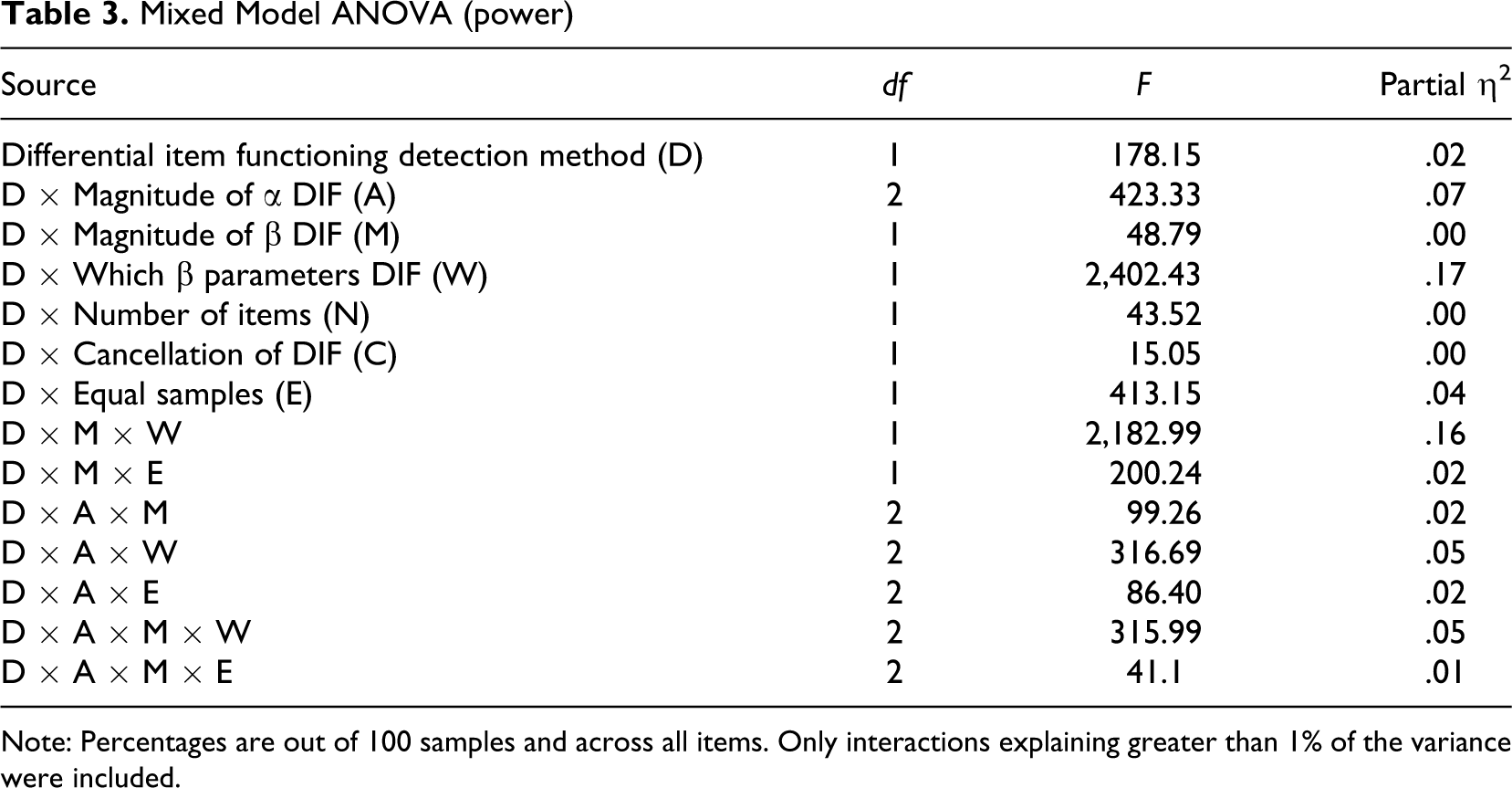
Tables 2 and 3 present effect sizes for the mixed model ANOVAs. We conducted simple effects analyses for two-way interactions with nontrivial effect sizes. As shown in Table 2, the DIF detection method explained 28% of the variance in Type I error rates, with the LRT being associated with lower Type I errors. The interaction between the DIF detection method and sample equality (partial η² = .15) had the next largest effect. The simple effects analyses revealed that sample equality had a larger effect on Type I errors for NCDIF (partial η² = .13) compared with LRT (partial η² = .00). As shown in Figure 1 , the Type I error rates are similar across test type for equal sample sizes. However, when the samples are unequal, the Type I error rates for NCDIF (18%) were much higher than the Type I error rates for LRT (1%). None of the other manipulations had sizable interaction effects on Type I error rates.

Table 2.

Mixed Model ANOVA (Type I)

Source	df	F	Partial η²
Differential item functioning (DIF) detection method	1	4,347.32	.28
DIF Detection Method × Magnitude of α DIF (A)	2	1.72	.00
DIF Detection Method × Magnitude of β DIF (M)	1	6.30	.00
DIF Detection Method × Which β Parameters DIF (W)	1	0.48	.00
DIF Detection Method × Number of Items (N)	1	38.39	.00
DIF Detection Method × Cancellation of DIF (C)	1	0.13	.00
DIF Detection Method × Equal Samples (E)	1	1,953.44	.15

Note: Percentages are out of 100 samples and across all items. Only interactions explaining greater than 1% of the variance were included.

Table 3.

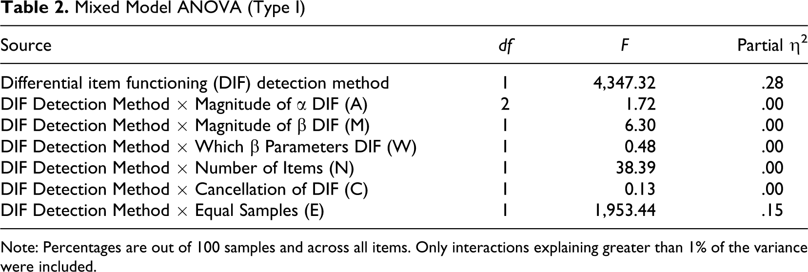
Mixed Model ANOVA (power)

Source	df	F	Partial η²
Differential item functioning detection method (D)	1	178.15	.02
D × Magnitude of α DIF (A)	2	423.33	.07
D × Magnitude of β DIF (M)	1	48.79	.00
D × Which β parameters DIF (W)	1	2,402.43	.17
D × Number of items (N)	1	43.52	.00
D × Cancellation of DIF (C)	1	15.05	.00
D × Equal samples (E)	1	413.15	.04
D × M × W	1	2,182.99	.16
D × M × E	1	200.24	.02
D × A × M	2	99.26	.02
D × A × W	2	316.69	.05
D × A × E	2	86.40	.02
D × A × M × W	2	315.99	.05
D × A × M × E	2	41.1	.01

Note: Percentages are out of 100 samples and across all items. Only interactions explaining greater than 1% of the variance were included.

Figure 1.

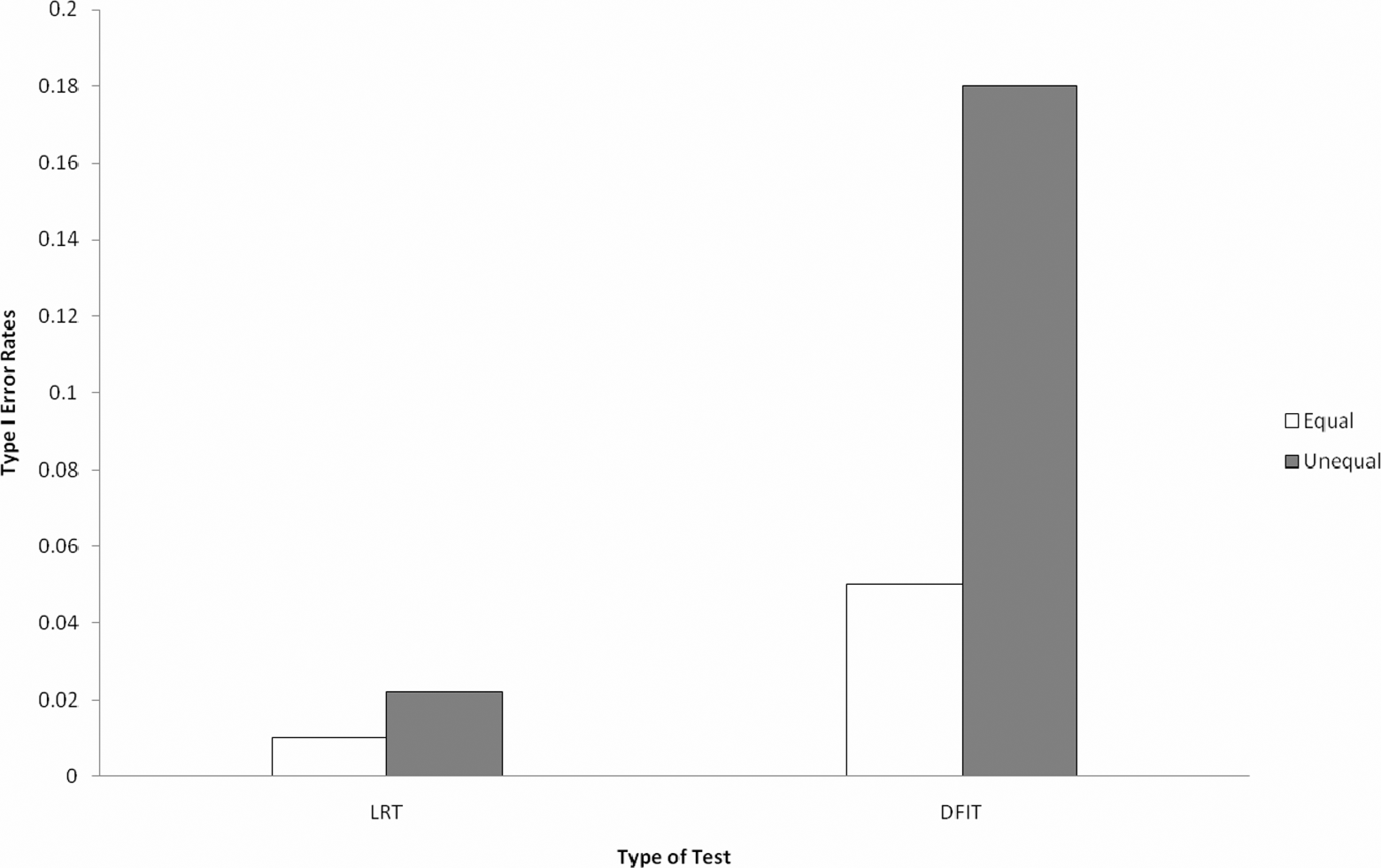
The interaction between the DIF detection method and sample equality.

As shown in Table 3, the DIF detection method explained 2% of the variance in power, with the LRT being associated with higher power. The interaction between DIF detection method and magnitude of α DIF was 7%. Simple effects analyses revealed that the α DIF manipulation had a smaller effect on the power of NCDIF (partial η² = .12) than on the power of LRT (partial η² = .38). The effect size for the interaction between DIF detection method and magnitude of β DIF was smaller (partial η² = .00). The interaction between the DIF detection method and which β parameters were manipulated (partial η² = .17) had the largest effect. The effect was weaker for the NCDIF (partial η² = .06) than for the LRT (partial η² = .15). Similarly, the three-way interaction between DIF detection method, magnitude of β DIF, and which β parameters were manipulated had a large effect (partial η² = .16). The NCDIF does a better job of detecting the DIF when the last two β parameters were changed by 0.40. In contrast, the LRT does a better job of detecting the DIF when the two most extreme β parameters were manipulated changed by 0.40. Few differences were observed when the β parameters were changed by 1.0. The interactions between the number of items (partial η² = .00), cancellation of DIF (partial η² = .00), and sample equality (partial η² = .04) with test type did not explain much variance in power.

Type I Error Rates and Power Estimates

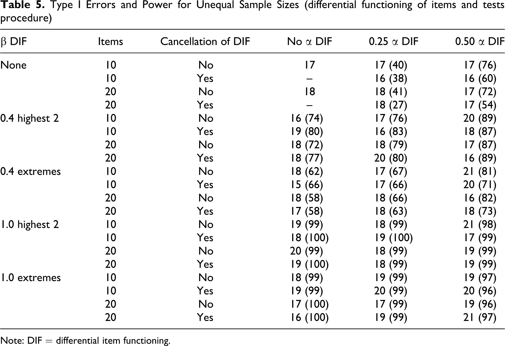
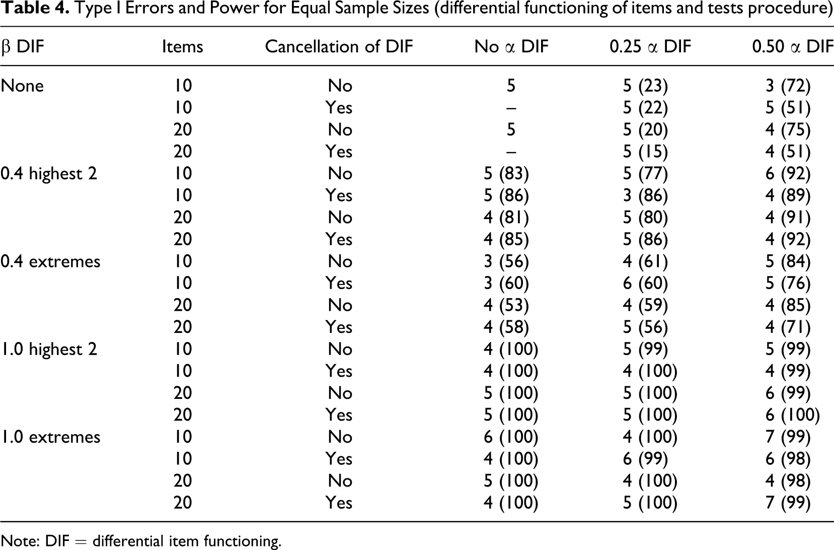
Tables 4 and 5 present the Type I error rates and power estimates for the NCDIF index for equal and unequal sample sizes, respectively. Type I error rates were the percentage of non-DF items that were detected as DF averaged across all 100 samples for each condition. The number in parentheses, power, refers to the number of times the index correctly identified a DF item as DIF per 100 cases. All Type I error rates were less than 7% in the equal samples sizes condition for the NCDIF index. Type I error rates for the unequal sample sizes condition were all between 16% and 21%. Overall, for equal sample sizes, the NCDIF index had acceptable Type I error rates (≤5) in 49 of the 58 conditions but did not have acceptable error rates in any of the conditions for unequal sample sizes.

Table 4.

Type I Errors and Power for Equal Sample Sizes (differential functioning of items and tests procedure)

β DIF	Items	Cancellation of DIF	No α DIF	0.25 α DIF	0.50 α DIF
None	10	No	5	5 (23)	3 (72)
	10	Yes	–	5 (22)	5 (51)
	20	No	5	5 (20)	4 (75)
	20	Yes	–	5 (15)	4 (51)
0.4 highest 2	10	No	5 (83)	5 (77)	6 (92)
	10	Yes	5 (86)	3 (86)	4 (89)
	20	No	4 (81)	5 (80)	4 (91)
	20	Yes	4 (85)	5 (86)	4 (92)
0.4 extremes	10	No	3 (56)	4 (61)	5 (84)
	10	Yes	3 (60)	6 (60)	5 (76)
	20	No	4 (53)	4 (59)	4 (85)
	20	Yes	4 (58)	5 (56)	4 (71)
1.0 highest 2	10	No	4 (100)	5 (99)	5 (99)
	10	Yes	4 (100)	4 (100)	4 (99)
	20	No	5 (100)	5 (100)	6 (99)
	20	Yes	5 (100)	5 (100)	6 (100)
1.0 extremes	10	No	6 (100)	4 (100)	7 (99)
	10	Yes	4 (100)	6 (99)	6 (98)
	20	No	5 (100)	4 (100)	4 (98)
	20	Yes	4 (100)	5 (100)	7 (99)

Note: DIF = differential item functioning.

Table 5.

Type I Errors and Power for Unequal Sample Sizes (differential functioning of items and tests procedure)

β DIF	Items	Cancellation of DIF	No α DIF	0.25 α DIF	0.50 α DIF
None	10	No	17	17 (40)	17 (76)
	10	Yes	–	16 (38)	16 (60)
	20	No	18	18 (41)	17 (72)
	20	Yes	–	18 (27)	17 (54)
0.4 highest 2	10	No	16 (74)	17 (76)	20 (89)
	10	Yes	19 (80)	16 (83)	18 (87)
	20	No	18 (72)	18 (79)	17 (87)
	20	Yes	18 (77)	20 (80)	16 (89)
0.4 extremes	10	No	18 (62)	17 (67)	21 (81)
	10	Yes	15 (66)	17 (66)	20 (71)
	20	No	18 (58)	18 (66)	16 (82)
	20	Yes	17 (58)	18 (63)	18 (73)
1.0 highest 2	10	No	19 (99)	18 (99)	21 (98)
	10	Yes	18 (100)	19 (100)	17 (99)
	20	No	20 (99)	18 (99)	19 (99)
	20	Yes	19 (100)	18 (99)	19 (99)
1.0 extremes	10	No	18 (99)	19 (99)	19 (97)
	10	Yes	19 (99)	20 (99)	20 (96)
	20	No	17 (100)	17 (99)	19 (96)
	20	Yes	16 (100)	19 (99)	21 (97)

Note: DIF = differential item functioning.

Overall, out of the 112 conditions the NCDIF index had acceptable power levels (≥80%) in 70 of the conditions. Acceptable levels of power for the NCDIF index were not found when only the α parameter was manipulated in either condition. Similarly, acceptable power levels were not found when the last two β parameters were changed by 0.40 in either condition. Power levels near 100% were found when the β parameters were changed by 1.00, for both conditions where β parameters were manipulated. Combining α and β DIF generally produced acceptable levels of power, with the exception of when the α parameter was changed by 0.25 and the extreme β parameters where changed by 0.40.

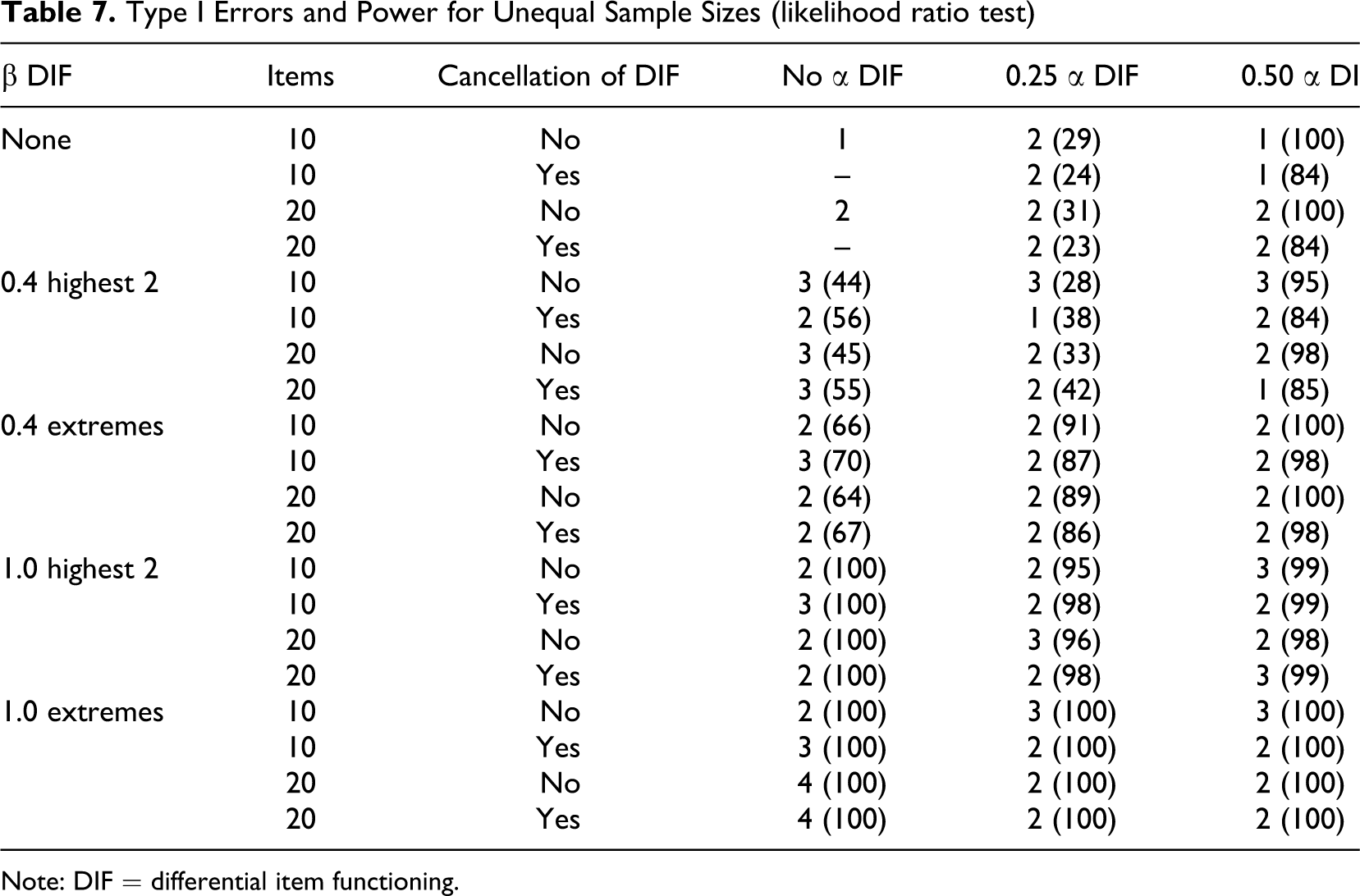
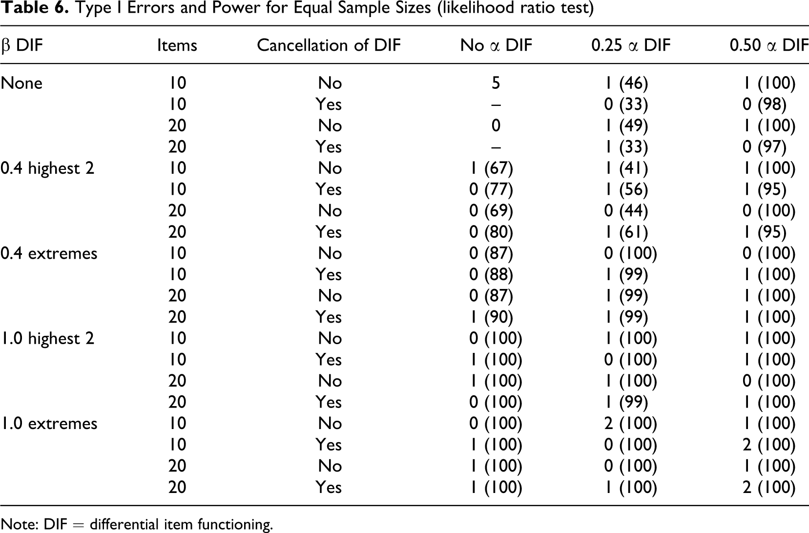
Tables 6 and 7 present the Type I error rates and power estimates for the LRT index for equal and unequal sample sizes, respectively. All Type I error rates were less than 5% across both sample size conditions. Overall, the LRT had acceptable Type I error rates in every condition.

Table 6.

Type I Errors and Power for Equal Sample Sizes (likelihood ratio test)

β DIF	Items	Cancellation of DIF	No α DIF	0.25 α DIF	0.50 α DIF
None	10	No	5	1 (46)	1 (100)
	10	Yes	–	0 (33)	0 (98)
	20	No	0	1 (49)	1 (100)
	20	Yes	–	1 (33)	0 (97)
0.4 highest 2	10	No	1 (67)	1 (41)	1 (100)
	10	Yes	0 (77)	1 (56)	1 (95)
	20	No	0 (69)	0 (44)	0 (100)
	20	Yes	0 (80)	1 (61)	1 (95)
0.4 extremes	10	No	0 (87)	0 (100)	0 (100)
	10	Yes	0 (88)	1 (99)	1 (100)
	20	No	0 (87)	1 (99)	1 (100)
	20	Yes	1 (90)	1 (99)	1 (100)
1.0 highest 2	10	No	0 (100)	1 (100)	1 (100)
	10	Yes	1 (100)	0 (100)	1 (100)
	20	No	1 (100)	1 (100)	0 (100)
	20	Yes	0 (100)	1 (99)	1 (100)
1.0 extremes	10	No	0 (100)	2 (100)	1 (100)
	10	Yes	1 (100)	0 (100)	2 (100)
	20	No	1 (100)	0 (100)	1 (100)
	20	Yes	1 (100)	1 (100)	2 (100)

Note: DIF = differential item functioning.

Table 7.

Type I Errors and Power for Unequal Sample Sizes (likelihood ratio test)

β DIF	Items	Cancellation of DIF	No α DIF	0.25 α DIF	0.50 α DI
None	10	No	1	2 (29)	1 (100)
	10	Yes	–	2 (24)	1 (84)
	20	No	2	2 (31)	2 (100)
	20	Yes	–	2 (23)	2 (84)
0.4 highest 2	10	No	3 (44)	3 (28)	3 (95)
	10	Yes	2 (56)	1 (38)	2 (84)
	20	No	3 (45)	2 (33)	2 (98)
	20	Yes	3 (55)	2 (42)	1 (85)
0.4 extremes	10	No	2 (66)	2 (91)	2 (100)
	10	Yes	3 (70)	2 (87)	2 (98)
	20	No	2 (64)	2 (89)	2 (100)
	20	Yes	2 (67)	2 (86)	2 (98)
1.0 highest 2	10	No	2 (100)	2 (95)	3 (99)
	10	Yes	3 (100)	2 (98)	2 (99)
	20	No	2 (100)	3 (96)	2 (98)
	20	Yes	2 (100)	2 (98)	3 (99)
1.0 extremes	10	No	2 (100)	3 (100)	3 (100)
	10	Yes	3 (100)	2 (100)	2 (100)
	20	No	4 (100)	2 (100)	2 (100)
	20	Yes	4 (100)	2 (100)	2 (100)

Note: DIF = differential item functioning.

The LRT had acceptable power levels in 85 of the conditions. Acceptable levels of power were not found when only the α parameter was changed by 0.25 in either condition. Unlike the NCDIF index, acceptable power was found when only the α parameter was changed by 0.50 in 7 out of the 8 conditions. Acceptable power levels were also found in all conditions in which the two extreme β parameters were changed by 0.4 and the α parameter was changed by at least 0.25. In the unequal sample size condition when there was no α parameter DIF and the β parameter was changed by 0.40, acceptable power was not found. In the equal sample size condition, when there was no α parameter DIF and the extreme two β parameters were changed by 0.40, acceptable power was found in all of the conditions. However, when there was no α parameter DIF and the highest two β parameters were changed by 0.40, acceptable power was found in only one of the conditions. Power was also low when the highest two β parameters were changed by 0.4 and there was α parameter DIF of 0.25.

Additional Analyses

We conducted some exploratory analyses to further examine the Type I error rates for the NCDIF index with unequal sample sizes. One possibility is that the small sample size (N = 250) for the focal group caused the poor Type I error rates. To assess this, we conducted analyses with sample sizes of 500 in the focal group and 1,000 in the reference group using the methods described above. No DIF was manipulated. The Type I error rates were 13% for the 10-item condition and 4% for the 20-item condition. This suggests that larger samples sizes and numbers of items may ameliorate the problem of unequal sample sizes. To further assess the 10-item condition, we conducted analyses to assess whether it was sample size inequality that drove the higher Type I errors for DFIT or whether it was solely the sample size of the focal group. We conducted analyses with sample sizes of 750 in the focal group and 1,000 in the reference group, a condition with 750 in the focal group and 1,500 in the reference group, and also a condition with 750 in the focal group and 3,000 in the reference group. Again, no DIF was manipulated. The Type I error rates were 1% in all three conditions. These results suggest that it is not necessarily the inequality of the sample sizes that creates larger Type I errors but instead the size of the focal group sample.

Discussion

Our first research question concerned how the manipulations affected the Type I error rates across tests. Overall, the LRT resulted in fewer Type I errors compared with NCDIF. In addition, the interaction between test type and sample equality suggested that the LRT had acceptable Type I error rates when sample sizes were equal or unequal. The NCDIF index performed adequately when sample sizes were equal but resulted in too many Type I errors when sample sizes were unequal. None of the other manipulations explained considerable, or greater than 1%, variance in Type I errors. This suggests that for both NCDIF and LRT, the test for items without DIF are not affected by the presence of items with DIF in the test. This is similar to Meade et al.’s (2007) work in which they found acceptable Type I error rates for non-DIF items when there were DIF items on the test.

Our second research question concerned how the manipulations affected the power estimates across tests. Overall, the LRT resulted in greater power to detect α parameter DIF compared with NCDIF. The power estimates suggest that when there was a small change in the α parameter, one test was not better at detecting the DIF than the other test. However, when there was a large change in the α parameter, the LRT had more power than NCDIF did. This suggests that NCDIF does not have the power to detect DIF when the item is more discriminating for one group versus another group. LRT, on the other hand, had acceptable power in all conditions when just the α parameter was changed by a large amount. This indicates that when an item is more discriminating for one group, the LRT is better at detecting this difference. This is consistent with Meade et al.’s (2007) study; they found that the NCDIF index did not consistently detect DIF when there was a small change in α parameter DIF.

Overall, the LRT exhibited greater power to detect β parameter DIF than NCDIF did. However, the interaction between test type and which β parameters DIF suggested that the NCDIF index was better able to detect the DIF when the last two β parameters were manipulated. The LRT was better able to detect the DIF caused by manipulating the two most extreme β parameters. This may have implications for researchers who expect that group differences occur only at the higher end of the scale. For example, applicants who fake may be more likely than incumbents to endorse the higher response options. In this situation, the NCDIF index may more applicable because it is more sensitive to this type of DIF. None of the other manipulations explained considerable variance in power.

Our results suggest that the NCDIF and LRT both had acceptable Type I error rates when sample sizes were equal but that NCDIF produced too many Type I errors when sample sizes were unequal. This was probably caused by the smaller sample sizes used for the focal group. This effect was decreased when the focal group’s sample size increased. The differences in sample sizes between the focal and reference groups did not appear to affect Type I errors.

Finally, the LRT demonstrated more power across conditions. In particular, LRT had greater power to detect DIF caused by different α parameters. This is important because previous research has suggested that NCDIF is not sensitive to this type of DIF (Meade et al., 2007). The LRT also demonstrated acceptable power to detect β DIF in most conditions. However, the NCDIF index has higher power when the last two β parameters are manipulated, but LRT has higher power when the two most extreme β parameters are manipulated. This makes sense because the NCDIF is based on the difference between expected scores for each of the two groups. Changing the two highest β parameters will have a larger effect on expected scores compared to changing the two extreme β parameters.

It is interesting to compare the results of the NCDIF analysis with those of Meade et al. (2007). Similar to Meade et al., we found that the Type I error rates for the NCDIF index were acceptable across most conditions for equal sample sizes and that the NCDIF index is not sensitive to α parameter DIF when there is no β parameter DIF. Meade et al. found that when DIF cancelled, the NCDIF index was better able to detect it. We found this to be the case as well. Finally, similar to Meade et al., we found that NCDIF was more powerful when the last two β parameters had DIF as opposed to the extreme β parameters. However, we found the magnitude of the β DIF had a less of an impact on power than Meade et al. found. This may be due to the fact that, unlike Meade et al., we did not use the condition of changing all four β parameters.

It is more difficult to compare the results for the LRT to previous research because there have been few studies examining it as we did. In general, the previous research has suggested that the LRT has acceptable Type I errors across most situations, and it is powerful when sample sizes are adequate (e.g., Ankenmann et al., 1999; Kim & Cohen, 1998; Meade & Lautenschlager, 2004). Our results are consistent with this. In addition, we found that it compared favorably to the NCDIF index in terms of Type I errors and power.

It is also worthy of note that there is a difference in the number of anchor items across the two methods. The LRT linked on three items, whereas all available non-DIF items were used for linking for the NCDIF. Past researchers have found that increasing the number of anchor items improves DIF detection (e.g., Rivas et al., 2009; Wang & Yeh, 2003). Thus, the NCDIF may have had an advantage over the LRT in our study. However, we found the LRT to be more powerful in general, and our results may provide somewhat of a conservative estimate of the advantage of LRT over NCDIF.

Limitations and Future Research

We investigated only how well NCDIF and LRT could detect DIF when using the GRM as the generating model, but researchers should investigate other models. Generating the data using the generalized partial credit model (Muraki, 1992) or the generalized graded unfolding model (Roberts, Donoghue, & Laughlin, 2000), for example, could have different results. In addition, we generated all of the θ values using a standard normal distribution. Future research could examine the effects of other distributions of θ. It may also be interesting to generate θ values with different distributions for the focal and reference group. For example, it may be useful to assess the performance of tests for DIF when one of the groups has a restricted θ distribution. This may reflect a common situation in comparing applicants and incumbents where one of the groups may have a restricted range.

Researchers should examine different sample sizes and test lengths to ensure that the results from this study are constant across conditions. Using smaller sample sizes that are more likely to occur in the real world would yield useful information. Previous research has found that the LRT does not have optimal power in conditions where sample sizes are less than 500 (e.g., Ankenmann et al., 1999; Meade & Lautenschlager, 2004). More research should examine how the NCDIF handles smaller sample sizes. Finally, there are a number of other DIF detection indices that should be examined in addition to LRT and DFIT. The poly-SIBTEST (Chang, Mazzeo, & Roussos, 1996) and Mantel-Haenszel (Mantel & Haenszel, 1959) are two examples that could be more closely examined and directly compared with the two indices in the present study.

Implications and Recommendations

Our results have several implications for using tests of DIF. First, the LRT should be preferred when there are unequal sample sizes. We found that when the sample sizes are unequal the NCDIF index commits more Type I errors than the LRT and that the LRT still had acceptable Type I errors. This is important because it is likely that DIF studies will have unequal sample sizes. In addition, the LRT has higher power estimates than NCDIF does when sample sizes are unequal.

The LRT has better power across most conditions. In particular, LRT had more power to detect DIF caused by different item discrimination parameters. However, the LRT had less power than NCDIF to detect DIF when the two highest difficulty values were changed by a moderate amount. This suggests that the LRT and NCDIF indices may be able to capture different patterns of DIF, and the preference of which test to use depends on the type of DIF present. In practice, researchers will not know what type of DIF, but they may have some expectations. For example, it may be that applicants are more likely than incumbents to endorse the highest two response options on conscientiousness items. Our findings suggest that the NCDIF index would be better able to detect this and therefore might be preferred for that situation.

Although there are some specific situations where the NCDIF index may be preferred, we suggest that the LRT should be preferred overall because of its consistent Type I error rates and overall power. In addition, we found the LRT is easier to implement than the NCDIF index. The LRT output indicates the χ² statistic associated with the overall item as well as the χ² statistic associated with the α parameter and the β parameter. This allows the researchers to identify where the DIF is located for a particular item. In addition, the LRT does not require the linking or calculation of empirical cutoffs needed by the NCDIF index.

Despite all of the differences mentioned throughout the article, as one reviewer pointed out, it should be noted that NCDIF and LRT are similar methodologies. They are essentially both area methods. The difference lies in how these indices use the area information. NCDIF uses the equated parameter estimates to assess differences between IRFs. The LRT directly calculates the likelihood under the constraint of equal item parameters and compares it against the likelihood if parameters were free. Conceptually, both indices are comparing IRFs. Furthermore, the two indices lead to the same conclusion most of the time.

One issue in using the LRT (and for NCDIF) is choosing the appropriate anchor items. Using anchor items that exhibit DIF can lead to inflated Type I errors. In the present study, we had the advantage of knowing a priori which items had DIF. Obviously, this would not be the case in most situations. This creates a bit of a chicken-and-egg problem where researchers need to identify a couple of items that do not have DIF that can serve as anchors to test for DIF. Past researchers have recommended using an initial run of the constrained baseline method to identify DIF-free items that can serve as anchors (Stark et al., 2006). The major problem with the constrained baseline method is the large Type I errors. Thus, items that are not flagged as having DIF with this method probably do not have DIF. This approach is somewhat similar to the multistage linking process, often called iterative linking, required by the NCDIF index (Candell & Drasgow, 1998), and will likely lead to the identification of appropriate anchor items.

Footnotes

The author(s) declared no potential conflicts of interest with respect to the authorship and/or publication of this article.

The author(s) received no financial support for the research and/or authorship of this article.

References

Angoff

W. H.

Ford

S. F.

(1973) Item-race interaction on a test of scholastic aptitude Journal of Educational Measurement 10 doi:10.1111/j.1745-3984.1973.tb00787.x

Ankenmann

R. D.

Witt

E. A.

Dunbar

S. B.

(1999) An investigation of the power of the likelihood ratio goodness-of-fit statistic in detecting differential item functioning Journal of Educational Measurement 36 doi:10.1111/j.1745-3984.1999.tb00558.x

Baker

F. B.

(1995). EQUATE 2.1: Computer program for equating two metrics in item response theory [Computer program]. Madison: University of Wisconsin, Laboratory of Experimental Design

Bolt

D. M.

(2002) A Monte Carlo comparison of parametric and nonparametric polytomous DIF detection methods Applied Measurement in Education 15 doi:10.1207/S15324818AME1502_01

Braddy

P. W.

Meade

A. W.

Johnson

E. C.

(2006). Practical implications of using different tests of measurement invariance for polytomous measures. Paper presented at the 21st Annual Conference of the Society for Industrial and Organizational Psychology, Dallas, TX.

Candell

G. L.

Drasgow

(1988) An iterative procedure for linking metrics and assessing item bias in item response theory Applied Psychological Measurement 12

Chang

H. H.

Mazzeo

Roussos

(1996) Detecting DIF for polytomously scored items: An adaptation of the SIBTEST procedure Journal of Educational Measurement 33

Collins

W. C.

Raju

N. S.

Edwards

J. E.

(2000) Assessing differential functioning in a satisfaction scale Journal of Applied Psychology 85 doi:10.1037/0021-9010.85.3.451

Donovan

M. A.

Drasgow

Probst

T. M.

(2000) Does computerizing paper-and-pencil job attitude scales make a difference? New IRT analyses offer insight Journal of Applied Psychology 85 doi:10.1037/0021-9010.85.2.305

10.

Flowers

C. P.

Oshima

T. C.

Raju

N. S.

(1999) A description and demonstration of the polytomous-DFIT framework Applied Psychological Measurement 23 doi:10.1177/01466219922031437

11.

Henry

M. S.

Raju

N. S.

(2006) The effects of trailed and situational impression management on a personality test: An empirical analysis Psychological Science 48

12.

Holland

P. W.

Thayer

D. T.

(1988) Differential item functioning and the Mantel-Haenszel procedure Wainer

Braun

H. I.

(Eds.), Hillsdale, NJ

Lawrence Erlbaum

13.

Kim

S. -H.

Cohen

A. S.

(1988) Detection of differential item functioning under the graded response model with the likelihood ratio test Applied Psychological Measurement 22 doi:10.1177/014662169802200403

14.

Lord

F. M.

(1980) Applications of item response theory to practical testing problems. Hillsdale, NJ

Lawrence Erlbaum

15.

Mantel

Haenszel

(1959) Statistical aspects of the analysis of data from retrospective studies of disease Journal of the National Cancer Institute 22

16.

Maurer

T. J.

Raju

N. S.

Collins

W. C.

(1998) Peer and subordinate performance appraisal measurement equivalence Journal of Applied Psychology 83

17.

Meade

A. W.

(2010) A taxonomy of effect size measures for the differential functioning of items and scales Journal of Applied Psychology 95

18.

Meade

A. W.

Lautenschlager

G. J.

(2004) A comparison of item response theory and confirmatory factor analytic methodologies for establishing measurement equivalence/invariance Organizational Research Methods 7 doi:10.1177/1094428104268027

19.

Meade

A. W.

Lautenschlager

G. J.

Johnson

E. C.

(2007) A Monte Carlo examination of the sensitivity of the differential functioning of items and tests framework for tests of measurement invariance with Likert data Applied Psychological Measurement 31 doi:10.1177/0146621606297316

20.

Morales

L. S.

Flowers

Gutierrez

Kleinman

Teresi

J. A.

(2006) Item and scale differential functioning of the Mini-Mental State Exam assessed using the differential item and test functioning (DFIT) framework Medical Care 44

21.

Morris

(2008). Polycov [Computer program]. Retrieved August 2009 from http://mypages.iit.edu/~morriss/polycov/polycov.html

22.

Muraki

(1992) A generalized partial credit model: Application of an EM algorithm Applied Psychological Measurement 16 doi:10.1177/014662169201600206

23.

Muraki

Bock

R. D.

(2003). PARSCALE 4: IRT item analysis and test scoring for rating-scale data [Computer program]. Chicago: Scientific Software

24.

Oshima

T. C.

Kushubar

Scott

J. C.

Raju

N. S.

(2009) St. Paul, MN

Assessment Systems Corporation

25.

Oshima

T. C.

Raju

N. S.

Nanda

A. O.

(2006) A new method for assessing the statistical significance in the differential functioning of items and tests (DFIT) framework Journal of Educational Measurement 43 doi:10.1111/j.1745-3984.2006.00001.x

26.

Raju

N. S.

(1988) The area between two item characteristic curves Psychometrika 53 doi:10.1007/BF02294403

27.

Raju

N. S.

(1990) Determining the significance of estimated signed and unsigned areas between two item response functions Applied Psychological Measurement 14 doi:10.1177/014662169001400208

28.

Raju

N. S.

Fortmann-Johnson

K. A.

Kim

Morris

S. B.

Nering

M. L.

Oshima

T. C.

(2009) The item parameter replication method for detecting differential functioning in the polytomous DFIT framework Applied Psychological Measurement 33

29.

Raju

N. S.

Laffitte

L. J.

Byrne

B. M.

(2002) Measurement equivalence: A comparison of methods based on confirmatory factor analysis and item response theory Journal of Applied Psychology 87 doi:10.1037/0021-9010.87.3.517

30.

Raju

N. S.

van der Linden

W. J.

Fleer

P. F.

(1995) IRT-based internal measures of differential functioning of items and tests Applied Psychological Measurement 19 doi:10.1177/014662169501900405

31.

Rivas

G. E.

Stark

Chernyshenko

O. S.

(2009) The effects of referent item parameters on differential item functioning detection using the free baseline likelihood ratio test Applied Psychological Measurement 33 doi:10.1177/0146621608321760

32.

Roberts

J. S.

Donoghue

J. R.

Laughlin

J. E.

(2000) A general item response theory model for unfolding unidimensional polytomous responses Applied Psychological Measurement 24 doi:10.1177/01466216000241001

33.

Robie

Zickar

M. J. , & Schmit, M. J.

(2001) Measurement equivalence between applicant and incumbent groups: An IRT analysis of personality scales Human Performance 14 doi:10.1207/S15327043HUP1402_04

34.

Samejima

(1969). Estimation of latent ability using a response pattern of graded scores. (Psychometric Monograph No. 17). Richmond, VA: Psychometric Society

35.

Stark

Chernyshenko

O. S.

Drasgow

Williams

B. A.

(2006) Detecting differential item functioning with confirmatory factor analysis and item response theory: Toward a unified strategy Journal of Applied Psychology 91 . doi:10.1037/0021-9010.91.6.1292

36.

Thissen

(2001). IRTLRDIF v.2.0b: Software for the computation of the statistics involved in item response theory likelihood-ratio tests for differential item functioning [Computer software]. Chapel Hill: University of North Carolina.

37.

Thissen

Steinberg

Wainer

(1988) Use of item response theory in the study of group differences in trace lines Wainer

Braun

H. I.

(Eds.), Hillsdale, NJ

Lawrence Erlbaum

38.

Wang

W. C.

(2004) Effects of anchor item methods on differential item functioning detection within the family of Rasch models Journal of Experimental Education 72

39.

Wang

W. C.

Yeh

Y. L.

(2003) Effects of anchor item methods on differential item functioning detection with the likelihood ratio test Applied Psychological Measurement 27 doi:10.1177/0146621603259902