Methodological Advances in the Analysis of Bipartite Networks

Abstract

Network-based research in the management field largely assumes one-mode (unipartite) networks, despite the widespread presence of two-mode (bipartite) networks. In empirical work, scholars usually project a bipartite network onto a unipartite network, ignoring issues related to the interdependence of ties and potential loss of information. Yet new advances in measures and methods related to bipartite networks in the fields of sociology, physics, and biology may make such tactics unnecessary. This article presents an overview of three research streams related to bipartite networks, namely, (a) refinements related to the projections of bipartite networks onto unipartite networks; (b) the extension of networks measures from unipartite networks to bipartite networks, with a focus on clustering coefficients; and (c) approaches unique to bipartite networks, such as nestedness. We apply these approaches and compare the findings of a traditional unipartite network analysis using both a simple example and a sample of 10,223 directors of 1,528 Indian firms in 2009.

Keywords

bipartite networks weighted networks small world clustering coefficient nestedness

In the past decade, studies of social network analysis have expanded notably (Borgatti & Halgin, 2011), mostly in the form of studies of one-mode (unipartite) networks. In a unipartite network, the nodes are all of one type (e.g., individuals, firms), and ties link only these same types of nodes. Popular examples include friendship networks at the individual level or alliance networks at the firm level. Yet a considerable number of networks actually are two-mode (or bipartite or affiliation) networks, featuring ties between two different types of nodes, such as board networks (Davis, Yoo, & Baker, 2003), specialists involved in television productions (Zaheer & Soda, 2009), authors of team-authored research papers (Newman, 2001), firms as members of multiparty alliances (Greve, Baum, Mitsuhashi, & Rowley, 2010), and countries involved in product trade (Schweitzer et al., 2009).

Perhaps because of the lack of appropriate measures and methods to address these bipartite networks (Latapy, Magnien, & Vecchio, 2008; Wasserman and Faust, 1994), most empirical work projects bipartite networks onto unipartite networks. However, this approach creates issues involving information loss and tie interdependence (Conaldi, Lomi, & Tonellato, 2012). Furthermore, characteristics for affiliations are indirectly constructed via network attributes of their members rather than the affiliations’ network characteristics (e.g., Zaheer & Soda, 2009). The relevant concerns are relatively common, in that researchers often encounter either latent bipartite network structures, such as in the case of niche overlaps across resource complementarities (Chung, Singh, & Lee, 2000) or mutual forbearance (Lomi & Pallotti, 2012), or deliberately choose a unipartite network representation.

In the network analysis field, bipartite approaches trail unipartite views, yet in other areas, such as sociology, physics, and biology, we find significant advances in bipartite network analyses. We therefore recommend an excursion for management scholars, such that we look to other realms to discover the latest advances in network analysis (Dionne et al., 2012) in addition to those in the management literature with bipartite exponential graph models (Wang, Sharpe, Robins, & Pattison, 2009) and stochastic actor-based modeling for bipartite networks (Conaldi et al., 2012). Specifically, we present three streams of research related to bipartite networks. First, we introduce refinements related to projections of bipartite networks onto unipartite networks. Second, we note extensions of network measures from unipartite to bipartite networks, for which the focus is on clustering coefficient, a key measure for small-world characteristics, network cohesion, and embeddedness. Third, we consider approaches unique to bipartite networks. To synthesize these advances, we propose a two-dimensional framework of unipartite versus bipartite approaches and complementary node and network perspectives.

In the following sections, we begin with a simple example to illustrate the limitations of projecting bipartite networks onto unipartite versions. We then discuss some alternative approaches for analyzing bipartite networks and illustrate these approaches on the basis of an application to the director-board network of all publicly listed firms in India in the year 2009.

Bipartite Networks and Projections to Unipartite Networks

Background

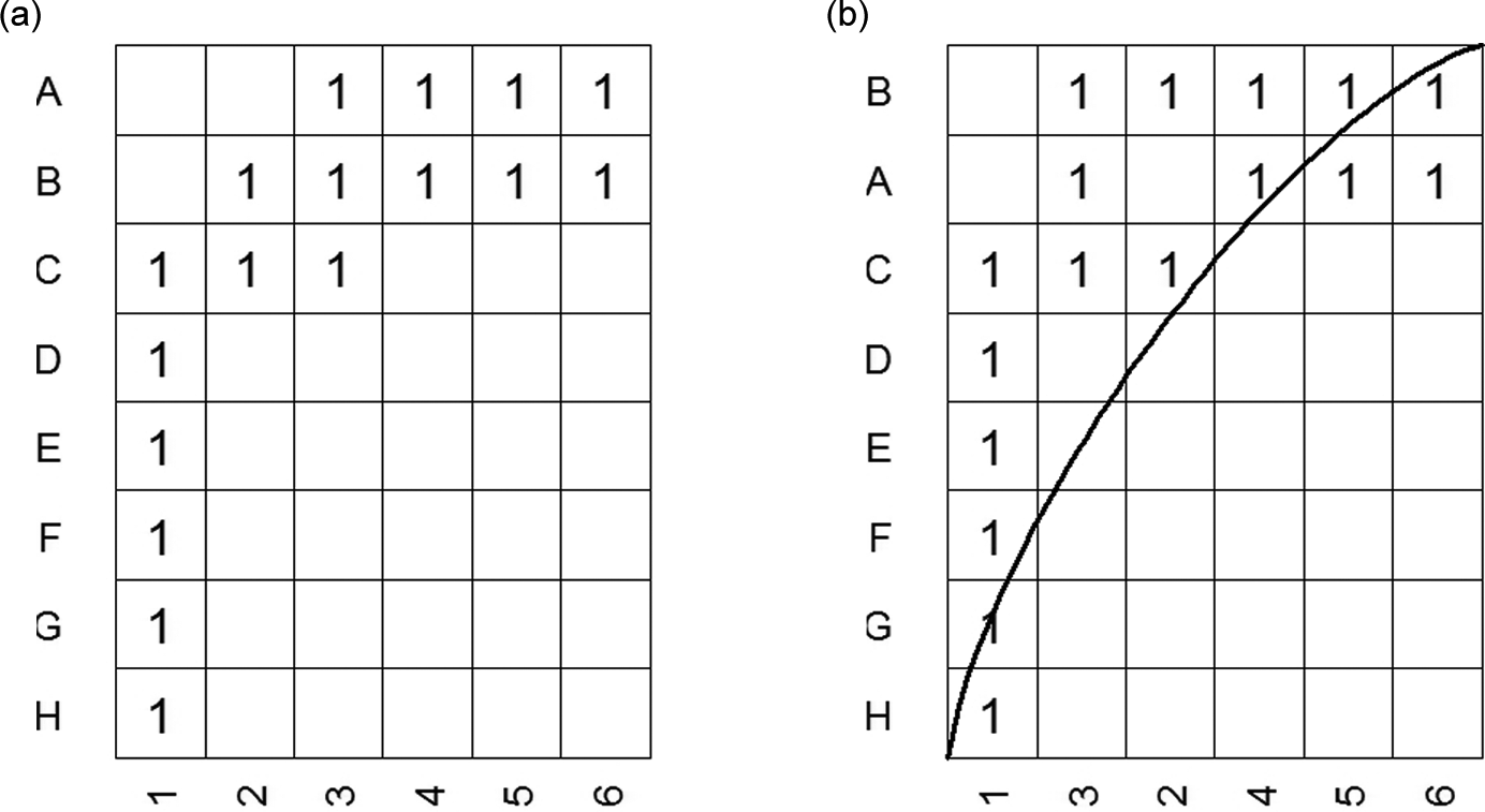
Bipartite networks contain ties between two different types of nodes (Wasserman & Faust, 1994). In many cases, one of the node types is actors; the other might refer to events, such as membership in a group, meeting, corporate board, alliance, the environment, or markets. Such bipartite networks can be described with an incidence matrix (Figure 1a), with elements $a_{i j}$ , in which the N rows (index i) are the actors and the M columns (index j) refer to the events.

Figure 1.

Bipartite network with Actors A to H and events 1 to 6. (a) Original order. (b) Nodes ordered along degree with isocline.

An incidence matrix usually is rectangular, because the number of actors and events does not need to be equal. If an actor participates in an event, the incidence matrix element $a_{i j}$ takes a value greater than 0; otherwise, it is 0. In many cases, the networks appear binary, with values of either 0 or 1. For simplicity, we assume such a structure for this discussion, though some of the methods we introduce are also applicable to weighted bipartite networks.

The two-by-two matrix in Figure 2 refers to the choice of network type (unipartite or bipartite) and the unit of analysis (node level or network level). Most research into bipartite networks appears in Quadrant I, that is, analyses of unipartite networks at the node level. Quadrant II encompasses analyses of unipartite networks at the network level, as reflected initially in the small-world analysis offered by Watts and Strogatz (1998). Since then, similar analyses have been applied to board networks (e.g., Baum, Shipilov, & Rowley, 2003; Davis et al., 2003). Quadrant III refers to analyses of bipartite networks at the node level, for which the analytic tools include centrality measures proposed by Borgatti and Everett (1997) and Faust (1997). These works have spurred research outside of management domain in areas such as ecological networks. Quadrant IV refers to the analysis of bipartite networks at the network level. In this realm, Faust (1997) discusses the structure of bipartite networks with Galois lattices; Battiston and Catanzaro (2004) further analyze distributions of bipartite node characteristics across different networks. However, Quadrant IV lacks network-level measures that capture structural properties of the network.

Figure 2.

Decision matrix for the analysis of bipartite networks.

The choice of a quadrant in the matrix depends on the particular research questions, hypotheses, and data. If the objective is to use node characteristics, such as centrality measures, as explanatory variables in regression analyses, scholars might be interested in either Quadrant I or Quadrant III, depending on whether the network is a projected unipartite or the original bipartite. However, if the objective is to compare different networks, scholars focus on Quadrant II or Quadrant IV, again depending on whether the network is unipartite or bipartite. For each quadrant in Figure 2, we suggest transferring advances in analyses of bipartite networks from other disciplines to management research. We introduce these new methods in greater detail next.

Projections of Bipartite Networks to Unipartite Networks

Researchers often transform bipartite networks into unipartite networks using a projection to connect actors that participate in the same event with one another. The resulting projection for actors results in the unipartite network structure in Figure 3.

Figure 3.

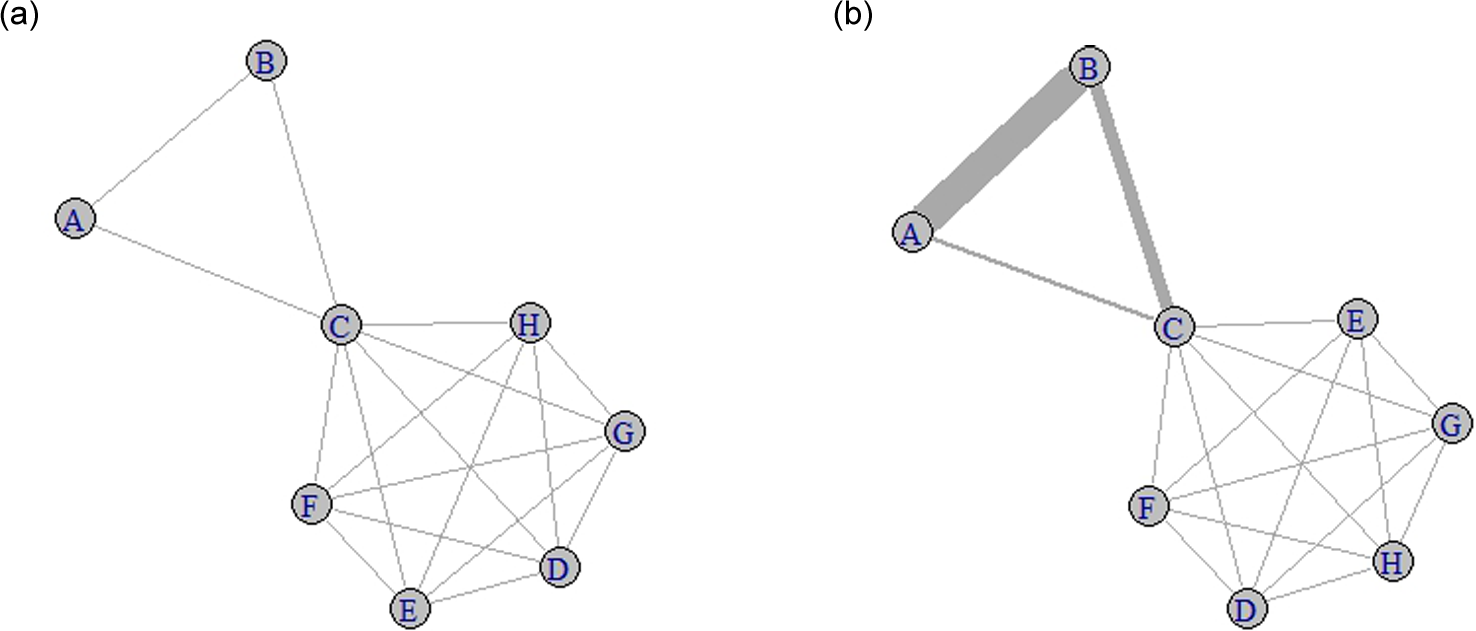
Example unipartite network with eight nodes and ties between them. (a) Binary projection. (b) Weighted projection.

Figure 3a illustrates a simple unipartite network with eight nodes and binary ties. As explained previously, the nodes might stand for employees in a firm, such that the ties between them result from their participation in common events, such as meetings, and lead to conduits for information flows. They can also symbolize firms, tied by their sale of products in the same national markets, such that the ties facilitate information flow or competitive actions. In Figure 3a, we can discern a core of well-connected nodes (C to H) and two peripheral nodes (A and B). Node C has a prominent position, connecting the dense core with the periphery, which allows it to control information flows. Such projections normally result in undirected networks, which is our assumption for the following discussion.

The projection example illustrated by Figure 3a demonstrates some limitations of deriving unipartite networks from bipartite networks. First, the ties between two employees in this example do not indicate the number of meetings they share. Even if such information determines the weight of the tie (Figure 3b), well-known network measures do not take such weights into account. Second, the ties of Nodes C-H are created simultaneously by their participation in the same meeting. However, in this large connected group, employees do not necessarily have personal ties with one another. As the meeting size increases, we obtain a larger group of connected employees, even as the likelihood of mutual interaction among any pair of employees decreases. Third, this approach ignores the possibility that bipartite networks have characteristics unique to their specific nature, which cannot be captured from a unipartite network perspective.

Although this projection can apply to both types of nodes, most researchers focus on the actor-oriented projection. Furthermore, the projected unipartite network is often binary, such that all existing ties appear equally important (weight = 1). However, granting equal weights to different shared events results in information loss. In this example, the binary network in Figure 3a ignores the information that Actors A and B share four events. Assigning weights to the ties equal to the number of co-occurrences can account for this difference, such that the tie between A and B should take a weight of 4, while the others exhibit a weight of 1. A similar weighting approach appears in several studies; for example, Kogut, Urso, and Walker (2007) use the number of deals between two venture capital firms, and Greve et al. (2010) note the number of shared routes between two shipping liners. Weighting by co-occurrence effectively accounts for the number of links, but it ignores the acquaintance of the focal actor with other actors in an affiliated organization.

Newman (2001) argues that in scientific collaboration networks, with researchers as actors and joint publications as events, the number of coauthors matter, such that authors’ interactions with their coauthors should be scaled by 1/(n – 1), where n is the number of coauthors. In the case of a two-author collaboration, the focal author interacts solely with the second author; in a case of three authors, the focal author’s interaction is shared between the other two authors. The same logic can apply in our illustration, resulting in a weight of 3.5 for the tie between A and B, 1.5 for the tie between B and C, and 0.2 for all other ties.

Measures of Weighted Unipartite Networks

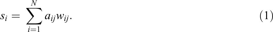
The assignment of weights in the projection thus helps retain important information, but this tactic can be exploited only if methods for weighted networks are available. Here, we discuss extensions of centrality measures and clustering coefficients to weighted networks (Barrat, Barthelémy, Pastor-Satorras, & Vespignani, 2004; Opsahl, Agneessens, & Skvoretz, 2010). We use $w_{i j}$ to denote the weight of the tie between nodes i and j.

Centrality measures

Barrat et al. (2004) extend degree centrality from binary to weighted networks, in the form of strength $s_{i}$ , which is the sum of the weights of the focal node’s ties in a unipartite network:

s_{i} = \sum_{i = 1}^{N} a_{i j} w_{i j} .

This standard, commonly used definition of tie strength (e.g., Lin, Yang, & Irem, 2007) ignores the number of neighbors. For example, Node A, as well as Nodes D through H, have strength of 5 using the weight of co-occurrence, but their degree centrality and position in the network differ widely. The main contribution to A’s strength comes from its strong connection with B, whereas Nodes D through H exhibit weak ties to a rather large number of neighbors. Whereas A may receive more sticky information or tacit knowledge from B, through their repeated interactions, D to H are more likely to receive freely available information from a diverse group of nodes.

Opsahl et al. (2010) instead define centrality measures that take both the weight and the number of ties into consideration and acknowledge the relative importance of strength using a positive tuning parameter α, such that

w e i g h t e d d e g r e e c e n t r a l i t y = k_{i} {(\frac{s_{i}}{k_{i}})}^{α} = k_{i}^{1 - α} s_{i}^{α},

where

k_{i}

is the degree of node i. For α equal to 0, the weighted degree centrality is equivalent to the degree, whereas for α equal to 1, it is equivalent to strength. The larger the value of α, the more important is the weight of the ties and thus the strength of the node.

Table 1 contains the weighted degrees for four values of α. The weighted degrees for Nodes D through H remain unchanged, due to the binary weight of their ties, but those for Nodes A through C change with the tuning parameter and the relative values for all nodes. A low α value may be more suitable if the focus of the research is on the flow of easily available information, such as discussions in a meeting. In contrast, a larger value of α may be more suitable if the research interest pertains to the flow of sensitive information or tacit knowledge that requires a strong tie.

Table 1.

Weighted Degree Centralities for Simple Example Network With Co-Occurrence Weights and Different Values of the Tuning Parameter α.

Node	Degree (alpha = 0)	Weighted degree (alpha = 0.5)	Strength (alpha = 1)	Weighted degree (alpha = 1.5)
A	2	3.16	5	7.9
B	2	3.46	6	10.39
C	7	7.48	8	8.55
D	5	5	5	5
E	5	5	5	5
F	5	5	5	5
G	5	5	5	5
H	5	5	5	5

Both betweenness and closeness centrality measures for two nodes, i and j, reflect the shortest path between the two nodes. For binary networks, it is the number of ties between node i and j. For example, in Figure 3, the shortest path between A and H is 2, through the Paths A-C and C-H. Opsahl et al. (2010) suggest extending both measures, using extensions of the shortest path 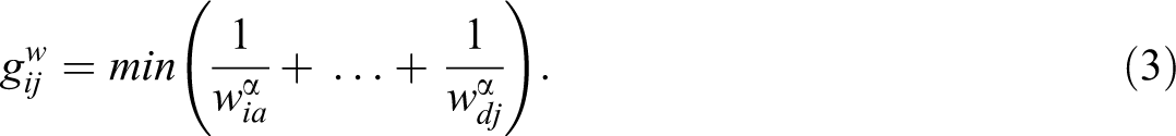$g_{i j}^{w}$ for weighted networks (Brandes, 2001), and taking the weight of ties into account. They also recommend adding a positive tuning parameter α that defines the relative importance of the weight of ties over the number of intermediary nodes on the path:

g_{i j}^{w} = m i n (\frac{1}{w_{i a}^{α}} + \dots + \frac{1}{w_{d j}^{α}}) .

For α equal to 0, $g_{i j}^{w}$ is equivalent to the shortest path for binary networks. For α equal to 1, $g_{i j}^{w}$ is equivalent to the shortest path for weighted networks (Brandes, 2001; Newman, 2001), in which the inverse weight measures the resistance to transmission over the tie. For α less than 1, a few intermediate nodes with weak ties are preferred over a longer path with strong ties. For α greater than 1, the weights of ties gain importance with the number of intermediaries and length, but more strongly connected paths are preferred. Using the weighted shortest path from Equation 3, we can define closeness centrality and betweenness centrality as usual, that is, as the inverse sum of all shortest paths and the ratio of shortest paths through the focal node, respectively.

In our example (Figure 3), the shortest path between A and D through C in the binary case changes to A-B-C-D when α = 1. Despite the additional intermediary node, this path may provide a faster conduit for information because the ties are rather strong. Although C remains the connecting node for the clique of D to H, B also assumes a nonzero betweenness centrality. For example, if the events are firms selling in different national markets, C may be able to gain information on A’s products in the Joint Market/Event 3, but it cannot learn A’s global strategy. However, C may receive some information from B, who observes A in more markets and can infer its strategy accordingly. If this example pertained to employees within a firm, we would suggest that more codified, accessible information can flow through weak ties, and a small α is appropriate, but more complex and tacit information flow is better described with a higher α.

All three extensions of the centrality measures match well-defined measures in binary networks for all weights equal to 1. Their key limitation is the assumption that the weights reflect a ratio scale. Although the exact choice of α is a concern for specifying a certain centrality measure, it also provides an opportunity to distinguish whether the weight of ties or the number of intermediate nodes is important by comparing the results of the unweighted measures with those of the weighted measures.

Clustering coefficient

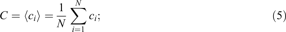
The clustering coefficient measures the cliquishness of the local environments, according to the average local clustering by nodes in their neighborhoods. The neighborhood of node i with 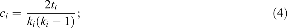$k_{i}$ neighbors has, at a maximum, $k_{i} (k_{i} - 1) / 2$ ties. The local clustering coefficient $c_{i}$ for node i then equals the number of actual ties $t_{i}$ divided by the maximum number of ties (Equation 4), equivalent to the network density of the local network in node i’s neighborhood. The global clustering coefficient C represents the average of the node-specific clustering coefficients over all nodes in the network, such that

c_{i} = \frac{2 t_{i}}{k_{i} (k_{i} - 1)};

C = ⟨ c_{i} ⟩ = \frac{1}{N} \sum_{i = 1}^{N} c_{i};

Such clustering coefficients have been subject to two main refinements in recent literature: corrections for the greater cliquishness of projected bipartite networks (Newman, Strogatz, & Watts, 2001) and accounting for extensions for weighted networks (Barrat et al., 2004; Opsahl & Panzaras, 2009).

The projection of bipartite networks leads to natural clustering of the projected unipartite networks. In our example, attendance at event 1 leads to a clique of six members, all connected with one another. The projected unipartite networks thus are a collection of cliques, connected by actors that join multiple events. Large events in the bipartite network result in large cliques that create a relatively highly clustered network. Newman et al. (2001) provide a comprehensive framework that seeks to generate functions for degree distributions and can account for such clustering; they thus propose the Newman-Strogatz-Watts (NSW) small-world coefficient. Conyon and Muldoon (2006) apply this method to board networks from Germany, the United States, and the United Kingdom and find that none of these networks showed clustering coefficients higher than expected from a bipartite random network with the same degree distribution. In Appendix A, we provide a detailed derivation of the formula to calculate the path length and clustering coefficient, using a given degree distribution for both types of nodes. We also illustrate it in our real example of Indian firms’ board networks.

Barrat et al. (2004) define a weighted clustering coefficient $c_{i}^{w}$ that accounts for different weights, arguing that a stronger tie between nodes leads to greater cohesion than does a weak tie:

c_{i}^{w} = \frac{1}{s_{i} (k_{i} - 1)} \sum_{j, h}^{} \frac{w_{i j} + w_{i h}}{2} a_{i j} a_{i h} a_{j h} .

For each triplet in the neighborhood of the focal node i, the average weight of its ties, rather than the existence of a tie, counts. The sum over all triplets is normalized by the average weight and number of possible triplets, which guarantees that the weighted clustering coefficient falls between 0 and 1. For constant weights, Equation 6 is equivalent to the clustering coefficient defined by Watts and Strogatz (1998). The weighted global clustering coefficient $C^{w}$ is the mean over all individual $c_{i}^{w}$ , and C(k) is the average clustering coefficient of all nodes with degree k.

In our example, the weighted clustering coefficient for the Newman projection for Nodes D-H, with weights of 0.2, is still 1, because all the weights are the same. Therefore, this technique does not resolve the problem of inflated clustering coefficients for small-world analysis.

Bipartite Networks

Bipartite networks entered the organizational field nearly 40 years ago, in a seminal article by Breiger (1974) about the duality of people and groups. Despite this long history and the ubiquity of bipartite networks, analytical methods for assessing bipartite networks still lag behind those of unipartite networks (Wasserman & Faust, 1994). Some prominent efforts to devote more attention to bipartite networks include work by Borgatti and Everett (1997), Faust (1997), and Latapy et al. (2008), as well as the use of bipartite networks in food webs (who eats whom) in an ecological community (see Bascompte & Jordano, 2007). The centrality measures suggested by Borgatti and Everett (1997) are well established; here, we focus on clustering coefficients in bipartite networks, nestedness, and bipartite random networks.

Clustering Coefficients

The primary question for the local clustering coefficient in unipartite networks pertains to closure: To what extent do existing ties of node i to nodes j and k lead to the formation of a tie between the nodes j and k? In bipartite projections though, tie formation is not independent, such that triangles form simultaneously, as demonstrated in Figure 3. Furthermore, the definition of the clustering coefficient (Equation 4) cannot be extended to bipartite networks because the connection of direct neighbors of the same type is prohibited and triangles cannot exist.

Robins and Alexander (2004) introduce a bipartite clustering coefficient as an extension of the unipartite global version, that is, of the global measure based on the number of triangles in the network (often referred to as transitivity). A dual aggregation technique introduced by Breiger and Mohr (2004) acts on quantitative bipartite networks, defining the clustering coefficient for binary networks. Latapy et al. (2008) propose extending the local clustering coefficient to bipartite networks with a more abstract definition of overlapping neighborhoods, according to the directly connected nodes for i and j. The overlap equals the fraction of joint neighbors in both neighborhoods:

o v e r l a p (i, j) = \frac{|N (i) \cap N (j)|}{|N (i) \cup N (j)|},

where the numerator indicates the number of shared neighbors, and the denominator is the number of nodes in the combined neighborhoods. In this example, the neighborhood of Actor B is Events 2 through 6, whereas the neighborhood of Actor C is Events 1, 2, and 3. The overlap between Node B and C thus is the number of joint Events 2 and 3, divided by number of events 1-6, which leads to an overlap of one third. To account for heterogenous event sizes resulting in small clustering coefficients according to Equation 7, we can normalize the values by either the smallest or largest of the two neighborhoods rather than the combined neighborhood:

o v e r l a p (i, j) = \frac{|N (i) \cap N (j)|}{m i n (|N (i)|, |N (j)|)}, o v e r l a p (i, j) = \frac{|N (i) \cap N (j)|}{m a x (|N (i)|, |N (j)|)} .

The bipartite local clustering coefficient for node i equals the average of its nonzero overlaps:

c_{i}^{b i p a r t i t e} = \frac{\sum_{j \in N (i, 2)} o v e r l a p (i, j)}{|N (i, 2)|} .

where

N (i, 2)

is the neighborhood of node i with a distance of 2, such that nodes of the same type are connected by a joint node of the other type. Overlap can reflect any of the three types defined by Equations 7 to 9. For example, in the case of normalization by the minimum, the overlap between B and C is two thirds, whereas normalization by the maximum indicates two fifths. The local bipartite clustering coefficient also can be aggregated to a clustering coefficient for each type of node and for the complete network. In Table 2, we provide node-specific clustering coefficients and their averages for the actors. The weighted clustering coefficient differs only slightly from the binary version for actor C; it is 1 for all other nodes because each node takes an equal weight when only one event is shared. The differences grow more pronounced for projections of larger networks with more joint events, though nodes sharing one event always have a clustering coefficient of 1. The bipartite clustering coefficient also differs more strongly from the binary and weighted unipartite versions, and nodes A, B, and C have different values.

Table 2.

Clustering Coefficients for the Simple Network.

Node	Binary unipartite	Weighted unipartite weight 1 Barrat	Weighted unipartite weight 2 Barrat	Bipartite union	Bipartite minimum	Bipartite maximum
A	1	1	1	0.48	0.67	0.53
B	1	1	1	0.53	0.83	0.6
C	0.52	0.48	0.33	0.3	0.86	0.33
D	1	1	1	0.67	1	0.89
E	1	1	1	0.67	1	0.89
F	1	1	1	0.67	1	0.89
G	1	1	1	0.67	1	0.89
H	1	1	1	0.67	1	0.89
Network	0.94	0.93	0.92	0.58	0.92	0.74

The three overlaps defined by Latapy et al. (2008) are all symmetric. In organizational ecology research, though (Podolny, Stuart, & Hannan, 1996), with their implicitly underlying bipartite networks of organizations and their environment (i.e., the niches of the organizations), the niche overlap is defined as the overlap of resource requirements of two organizations, divided by the width of the focal organization’s niche, which is asymmetric toward the two involved organizations. Thus, we would need to extend the overlap measure with normalization, based on the focal node’s niche width and an appropriate bipartite clustering coefficient. With such an extension, the crowding around an organization’s niche, as defined by the sum of a focal node’s overlap (Podolny et al., 1996), equals the numerator of the bipartite clustering coefficient. This bipartite clustering coefficient also can be used to derive measures at the group level, based on group membership in a multilevel context.

Nestedness

Whereas the bipartite local clustering coefficient is an extension of the unipartite concept of closure, the nestedness property is solely a bipartite network property (Ulrich, Almeida-Neto, & Gotelli, 2009). Nestedness is an important property of biological bipartite networks such as habitat communities (Atmar & Patterson, 1993) or pollinator-plant systems (Bascompte, Jordano, Melin, & Olesen, 2003) that are “highly nested; that is, the more specialist species interact only with proper subsets of those species interacting with the more generalists” (Bascompte et al., 2003, p. 9383). Specialists are nodes with a low degree, whereas generalists are nodes with a high degree, namely, the number of connected nodes. This definition is congruent with that of specialists and generalists in organizational ecology, in which organizations and their resource space get conceptualized as a bipartite network (Carroll, 1985; Freeman, Carroll, & Hannan, 1983). The niche width of an organization reflects its degree in the bipartite network, such that it measures the resources, the other type of node, on which the organization depends. Generalists have a broad range of environmental resources, whereas specialists focus on a narrow range. From a bipartite network perspective on mutualistic systems, the generalist and specialist lenses, can apply to both types of nodes. Thus in a nested network (e.g., employees and meetings in Figure 1a), meetings with a few participants (e.g., Meeting 6) tend to attract the proper subsets of the generalist employees who join large meetings (Meetings 1 to 5), while specialists who participate in only one meeting (G and H) tend to go to meetings attended by generalists who also attend many meetings (A-F).

This form of nestedness relates to structural cohesion and cohesive blocks, both elements of embeddeness in unipartite networks (Moody & White, 2003; White & Harary, 2001). Moody and White (2003) define structural cohesion as the minimum number of independent paths between each pair of actors. In a bipartite network, the joint events are the paths between actors. The nested structure of participants is identical to increasingly cohesive blocks, such that Employees A and B show the strongest cohesion. These cohesive blocks are identified by an algorithm, but in a bipartite nested network, they are identical to proper subsets of generalists. Moody and White also define nestedness on the node level, though in bipartite networks, it is a network property.

Finally, nested networks are ordered systems, as illustrated by the incidence matrix of the bipartite network ordered according to the degrees in both types of networks (Figure 1b). In a perfectly nested network, only ties in the upper left triangle exist, constrained by the isocline line that indicates the boundary of expected versus unexpected ties; all cells to the left of the isoclines have ties (Bascompte et al., 2003; Ulrich et al., 2009). A widely used measure of nestedness is temperature, which is assigned on the basis of the normalized sum of squared relative distances for the unexpected absences or existence of ties (Atmar & Patterson, 1993). A temperature of 0 describes a perfectly nested network; a temperature of 100 describes a completely unordered network. A more recent measure is the nestedness metric based on overlap and decreasing fill (or NODF), based on the overlap of rows and columns in the incidence matrix with decreasing degrees (Almeida-Neto, Guimãres, Guimãres, Loyola, & Ulrich, 2008). The NODF takes values between 0 and 100, where 100 indicates full nestedness. To decide whether a network has a nested structure though, we must compare the values with those of a benchmark random network.

Random Networks

Random networks, as introduced by Erdös and Rényi (1959), became more widely used after the small-world study by Watts and Strogatz (1998). Network analyses could compare the real network parameters with those of a random network containing the same number of nodes and ties. This random network retains the same density and probability to form a tie, but it is not the only possible random network. A random network that also reproduces the degree distribution underlies more constraints. Furthermore, for bipartite networks, the choice of the right benchmark random network is even more difficult: The least constrained network has the same number of nodes of actors, number of events, and number of ties (i.e., fixed density [FD]). Because a bipartite network has two degree distributions, we might keep the degree distribution of row nodes (fixed row, FR) or column nodes (fixed column, FC), the probability of tie formation based on the average row and column margins of a given cell (probability row and column, PRC), or both degree distributions with fixed rows and columns (fixed row, fixed column, FRFC). The choice of the appropriate random network, which defines the null model for comparison with the real network, is crucial, but not obvious. More constraints not only reduce the probability of Type I errors (i.e., falsely rejecting a correct null hypothesis) but also increase the chances of Type II errors (i.e., wrongly accepting a false null hypothesis; Gotelli & Entsminger, 2001; Gotelli & Ulrich, 2012; Ulrich et al., 2009).

A Real-World Illustration

After introducing several advances related to the analysis of bipartite networks, the question arises: When and how should we use them? In this section, we provide a series of questions to guide researchers in their application and to clarify their potential effects on the data collection, research design, and operationalization. We pose these questions from an actor perspective, to make them more tangible, though they also apply to the event perspective.

To illustrate the differences across the available approaches and measures, we use data related to board-director networks for the year 2009 for publicly listed firms in India. We obtain information on board memberships from the Directors Database, which is affiliated with the Bombay Stock Exchange (BSE), the largest stock exchange in India. As of 2010, there were 4,942 listed firms on the BSE, though of these, only 2,689 submitted details about their board composition to the BSE as of April 30, 2011. These firms constitute our base sample. Approximately 20,000 unique directors serve on the boards of these firms. We obtained information on the board membership for each of these directors to develop the director network for Indian firms. Then from this sample, we gathered the giant component—the largest, fully connected part of the network. Such a restriction to the giant component is commonly used (Kogut & Belinky, 2008) because only on a connected network can the shortest path be defined and thus reveal closeness and betweenness centrality.

We used the statistical language R (R Core Development Team, 2011) to support the network analyses. The package igraph (Csardi & Nepusz, 2006) provided the bipartite clustering based on neighborhood overlap, the package tnet (Opsahl, 2009) indicated the weighted projections and weighted measures, and the bipartite (Dormann, Gruber, & Fründ, 2008) and vegan (Oksanen et al., 2011) packages supported the nestedness analyses, including the creation of the different random networks. We created our own code to construct the random networks based on the average row and column degree (PRC) and bipartite clustering coefficient (see Appendix B).

The most important question is whether the duality and the connections of actors matter for research. The unipartite network in Figure 3 shows that node C loses its prominent position if, for example, A and H build a tie. However, only the bipartite network in Figure 1 reveals that this tie can be accomplished by Node H joining Event 6 and creating a simultaneous tie between B and H. In research that uses tie formation and deletion in multiparty events as dependent variables, the unipartite projection would violate the independence of observations; a bipartite research design is more appropriate. If the question is whether embeddedness in events (Fleming, Mingo, & Chen, 2007) or embeddedness in the actor network (Obstfeld, 2005; Podolny & Baron, 1997) matter, it is more appropriate to measure the embeddedness or cohesion of the actor using the clustering coefficient. The configuration of actors and classifications define the institutional logics that govern the actions taken by actors, linking the micro and macro levels of social action (Breiger & Mohr, 2004). If the research interest instead mainly focuses on the actor network, a unipartite projection is a suitable choice.

The next set of questions pertains to the importance of the strength of ties and event sizes. If a researcher is only interested in the number of ties, a binary projection suffices. If it is important to account for tie strength, due to the heterogeneous distribution of event sizes, a weight assignment, such as that suggested by Newman et al. (2001), can account for the intensity of the interaction. In our Indian board network example, we need to consider whether the boards are sufficiently small to enable directors to build a relationship. We note that most of these boards are rather small, with fewer than 10 directors (see Table A1, third column).

In Figure 4 we depict the correlation between the degree and average weight of the director and the board network, such that the size of the dots indicates the frequency of the degree. The overall correlation is 0.258. For directors with degrees less than 10, the average weight close to 1 implies that they serve on one board with an average board size of about 8. These directors will have a degree of board size minus 1 and a weight of 1. For degrees greater than 10, most directors serve on more than one board and are likely to share multiple boards with another director, producing a weight greater than 1. However, degrees larger than 25 do not lead directors to obtain more shared board memberships on average. Perhaps the increasing number of boards increases the diversity in boards in terms of their industry affiliation, for example. These directors are exposed to diverse information. The correlation for the board network differs: Overall, the correlation is negative, though not very strong (–.18), suggesting that a larger degree is associated with a lower weight. For boards to be connected to many other boards, their directors must have broad, nonoverlapping portfolios of board memberships. Directors with high degrees and weights of 1 share no boards with other directors. Thus, Figure 4 demonstrates that the average weight distribution constitutes nontrivial behavior.

Figure 4.

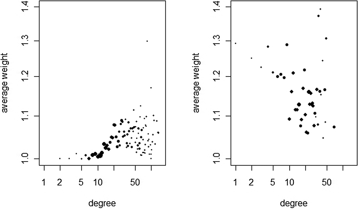
Correlation of degree and average weight for the director (left side) and board network (right side).

The tuning parameter $α$ for the weighted centrality measures depends on the importance of tie strength for the focal phenomena. In particular, betweenness centrality is associated with control, influence, power (Brass, 1984; Hochberg, Ljungqvist, & Lu, 2007; Krackhardt, 1990), and knowledge transfer (Gilsing, Nooteboom, Vanhaverbeke, Duysters, & van den Oord, 2008; Raz & Gloor, 2007), based on control of information flows. The relevance of weak or strong ties depends on the search for or transfer of knowledge, as well as knowledge characteristics (Granovetter, 1973; Hansen, 1999). Weak ties thus provide access to codified knowledge, and an $α$ less than 1 is suitable, whereas strong ties are better suited for the transfer of tacit knowledge, and an $α$ greater than 1 would be a better choice. The comparison of centrality measures for various values of $α$ can help identify actors whose centrality changes with greater tie strength.

Figure 5 shows the correlation of betweenness centrality with weighted betweenness centrality for three different values of the tuning parameter α, as well as the correlation of the weighted measure for α = .5 and 1, normalized by the nonweighted betweenness centrality for the director network. The weighted betweenness centralities for tuning parameters of .5 and 1 correlate positively with the betweenness centrality (correlation coefficients of .97 and .91, respectively), whereas for α = .5 and 1, the correlation is much smaller. In particular, directors with betweenness centrality values between 100 and 100,000 exhibit much lower values for the weighted betweenness centrality. Similarly, Opsahl and Panzarasa (2009) find in the EIES data set of social network researchers that unweighted and weighted measures correlate highly, but a few actors exhibit huge changes across the two measures. Closeness centrality (not shown) reveals similar outcomes for board networks.

Figure 5.

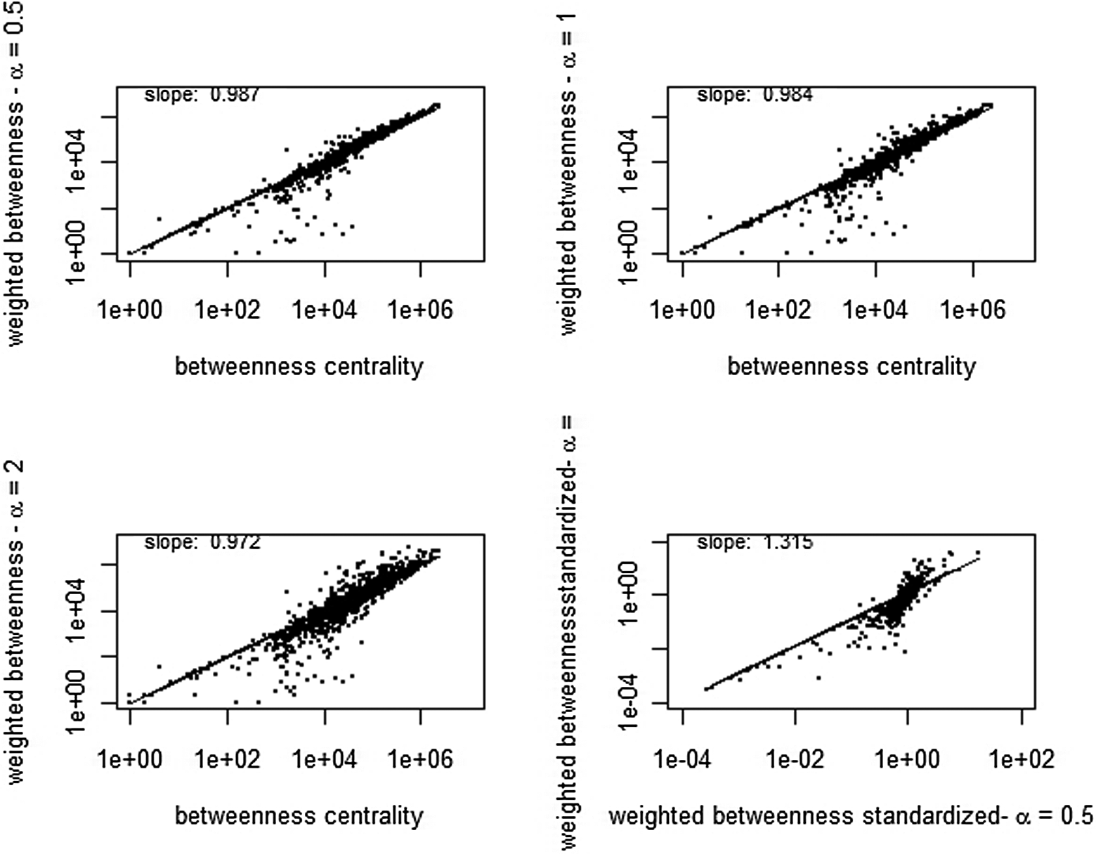
Correlation of betweenness centrality and weighted betweenness centrality for the director network for α = .5, 1, and 2 and the correlation for weighted betweenness for α = .5 and 2.

To illustrate the differences between the unipartite and bipartite clustering coefficient and the impacts of weighting, in Figure 6 we depict their correlation (the tie weights are co-occurrence weights). Although correlated, the bipartite clustering coefficient is generally smaller and spreads over a larger range as the unipartite coefficient increases. The difference is particularly pronounced for a unipartite value of 1, where the bipartite coefficient ranges from .18 to .96.

Figure 6.

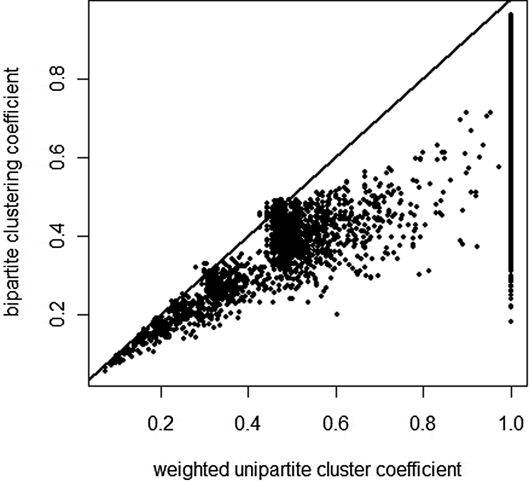
Correlation between weighted unipartite clustering and bipartite clustering coefficients.

For both unipartite and bipartite networks, the unit of analysis could be the node, the dyad, or the whole network. Thus far, we have illustrated node-specific characteristics that can be used as variables in regression analyses. To assess network properties, either the network itself or distributions of node characteristics may be compared against random networks. We therefore compare the distribution of clustering coefficient with random networks, as well as the small-world property and nestedness of the board network.

Table 3 shows the empirical clustering coefficient, the theoretical value in a unipartite network, the NSW coefficient with Newman et al.’s (2001) correction, the resulting small-world coefficient for the simple unipartite network analysis, and the NSW correction of the small-world coefficient. The empirical clustering coefficient for the director network is close to 1 (.90 and .93), reflecting cliques created by the projection. This rather large value sits in stark contrast with the very small theoretical value for unipartite networks, for which we assume independent tie formation. The NSW approach closely reproduces the clustering coefficient of the empirical network. The naive small network analysis would result in a small-world coefficient much larger than 1, suggesting that the Indian board network is a small world. Yet the NSW analysis results in a small-world coefficient close to (and even smaller than) 1, suggesting that this network is not actually a small world and rather that the extensive clustering is a result of the projection of the bipartite network. Similar results arise for the board projection. These results also hold for the full network as well as the giant component. This analysis suggests that the Indian board network is not a small world, in line with findings for other board networks (Conyon & Muldoon, 2006), but it is based on the degree distribution of directors and boards and thus uses the FRFC random network as benchmark. The FRFC suffers from rather large Type II errors, so this conservative test may lead to a failure to reject a false null hypothesis.

Table 3.

Small-World Characteristics for Full Network (full) and Giant Component (gc).

	Empirical clustering coefficient	Theoretical clustering coefficient	NSW clustering coefficient	Small-world coefficient	NSW small-world coefficient
Directors (full)	0.93	3.18E-04	0.57	3,298.62	0.91
Directors (gc)	0.9	5.89E-04	0.49	1,472.43	0.79
Boards (full)	0.45	2.20E-04	0.36	252.37	0.78
Boards (gc)	0.44	2.73E-04	0.28	184.25	0.82

Demonstrating the nestedness of the board network is less suitable because the concept of nestedness is based on generalists and specialists, with many and few nodes, and thus a large variation in degree. As we show in Table 3, most directors serve on only one board. A more promising network appears in the affiliation of firms with specific industries and business groups. We therefore construct a business group–industry network, in which firms associated with a certain business group or industry are linked by a tie. Groups with only firms associated with one industry are not considered. The resulting bipartite network contains 171 business groups and 86 industries. The most generalist business group, with the largest degree, features commercial enterprises of the government, involved in 23 industries, followed by the Tata group, with 18 industries.

In Table 4 we compare the nestedness of the business group–industry network with those of four null models: an FD model with the same density, an FR model that maintains the degree distribution for rows (business groups), an FC model that retains the degree distribution for columns (industries), and the PRC model based on the combined row and column probabilities. Although the nestedness of the empirical network is rather low (7.44), it is significantly larger (p < .001) than those of the FD (4.07), FR (3.74), and PRC (5.76) null models. The rather small value indicates that the nestedness of the system is not very pronounced. Furthermore, the nestedness of the null model that preserves the degree distribution for the columns (i.e., industries) shows a significantly higher nestedness than the empirical network, indicating the importance of the choice of null models.

Table 4.

Nestedness of Business Group–Industry Network in Comparison With Four Random Networks.

Empirical network	Model R00	Model R0	Model C0	Model PRC
7.44	4.07***	3.74***	8.25***	5.76***

Note: PRC = probability row and column.

***p < .001.

Discussion

Summary

We present several recent advances in network analysis that come from outside management literature, with the help of a two-by-two matrix that defines whether the analyzed network is the projected unipartite or original bipartite and whether the analysis pertains to the node level or the network level. We have illustrated several similarities and differences in the applicability of different approaches, using both a simple illustration and a real-world illustration with Indian board networks. Depending on their research question and theoretical objectives, researchers should determine the appropriate methodology accordingly.

Projections of bipartite networks onto unipartite networks should follow two steps to achieve a refined analysis. First, a suitable mechanism is needed to assign weights to the ties in the projection. Second, scholars need to use methods for weighted unipartite networks, such as weighted centrality measures and weighted clustering coefficients, to differentiate network mechanisms on the basis of their weak versus strong ties. A clustering coefficient based on the degree distribution of actor/event nodes can account for natural clustering, as well as the small-world property of projected unipartite networks.

Although weighted unipartite network analysis retains some information, we would still lose information about actors’ connections. To avoid this issue, analyses of an original bipartite network should use bipartite clustering coefficient and nestedness. The bipartite clustering coefficient extends the unipartite concept (based on neighborhoods) and provides a measure of embeddedness in the bipartite network. Nestedness is a bipartite network property that does not have a direct counterpart in the unipartite network analysis. Because nestedness is a unique property of mutualistic networks in ecology, it might serve as a good indicator of the mutual benefits that social networks provide to both types of nodes. Nestedness also may be useful in vertical market relationships, such as in the analysis of the New York garment industry (Saavedra, Reed-Tsochas, & Uzzi, 2009; Saavedra, Stouffer, Uzzi, & Bascompte, 2011). It can be used in situations in which actors are embedded in their environments, such as global trade networks, in which countries exhibit nested structures in product categories (Bustos, Gomez, Hausmann, & Hidalgo, 2012). To advance understanding of nestedness in social systems, further research in collaborative and mutualistic contexts (e.g., coauthorship) would be meaningful.

The measures for weighted networks and the bipartite clustering coefficient can be applied as refined measures of independent variables in regressions, if the unit of analysis is a node. If the unit of analysis is the network, the distribution or aggregation (to the network level) of these measures can be compared against those of appropriate random networks. In bipartite networks, different random networks can serve as null models with various levels of constraints, the choice of which depends on the trade-off between Type I and Type II errors (Gotelli & Entsminger, 2001; Gotelli & Ulrich, 2012). Our illustrations suggest that advanced analytic methods corresponding to different quadrants of the decision matrix (Figure 2) can complement and inform one another, as well as existing measures in unipartite and bipartite network analyses.

We have demonstrated the application of these advanced analytic approaches with two examples: a simple illustration of a bipartite network and a real-life example of the Indian board network in 2009. Our analyses demonstrate that the weighted unipartite network and its centrality measures and clustering carry additional information, making them distinct from the simple analysis of the projected network. Furthermore, the bipartite clustering coefficient differs from its unipartite counterpart and varies widely for given unipartite values, demonstrating the distinction between unipartite and bipartite embeddedness in the network. Our analyses also show that the choice of a random bipartite network is not trivial. The conclusion that the Indian board network is a small world and is nested in its industry structure depends fully on the choice of the random network. The correction of the NSW algorithm suggests that the Indian board network is not a small network, echoing findings by Newman et al. (2001) and Conyon and Muldoon (2006) for board networks of other countries. However, the bipartite degree distribution feeding into the algorithm may be too strong a constraint, leading to acceptance of a false null hypothesis of not being a small world. Researchers must remain aware of these intricacies in their study designs and make informed choices.

Recommendations

How can management scholars make the best use of these new methods? First, in most cases, we are interested in either the antecedents or the consequences of the network structure, but understanding the network topology provides important insights into the object of the investigation. A structural analysis of both types of the nodes also reveals key properties of the network and accounts for interdependence in the two types of nodes. Second, a comparison with random networks supports a determination of whether a network property provides information about the network or is a mere reflection of its basic parameters. In a bipartite network, the proper choice of the random network is crucial; a less constrained random network requires theoretical justification. Third, we focused here on the structural analysis, but the new measures can serve as explanatory variables too. Further research should test how they influence network consequences. Fourth, the enhanced bipartite measures provide additional means for a bipartite network analysis.

Comparability across studies would make it easier to transfer knowledge across fields and disciplines. For example, the unipartite clustering coefficient appears in innovation network studies as the local density of the focal node (Obstfeld, 2005). Understanding the equivalence of clustering coefficients and density measures suggests several new avenues for network research. For example, it would be worthwhile to note similarities in analyses of bipartite networks with research on population ecology. Population ecologies entail bipartite networks with organizations and niches; other concepts, such as niche width and generalist or specialist, might be expressed as notions of these bipartite networks. This conceptualization suggests new avenues for analysis (e.g., nestedness), as well as cross-disciplinary knowledge accumulation.

Researchers can use the analytic tools available for different quadrants in Figure 2 to compare networks across different disciplines. Measures of overlap, such as niche or technological overlap, represent different types of bipartite clustering coefficients. This insight may facilitate the conceptualization and analysis of populations as bipartite networks. Finally, a greater focus on the properties of bipartite networks would improve our understanding of the network itself, as well as inform node- and dyad-level analyses and perhaps spur more research on bipartite measures and random networks.

In summary, a proper understanding of unipartite and bipartite networks can help scholars analyze networks at different levels. In many cases, the bipartite structure stretches across two levels, such as individuals and groups or directors and boards, and thus can be used to derive multilevel measures at the individual (actor) or group (event) level. Conducting an analysis at the node and network levels enables scholars to examine local and global phenomena simultaneously. Acknowledging the bipartite nature of networks and the application of the advanced measures also might accelerate the accumulation of knowledge for management field.

Footnotes

Appendix A

The generating function for the degree distribution is 10

G_{0} (x) = \sum_{k = 0}^{\infty} p_{k} x^{k} w i t h G_{0} (1) = 1 a n d ⟨ k ⟩ = \sum_{k}^{\infty} k p_{k} = G_{0}^{^{'}} (1),

where

G_{0} (1) = 1

ensures that all the probabilities

p_{k}

add to 1 and the average degree is expressed in terms of the first derivative of the generating function. For an observed network, the probabilities

p_{k}

can be directly measured by the degree distribution of the network

n_{k}

, where

n_{k}

is the number of nodes with degree k. In this case, the generating function is obtained by 11

G_{0} (x) = \frac{\sum_{k} n_{k} x^{k}}{\sum_{k} n_{k}} .

In a bipartite network, there are two generating functions $f_{0}$ and $g_{0}$ , such that $f_{0}$ generates the Type 1 network (e.g., directors) and $g_{0}$ produces the Type 2 network (e.g., boards). Thus, 12

f_{0} (x) = \sum_{j} p_{j} x^{j}, g_{0} (x) = \sum_{k} q_{k} x^{k},

and as in the case of the unipartite case, the following relations hold 13

f_{0} (1) = g_{0} (1) = 1, f {^{'}}_{0 (1)} = μ, g {^{'}}_{0 (1)} = ν .

Here, µ and ν are the average number of node types in the network. Newman, Strogatz, and Watts (2001) derived formulas for the average path length L and the clustering coefficient $C_{G}$ from the two generating functions: 14

L = \frac{l n (\frac{N}{z_{1}})}{l n (\frac{z_{2}}{z_{1}})} + 1

with 15

z_{1} = G_{0}^{'} (1) = f_{0}^{'} g_{0}^{'} (1), z_{z} = G_{0}^{'} (1) G_{1}^{'} (1) = f_{0}^{'} (1) f_{1}^{'} (1) {[g_{1} (1)]}^{2}

C_{G} = \frac{M}{N} \frac{g_{0}^{^{'''}} (1)}{G_{0}^{^{''}} (1)},

where N is the number of Type 1 nodes and M is the number of Type 2 nodes.

Our goal is not to provide the detailed derivation of Equations 14 through 16 but rather to describe their applications to bipartite networks. We therefore provide explicit formulas for the derivatives in Equations 14 through 16 by applying the chain rule to calculate the derivatives and substitute x = 1, as follows:

f_{0}^{'} = \sum_{j} j p_{j} x^{j - 1} f_{0}^{'} (1) = μ

f_{0}^{''} (x) = \sum_{j} j (j - 1) p_{j} x^{j - 2} f_{0}^{''} (1) = \sum_{j} j (j - 1) p_{j}

f_{1}^{'} (x) = \frac{1}{μ} \sum_{j} j (j - 1) p_{j} x^{j - 2} f_{1}^{'} (1) = \frac{1}{μ} \sum_{j} j (j - 1) p_{j}

g_{0}^{'''} (x) = \sum_{k} k (k - 1) (k - 2) q_{k} x^{k - 3} g_{0}^{'''} (1) = \sum_{k} k (k - 1) (k - 2) q_{k}

g_{1}^{'} (x) = \frac{1}{v} \sum_{k} k (k - 1) q_{k} x^{k - 2} g_{1}^{'} (1) = \frac{1}{v} \sum_{k} k (k - 1) q_{k}

G_{1}^{'} (x) = f_{1}^{'} (g_{1} (x)) g_{1}^{'} (x) G_{1}^{'} (1) = f_{1}^{'} (1) g_{1}^{'} (1)

G_{0}^{''} (x) = {f_{0}}^{''} (g_{1} (x)) [g_{1}^{'} (x)]^{2} + f_{0}^{'} (g_{1} (x)) g_{1}^{'} (x) G_{0}^{''} (1) = {f_{0}}^{''} (1) (g_{1}^{'} (x))^{2} + μ g_{1}^{''} (1) .

With the derivatives evaluated for x = 1, we can calculate the average path length and the clustering coefficient as a sum of the products of the empirical probabilities $p_{j}$ and $q_{k}$ with the degree distribution.

We provide an explicit example of the calculation of the clustering coefficient as defined by Newman et al. (2001) for the giant component of the Indian board network in Table A1. The values of the line with the column sums can be plugged into Equation 23, which yields $G_{0}^{''} = 83.55 \cdot {1.08}^{2} + 9.1 \cdot 4.08 = 134.6.$ Thus, we obtain a clustering coefficient from Equation 16, with $C_{G} = \frac{10223}{1528} \frac{5.55}{134.6} = 0.276$ .

Appendix B

Acknowledgments

The authors thank Chuck Pierce, Vikas Kumar, Debmalya Mukherjee, and participants at the 2012 Academy of Management Conference for comments on previous versions. This article benefited greatly from comments and advice provided by Associate Editor Adam Meade and three anonymous reviewers.

Declaration of Conflicting Interests

The author(s) declared no potential conflicts of interest with respect to the research, authorship, and/or publication of this article.

Funding

The author(s) disclosed receipt of the following financial support for the research, authorship, and/or publication of this article: This research was supported by grants from Rutgers University Research Council and the Technology Management Research Center of Rutgers Business School.

References

Almeida-Neto

Guimãres

P. R.

Jr Loyola

R. D.

Ulrich

(2008). A consistent metric for nestedness analysis in ecological systems: Reconciling concept and measurement. Oikos, 117(8), 1227–1239.

Atmar

Patterson

B. D.

(1993). The measure of order and disorder in the distribution of species in fragmented habitat. Oecologia, 96, 373–382.

Barrat

Barthélemy

Pastor-Satorras

Vespignani

(2004). The architecture of complex weighted networks. Proceedings of the National Academy of Sciences of the United States of America, 101(11), 3747–3752.

Bascompte

Jordano

(2007). Plant-animal mutualistic networks: The architecture of biodiversity. Annual Review of Ecology, Evolution & Systematics, 38(1), 567–593.

Bascompte

Jordano

Melin

C. J.

Olesen

J. M.

(2003). The nested assembly of plant-animal mutualistic networks. Proceedings of the National Academy of Sciences of the United States of America, 100(16), 9383–9387.

Battiston

Catanzaro

(2004). Statistical properties of corporate board and director networks. European Physical Journal B–Condensed Matter, 38(2), 345–352.

Baum

J. A. C.

Shipilov

A. V.

Rowley

T. J.

(2003). Where do small worlds come from? Industrial & Corporate Change, 12(4), 697–725.

Borgatti

S. P.

Everett

M. G.

(1997). Network analysis of 2-mode data. Social Networks, 19(3), 243–269.

Borgatti

S. P.

Halgin

D. S.

(2011). On network theory. Organization Science, 22(5), 1168–1181.

10.

Brandes

(2001). A faster algorithm for betweenness centrality. Journal of Mathematical Sociology, 25(2), 163–177.

11.

Brass

D. J.

(1984). Being in the right place: A structural analysis of individual influence in an organization. Administrative Science Quarterly, 29(4), 518–539.

12.

Breiger

R. L.

(1974). The duality of persons and groups. Social Forces, 53(2), 181–190.

13.

Breiger

R. L.

Mohr

J. W.

(2004). Institutional logics from the aggregation of organizational networks: Operational procedures for the analysis of counted data. Computational and Mathematical Organization Theory, 10(1), 17–43.

14.

Bustos

Gomez

Hausmann

Hidalgo

C. A.

(2012). The dynamics of nestedness predicts the evolution of industrial ecosystems (CID Working paper No. 236). Cambridge, MA: Harvard University.

15.

Carroll

G. R.

(1985). Concentration and specialization: Dynamics of niche width in populations of organizations. American Journal of Sociology, 90(6), 1262–1283.

16.

Chung

Singh

Lee

(2000). Complementarity, status similarity and social capital as drivers of alliance formation. Strategic Management Journal, 21(1), 1–22.

17.

Conaldi

Lomi

Tonellato

(2012). Dynamic models of affiliation and the network structure of problem solving in an open source software project. Organizational Research Methods, 15(3), 385–412.

18.

Conyon

M. J.

Muldoon

M. R.

(2006). The small world of corporate boards. Journal of Business Finance & Accounting, 33(9), 1321–1343.

19.

Csardi

Nepusz

(2006). The igraph software package for complex network research. InterJournal, Complex Systems, 1695–1704.

20.

Davis

G. F.

Yoo

Baker

W. E.

(2003). The small world of the American corporate elite, 1982-2001. Strategic Organization, 1(3), 301–326.

21.

Dionne

S. D.

Akaishi

Chen

Gupta

Sayama

Yammarino

F. J.,

… Bush

B. J.

(2012). Retrospective relatedness reconstruction: Applications to adaptive social networks and social commitment. Organizational Research Methods, 15(4(, 663–692.

22.

Dormann

C. F.

Gruber

Fründ

(2008). Introducing the bipartite package: Analysing ecological networks. R News, 8(2), 8–11.

23.

Erdös

Rényi

(1959). On random graphs. Publicationes Mathematicae, 6, 290–297.

24.

Faust

(1997). Centrality in affiliation networks. Social Networks, 19(2), 157–191.

25.

Fleming

Mingo

Chen

(2007). Collaborative brokerage, generative creativity, and creative success. Administrative Science Quarterly, 52(3), 443–475.

26.

Freeman

Carroll

G. R.

Hannan

M. T.

(1983). Age dependence in organizational death rates. American Sociological Review, 48(2), 692–710.

27.

Gilsing

Nooteboom

Vanhaverbeke

Duysters

van den Oord

(2008). Network embeddedness and the exploration of novel technologies: Technological distance, betweenness centrality and density. Research Policy, 37(10), 1717–1731.

28.

Gotelli

Entsminger

(2001). Swap and fill algorithms in null model analysis: Rethinking the knight’s tour. Oecologia, 129(2), 281–291.

29.

Gotelli

N. J.

Ulrich

(2012). Statistical challenges in null model analysis. Oikos, 121(2), 171–180.

30.

Granovetter

(1973). The strength of weak ties. American Journal of Sociology, 78(6), 1360–1380.

31.

Greve

H. R.

Baum

J. A. C.

Mitsuhashi

Rowley

T. J.

(2010). Built to last but falling apart: Cohesion, friction, and withdrawal from interfirm alliances. Academy of Management Journal, 53(2), 302–322.

32.

Hansen

M. T.

(1999). The search-transfer problem: The role of weak ties in sharing knowledge across organization subunits. Administrative Science Quarterly, 44(1), 82–111.

33.

Hochberg

Y. V.

Ljungqvist

(2007). Whom you know matters: Venture capital networks and investment performance. Journal of Finance, 62(1), 251–301.

34.

Kogut

Belinky

(2008). Comparing small world statistics over time and across countries: An introduction to the special issue comparative and transnational corporate networks. European Management Review, 5(1), 1–10.

35.

Kogut

Urso

Walker

(2007). Emergent properties of a new financial market: American venture capital syndication, 1960-2005. Management Science, 53(7), 1181–1998.

36.

Krackhardt

(1990). Assessing the political landscape: Structure, cognition, and power in organizations. Administrative Science Quarterly, 35(2), 342–369.

37.

Latapy

Magnien

Vecchio

N. D.

(2008). Basic notions for the analysis of large bipartite networks. Social Networks, 30(1), 31–48.

38.

Lin

Yang

Irem

(2007). The performance consequences of ambidexterity in strategic alliance formations: Empirical investigation and computational theorizing. Management Science, 53(10), 1645–1658.

39.

Lomi

Pallotti

(2012). Relational collaboration among special multipoint competitors. Social Networks, 34, 101–111.

40.

Moody

White

D. R.

(2003). Structural cohesion and embeddedness: A hierarchical concept of social groups. American Sociological Review, 68(1), 103–127.

41.

Newman

M. E. J.

(2001). The structure of scientific collaboration networks. Proceedings of the National Academy of Science, 98, 404–409.

42.

Newman

M. E. J.

Strogatz

S. H.

Watts

D. J.

(2001). Random graphs with arbitrary degree distributions and their applications. Physical Review E, 64(2), 026118.

43.

Obstfeld

(2005). Social networks, the tertius iungens orientation, and involvement in innovation. Administrative Science Quarterly, 50(1), 100–130.

44.

Oksanen

Blanchet

F. G.

Kindt

Legendre

Minchin

P. R.

O’Hara

R. B.,

… Wagner,

(2011). Vegan: Community ecology package. R package version 1.8-3 [Computer software]. Retrieved from http://CRAN.R-project.org/.

45.

Opsahl

(2009). Structure and evolution of weighted networks. Retrieved from http://toreopsahl.com/publications/thesis

46.

Opsahl

Agneessens

Skvoretz

(2010). Node centrality in weighted networks: Generalizing degree and shortest paths. Social Networks, 32(3), 245–251.

47.

Opsahl

Panzarasa

(2009). Clustering in weighted networks. Social Networks, 31(2), 155–163.

48.

Podolny

J. M.

Baron

J. N.

(1997). Resources and relationships: Social networks and mobility in the workplace. American Sociological Review, 62(5), 673–693.

49.

Podolny

J. M.

Stuart

T. E.

Hannan

M. T.

(1996). Networks, knowledge, and niches: Competition in the worldwide semiconductor industry, 1984-1991. American Journal of Sociology, 102(3), 659–689.

50.

R Core Development Team. (2011). R: A language and environment for statistical computing [Computer software]. Vienna, Austria: R Foundation for Statistical Computing.

51.

Raz

Gloor

P. A.

(2007). Size really matters—new insights for start-ups’ survival. Management Science, 53(2), 169–177.

52.

Robins

Alexander

(2004). Small worlds among interlocking directors: Network structure and distance in bipartite graphs. Computational and Mathematical Organization Theory, 10(1), 69–94.

53.

Saavedra

Reed-Tsochas

Uzzi

(2009). A simple model of bipartite cooperation for ecological and organizational networks. Nature, 457(7228), 463–466.

54.

Saavedra

Stouffer

D. B.

Uzzi

Bascompte

(2011). Strong contributors to network persistence are the most vulnerable to extinction. Nature, 478(7368), 233–235.

55.

Schweitzer

Fagiolo

Sornette

Vega-Redondo

Vespignani

White

D. R.

(2009). Economic networks: The new challenges. Science, 325(5939), 422–425.

56.

Ulrich

Almeida-Neto

Gotelli

N. J.

(2009). A consumer’s guide to nestedness analysis. Oikos, 118, 3–17.

57.

Wang

Sharpe

Robins

G. L.

Pattison

P. E.

(2009). Exponential random graph (p*) models for affiliation networks. Social Networks, 31(1), 12–25.

58.

Wasserman

Faust

(1994). Social network analysis. Cambridge, England: Cambridge University Press.

59.

Watts

D. J.

Strogatz

S. H.

(1998). Collective dynamics of “small-world” networks. Nature, 393(6684), 440–442.

60.

White

D. R.

Harary

(2001). The cohesiveness of blocks in social networks: Node connectivity and conditional density. Sociological Methodology, 31, 305–359.

61.

Zaheer

Soda

(2009). Network evolution: The origins of structural holes. Administrative Science Quarterly, 54, 1–31.