Residualized Relative Importance Analysis

Abstract

The current article notes that the standard application of relative importance analyses is not appropriate when examining the relative importance of interactive or other higher order effects (e.g., quadratic, cubic). Although there is a growing demand for strategies that could be used to decompose the predicted variance in regression models containing such effects, there has been no formal, systematic discussion of whether it is appropriate to use relative importance statistics in such decompositions, and if it is appropriate, how to go about doing so. The purpose of this article is to address this gap in the literature by describing three different yet related strategies for decomposing variance in higher-order multiple regression models—hierarchical F tests (a between-sets test), constrained relative importance analysis (a within-sets test), and residualized relative importance analysis (a between- and within-sets test). Using a previously published data set, we illustrate the different types of inferences these three strategies permit researchers to draw. We conclude with recommendations for researchers seeking to decompose the predicted variance in regression models testing higher order effects.

Keywords

multiple regression quantitative research interactions measurement models relative weight analysis dominance analysis

Within the organizational sciences, multiple regression continues to be one of the most popular data analytic techniques. For example, Podsakoff and Dalton (1987) found that regression was used in 14.24% of the empirical articles published in the top-tier Industrial-Organizational Psychology/Organizational Behavior journals in 1985. Stone-Romero, Weaver, and Glenar (1995) reviewed articles published in the Journal of Applied Psychology from 1975 to 1993 and found that the frequency of using regression increased over that period. Similarly, Scandura and Williams (2000) reported that the number of empirical studies in which regression was used significantly increased from 30.70% in 1985-1987 to 42.40% in 1995-1997. More recently, a review of the work–family literature found that roughly 53% of studies relied on some form of regression analysis (Casper, Eby, Bordeaux, Lockwood, & Lambert, 2007). This finding is consistent with a more general review of articles published in the Journal of Applied Psychology, which found that 46% of the articles published in 2000 relied on some form of regression analysis (Austin, Scherbaum, & Mahlman, 2002). Finally, Aguinis, Pierce, Bosco, and Muslin (2008) found that regression remained the most popular topical area in methodological articles (17.03% of 193 articles) published in Organizational Research Methods from 1998 to 2007. Collectively, these reviews indicate that multiple regression has been, and continues to be, one of the most important data analytic frameworks in the organizational sciences.

The popularity of multiple regression is likely, at least in part, a result of the flexibility of this analytic framework for testing a variety of statistical models. Researchers have used multiple regression to test models containing simple additive effects, as well as models containing interactive and higher order polynomial effects (cf. Aiken & West, 1991; Bing, LeBreton, Davison, Migetz, & James, 2007; Cortina, 1993; Edwards, 1994, 2002; Edwards & Parry, 1993; Ployhart & Hakel, 1998; Podsakoff & Dalton, 1987). In addition, multiple regression is popular because it may be used for the dual purposes of prediction (e.g., developing and testing models having nontrivial R² values) and explanation (e.g., trying to understand which predictors are driving that nontrivial R²; Pedhazur, 1997).

Researchers pursuing these two goals have historically focused on two key aspects of multiple regression: (a) estimating the overall model R² and (b) determining the statistical significance of individual regression coefficients. The overall R² informs us as to the proportion of variance explained in our dependent variable or criterion. The estimate of R² can be tested for statistical significance and interpreted as a general measure of effect size (Cohen, Cohen, West, & Aiken, 2003; Pedhazur, 1997). The statistical significance of individual regression coefficients informs us as to the incremental predictive validity of the predictor variables. This is useful because it lets a researcher understand the unique contribution a variable makes to that R². However, it is not uncommon that a variable demonstrates a highly significant bivariate relationship with the criterion, whereas this variable’s regression coefficient suggests a small or nonsignificant increment in variance explained. Thus, a small or even nonsignificant incremental effect size does not necessarily imply that the predictor is unimportant or irrelevant to one’s theory or model (Cortina & Landis, 2009; LeBreton, Hargis, Griepentrog, Oswald, & Ployhart, 2007).

One way to ascertain the importance or contribution of predictor variables is through a third aspect of multiple regression that Darlington (1968) highlighted in his seminal article on regression—determining the relative importance of predictors. Relative importance is defined as the contribution each individual variable makes to the R² when that variable is considered by itself (i.e., independent effect) and in combination with other variables (i.e., conditional effect; J. W. Johnson & LeBreton, 2004). Darlington noted that when one has orthogonal predictors, ascertaining the relative importance of these predictors is straightforward and unambiguous. One could use squared correlation coefficients (r²), squared standardized regression coefficients (β²), the products of the correlation and standardized regression coefficients (rβ), or the “usefulness” of the variable, which is defined as the change in variance explained as a variable is added or removed from the regression (ΔR²). However, he also noted that when predictors were correlated, none of the extant statistics provided an acceptable decomposition of the total predicted variance (R²). Thus, determining the relative importance of correlated predictors was not possible. This problem would continue to plague applied psychology for the next 25 years. During this time, psychologists continued to rely on the less-than-optimal estimates of incremental validity or standardized regression weights.

It was not until the introduction of dominance analysis (DA; Budescu, 1993) and relative weight analysis (RWA; J. W. Johnson, 2000) that substantial progress was made toward understanding the relative contribution that correlated predictors make to the overall predictive power of a regression model. Although based on very different statistical rationale, these two procedures were both designed to provide meaningful estimates of relative importance in the presence of correlated predictors. To date, the accumulated evidence supports the conclusion that these procedures do in fact provide such estimates, even with correlated predictor variables (cf. Azen & Budescu, 2003; Budescu, 1993; Budescu & Azen, 2004; J. W. Johnson, 2000, 2001; J. W. Johnson & LeBreton, 2004; Krasikova, LeBreton, & Tonidandel, 2011; LeBreton, Binning, Adorno, & Melcher, 2004; LeBreton et al., 2007; LeBreton, Ployhart, & Ladd, 2004; LeBreton & Tonidandel, 2008; Tonidandel & LeBreton, 2010, 2011; Van Iddekinge & Ployhart, 2008).

Failure to consider these newer indices of relative importance can lead researchers to misconstrue the true contribution of variables in their regression models, which can slow the progress of empirical research and hinder theory development. For example, Courville and Thompson (2001) reviewed articles in the Journal of Applied Psychology over an 11-year span and identified frequent errors made by authors who used regression weights to determine the relative importance of correlated predictors. Fortunately, there is growing consensus that the information provided by relative importance analyses is instrumental to having a comprehensive understanding of which variables are contributing to (i.e., driving) the explanatory power of a regression model (cf. Azen & Budescu, 2003; J. W. Johnson & LeBreton, 2004; Krasikova et al., 2011; Tonidandel & LeBreton, 2011; Van Iddekinge & Ployhart, 2008). As a consequence, DA and RWA are now regularly used to supplement the information obtained from a traditional regression analysis and are seeing increased use in the organizational sciences (cf. Colquitt, LePine, Piccolo, Zapata, & Rich, 2012; Eby, Butts, & Lockwood, 2003; Glomb, Kammeyer-Mueller, & Rotundo, 2004; Jackson, Colquitt, Wesson, & Zapata-Phelan, 2006; James, 1998; J. W. Johnson, 2001; R. E. Johnson, Tolentino, Rodopman, & Cho, 2010; LeBreton et al., 2004; Lievens, Conway, & De Corte, 2008; Lievens, Highhouse, & De Corte, 2005; Luo, 2005; McAllister, Kamdar, Morrison, & Turban, 2007; Morgeson & Nahrgang, 2008; Nickerson, Schwarz, Diener, & Kahneman, 2003; Schleicher, Venkataramani, Morgeson, & Campion, 2006; Tonidandel & LeBreton, 2011; Van Iddekinge & Ployhart, 2008).

Since relative importance analysis can play an instrumental role in guiding our interpretation of the impact of predictors, it becomes necessary to provide researchers with the tools that will allow performing relative importance analysis across the wide variety of situations they are likely to encounter. The world of psychology is not always a simple, main-effects world. As organizational researchers continue to use more sophisticated regression models attempting to test the complexities of the real world, they often must examine interactive and higher order polynomial effects (Aguinis, 2004; Aguinis, Beaty, Boik, & Pierce, 2005; Aiken & West, 1991; Edwards, 2002; Edwards & Parry, 1993; MacCallum & Mar, 1995).

For example, Glomb et al. (2004) used multiple regression analysis to test the relationship between emotional labor and various job demands in the prediction of job compensation. Specifically, the authors examined main effects, quadratic effects, and interaction effects, linking emotional labor, physical job demands, and cognitive job demands in the prediction of hourly wages. Although they were able to examine the relative importance of the main effects, they were unable to examine the relative importance of the quadratic or interaction effects. This is not meant as a criticism of their work. On the contrary, they were using the most cutting-edge statistical tools available at that time. Unfortunately, those tools were limited in the types of inferences that could be drawn.

Specifically, no statistical tools exist that permit researchers to simultaneously partition the predicted variance in the criterion among both lower-order and higher order effects. Lacking such tools, researchers are not able to appreciate the relative contribution that various effects make to their understanding of organizational phenomena. As we illustrate later in our article, reliance on statistical significance tests of individual regression terms can be misleading. However, coupling significance testing with relative importance analyses can provide for a more enlightened evaluation of the variables used to test our theories.

The purpose of this article is to address these gaps in the literature. In the following sections we (a) overview the use of relative importance statistics to decompose the variance in traditional additive regression models (i.e., models containing only main effects), (b) briefly discuss how multiple regression may be used to test for interactive, quadratic, and other higher order effects, and (c) discuss three different yet related strategies for decomposing variance in higher order multiple regression models. Throughout this discussion, we rely on the results from actual data to highlight types of inferences researchers may draw when using each of these three strategies. However, before continuing, it is important to delimit what we mean by the term importance and how our use is related to other uses of this term in the statistical literature.

Importance connotes different meanings, depending on the situation. Sometimes importance refers to whether concomitant variation between two variables exceeds what would be expected based on chance. Here, variable importance is equated with statistical significance. Another commonly used definition of importance equates a variable’s importance to the practical impact a variable has on the criterion. Variable importance, when used in this way, considers both the effect size associated with a particular variable along with the specifics of the situation surrounding the use of that variable. Cortina and Landis (2009) and others (e.g., LeBreton et al., 2007; Martell, Lane, & Emrich, 1996) have appropriately recognized that, in particular situations, large effects may have little practical utility, whereas in other situations, relatively small effects can be quite meaningful. In contrast to these two prior definitions, our use of the term importance coincides with the historical statistical usage of this term, which equates importance to the amount of variance each individual variable contributes to R² (Darlington, 1968) when a variable is considered by itself and with the other variables. Because our definition of relative importance considers only the statistical contribution of each variable to total predictable variance irrespective of context, practical utility of a variable is not addressed by relative importance analysis.

These three definitions of importance should not be viewed as mutually exclusive. Instead, as we show later, they assess different aspects of importance, each of which we believe should be considered when researchers test their theories. With that caveat in place, we now proceed with a discussion of variance decomposition (i.e., estimating relative importance) within the context of a first-order linear regression model before discussing how such decompositions may be conducted in higher order models.

Decomposing Variance in the First-Order Multiple Linear Regression

With a first-order linear regression model, a relative importance analysis is ideally suited to decompose the predicted variance in the criterion into that attributed to each individual predictor (i.e., main effect). As noted above, relative importance is defined as the contribution each predictor makes to the R² when that predictor is considered by itself (i.e., independent effect) and in combination with other predictors (i.e., conditional effect; J. W. Johnson & LeBreton, 2004).

For years, researchers sought techniques for decomposing the predicted criterion variance and at various times have relied on squared bivariate correlations, squared standardized regression coefficients, and the products of the correlation and the standardized regression coefficients (see J. W. Johnson & LeBreton, 2004, for a detailed review). When the predictors are orthogonal, virtually all techniques yield identical estimates of importance; however, when the predictors are correlated, each of the aforementioned approaches to estimating relative importance is limited, and thus, the results may diverge quite dramatically (Budescu, 1993; Darlington, 1968; J. W. Johnson, 2000; LeBreton et al., 2004). In an attempt to overcome the various limitations of these past indices, researchers have developed two statistics designed for use with correlated predictors: general dominance weights and relative weights.

General Dominance Weights

DA addresses the problem of correlated predictors by examining the additional contribution each predictor makes across all subset regressions (Azen & Budescu, 2003; Budescu, 1993). Mathematically, general dominance weights are obtained for each of the J predictors by averaging the ΔR² obtained by adding each predictor variable to all possible subsets of the remaining predictor variables. Specifically, the initial ΔR² of a variable by itself is first examined. Then, the ΔR² (i.e., incremental validity) of the focal variable is examined when that variable is added to a regression equation containing each of the other variables. This process continues by examining ΔR² resulting from adding the focal variable to all combinations of two variables, three variables, and so on, and the results are then averaged. Stated alternatively, general dominance weights are equal to variables’ average squared semipartial correlations across all subset regressions. A separate general dominance weight is computed for each of the J predictor variables and is denoted C_j .

Relative Weights

RWA addresses the problem of correlated predictors using a variable transformation approach (J. W. Johnson, 2000). Specifically, relative weights, denoted ∊_j , are estimated by creating a series of new predictors (Z_k ) that are the maximally related (in a least squares sense) orthogonal counterparts of the original predictors (X_j ). These new orthogonal variables are then used in tandem with the original correlated predictors to estimate relative weights. First, a researcher regresses the criterion (Y) on the new uncorrelated predictor variables (Z_k ) to obtain standardized regression coefficients (β _k ). Next, he or she regresses the original correlated predictors (X_j ) on their orthogonal counterparts (Z_k ) to obtain the standardized regression coefficients (λ _jk ). Finally, β _k s and λ _jk s are squared and combined with one another using the matrix algebra equations presented in J. W. Johnson (2000).

RWA and DA have become the preferred analytic strategies for decomposing the predicted criterion variance in first-order regression models (J. W. Johnson & LeBreton, 2004; Tonidandel & LeBreton, 2011). The importance weights furnished by these analyses are scaled in the metric of relative or conditional effect sizes (LeBreton et al., 2007). In addition, a desirable statistical property of estimates of variable importance is that they should sum to the model R² (Darlington, 1968). Both relative weights and general dominance weights possess this property (Azen & Budescu, 2003; J. W. Johnson & LeBreton, 2004; Krasikova et al., 2011). Consequently, it is possible to calculate rescaled importance weights by dividing the general dominance weights or the relative weights by the model R² and then multiplying these values by 100. The resultant rescaled weights are interpreted as the percentage of predicted criterion variance attributed to each variable. Although general dominance weights and relative weights are predicated on completely different statistical rationales, they have been shown to yield virtually identical results in both simulation studies (e.g., LeBreton et al., 2004) and primary studies (e.g., J. W. Johnson, 2000). It is for all of these reasons that these two approaches have been recommended for decomposing predicted criterion variance when one has correlated predictors (J. W. Johnson & LeBreton, 2004). However, as we explain later in our article, both approaches in their current form are inappropriate for decomposing the predicted variance in models testing interactive and other higher order effects.

Estimating and Testing Interactive and Other Higher Order Effects

Given the flexibility of multiple regression analysis, it is often the preferred framework for testing interaction effects (Aiken & West, 1991) and other higher order polynomial effects (Edwards, 1994, 2002; Edwards & Parry, 1993). For ease of exposition, we assume that (a) we are dealing with continuous variables, (b) all variables have been standardized, and (c) any cross-products (or higher order terms) have been appropriately computed as the cross-product of standardized variables and not the standardization of the raw variable cross-product (Cohen et al., 2003). The extension to categorical variables is straightforward, as we illustrate later in our example. That said, the standard approach to testing for interactions involves estimating a series of hierarchical regression models that are typically described under the umbrella term moderated multiple regression (MMR). We begin with a main effects model where the dependent variable Y is regressed on the predictors carrying the main effects U and V.¹

Y = β_{1} U + β_{2} V + e .

This yields standardized regression coefficients β ₁ and β ₂ and an error term, e, which is typically assumed to be independently and identically distributed with mean zero and constant variance. This model provides a baseline estimate of whether either or both predictor variables exert a main effect on Y and an estimate of the amount of variance in Y explained by the two main effects (Model 1 R²). Next, the cross-product between U and V, denoted UV, is added:

Y = β_{0} + β_{1} U + β_{2} V + β_{3} U V + e .

Equation 2 yields the standardized regression coefficient β ₃, which indexes the extent to which the cross-product term predicts above and beyond the main effects. It is worth mentioning that the mean of the cross-product of standardized variables will rarely be zero, thus the intercept, β ₀, is reintroduced in this equation. Equation 2 also yields a new estimate of variance explained (Model 2 R²), which can be compared to the previous variance explained (i.e., ΔR² = Model 2 R² – Model 1 R²).

Before continuing, it is critical for us to clarify what we mean by regression terms and regression effects. A regression term is a variable (predictor) entered into a regression equation. For example, U represents the linear term, whereas U² represents the quadratic term (i.e., U multiplied by U), and UV represents the cross-product term (i.e., U multiplied by V). In contrast, a regression effect refers to the impact that a regression term exerts on Y, after appropriately controlling for (i.e., residualizing for) other relevant effects. In the first-order linear regression, regression terms are isomorphic with regression effects. However, things change when we move to higher order effects. For example, we use U² _r.U to represent the quadratic effect (i.e., the effect of U² on Y after controlling for the main effect of U) and UV_{r.U, V} to represent the interaction effect (i.e., the impact of UV after controlling for the main effects of U and V).

When testing an interaction effect, we adhere to a strict hierarchy of precedence—main effects (linear terms) are entered prior to testing the cross-product term. Conducting a hierarchical test is necessary because the cross-product term (UV) is a tainted, messy predictor containing information about three different statistical effects: (a) the main effect of U, (b) the main effect of V, and (c) the UV interaction effect (i.e., UV_{r.U, V} ; Aiken & West, 1991). There are two ways to get a “clean” estimate of this interaction effect. The first approach is to rely on the hierarchical analysis described earlier. The second approach, which is mathematically equivalent to the first approach, is to simply calculate the appropriate interaction term by regressing the cross-product on the two predictors and saving the residuals. This latter approach creates an interaction term that is isomorphic with the interaction effect. We revisit this approach later in the article when discussing strategies for estimating the relative importance of interactive and other higher order effects.

This hierarchy of precedence becomes even more complicated if we adopt Cortina’s (1993) recommendation and include an intermediate model containing the quadratic terms U² and V ². His recommendation stems from concern over detecting a spurious interaction effect (UV_{r.U, V} ) that may simply represent one of the quadratic effects (U² _r.U or V ² _r.V ; also see Ganzach, 1998; Lubinski & Humphreys, 1990). Cortina’s (1993) approach is congruent with the work by Lubinski and Humphreys (1990), Shepperd (1991), MacCallum and Mar (1995), and Ganzach (1997, 1998) advocating the inclusion of quadratic terms in regression models with correlated predictors when interaction effects are of interest. If researchers adopt the recommendation that quadratic effects should be included prior to testing interaction effects, they would begin with the model presented in Equation 1 and add the quadratic terms,

Y = β_{0} + β_{1} U + β_{2} V + β_{3} U^{2} + β_{4} V^{2} + e,

where U² and V ² are obtained by multiplying each independent variable by itself. This regression yields an estimate of the variance explained in Y by main effects and quadratic effects (Model 3 R²). This model is also hierarchical in that the linear terms are entered first followed by the quadratic terms because each quadratic term contains information about its corresponding main effect. We continue by adding the cross-product:

Y = β_{0} + β_{1} U + β_{2} V + β_{3} U^{2} + β_{4} V^{2} + β_{5} U V + e .

This final model provides individual parameter estimates for the main, quadratic, and interactive effects, but also an estimate of the variance explained in Y by these effects (Model 4 R² produced by Equation 4), which can be compared to the previous variance explained (Model 3 R² produced by Equation 3). The significance of the ΔR² may be tested using the equations presented in Cohen et al. (2003), and it is statistically equivalent to the test of regression coefficient β ₅ in Equation 4.

To summarize, if a researcher uses a cross-product term to test for an interaction effect, it is first necessary to control for any additional effects carried by that cross-product. By extension, if a researcher wished to test the three-way interaction UVW, it would be necessary to control for the three main effects and the three two-way interactive effects before examining the significance of the three-way interactive effect. And if a researcher uses a higher order polynomial term to test for quadratic, cubic, or quartic effects, it would again be necessary to first control for all lower order effects included in that polynomial term. Thus, if someone wished to test the cubic effect, U³ _{r.U, U} ², he or she would first need to control for the main and quadratic effects.

These conclusions may not seem profound and have been discussed extensively in the literature; however, they have important consequences for how one goes about decomposing the explained variance in a regression model containing higher order effects. Specifically, the two leading approaches for estimating relative importance, DA and RWA, rely on an unrestricted regression model where there is no inherent ordering of the variables (Budescu, 1993; J. W. Johnson, 2000). That is, these approaches presuppose that no predictor is given preference or precedence over another. This is clearly not the case when testing for interactions and higher order effects because the effect of the higher order term is valid only if it predicts above and beyond the lower order effects.

Thus, any variance decomposition that relies on the estimation of relative importance weights (i.e., conditional effect sizes) must take into account the hierarchical nature of the regression terms. It follows that researchers interested in an estimation of the relative importance of higher order terms may be misled if they apply a standard unconstrained DA or RWA to their data. In the following, we describe three strategies that may be useful for decomposing and drawing inferences about the predicted variance in regression models similar to those presented in Equation 4: (a) traditional hierarchical F tests, (b) constrained relative importance analysis, and (c) residualized relative importance analysis.

Three Strategies for Decomposing the Variance Predicted by Main, Interactive, and Other Polynomial Effects in Higher Order Multiple Regression Models

Strategy 1—ΔR² and Hierarchical F Test (a between-sets test)

To decompose the variance among different sets of predictors, one can estimate the ΔR² across sets of predictors and also calculate the accompanying hierarchical F tests for the significance of the ΔR² values. This approach permits researchers to draw inferences about the relative importance of sets of effects when those variables have an a priori relevant, known ordering (Lindeman, Merenda, & Gold, 1980; Williams, 1978). For example, in a three-predictor model, the hierarchical F test permits researchers to draw inferences about the relative importance of the set of main effects (U, V, Z) versus the set of second-order effects (which could or could not be broken into additional sets of quadratic effects and interaction effects; U², V ², Z² and UV, UZ, VZ, respectively) versus the third-order interaction effect (UVZ). Thus, this approach is said to provide a between-sets or between-levels decomposition because it compares the relative importance of sets of predictors across the different levels in the hierarchical regression analysis. For illustration, let us assume that the R² for the first-order model was .20, the R² for the second-order model was .35, and the R² for the third-order model was .40. To estimate the relative importance of sets of effects, one simply calculates the ΔR² values as one progresses up the regression hierarchy. Using these values, we could easily estimate the relative importance weight assigned to the set of first-order (main) effects as .20, the relative importance weight for the set of second-order (interactive and quadratic) effects as .15 (ΔR² = .35 – .20), and the weight for the third-order (three-way interaction) effect as .05 (ΔR² = .40 – .35).

In sum, this approach is most useful when a researcher simply wishes to make gross inferences about the overall contribution that sets of variables make to the total predicted variance in Y. From a variance decomposition perspective, this approach places greater emphasis on a global understanding of which sets of variables (e.g., first order vs. second order vs. third order) are exerting the most influence and less emphasis on comparing the importance of the specific effects within sets.² One limitation associated with this strategy involves the impact of predictor collinearity on statistical significance of predictors across sets. As we illustrate in our example later in the article, t tests on regression coefficients reveal one of the shortcomings associated with a singular focus on significance testing among correlated predictors—which effects emerge as significant depends on which step in the hierarchy you are examining. Both the regression weight estimate and the significance of that estimate can “bounce around” or change dramatically across different steps in the regression model hierarchy, at least in part because of collinearity among the main effects and between the main effects and higher order terms.

Strategy 2—Constrained Relative Importance Analysis (a within-set test)

Although ΔR² values furnish important information about explained variance, they provide only crude estimates of the contribution predictor variables make to the prediction of an outcome variable. If a researcher wishes to draw more refined inferences about the relative contribution of predictors within a set, he or she might consider using a constrained relative importance analysis. Such an analysis is well suited for situations where a researcher wishes to examine the relative importance within a set of explanatory variables, but only after first controlling for the effects of one or more control variables.

We believe this strategy is most appropriate for main-effect-only models containing control variables. For example, in organizational psychology, one might wish to examine the relative importance of the main effects associated with the Big Five personality traits and biodata after first controlling for the effects of general mental ability, a work sample test, and interview ratings. The constrained relative importance analysis basically begins with a baseline model containing the control variables (e.g., general mental ability, work sample test, and interview ratings). The relative importance of the remaining variables is then assessed using DA (see Azen & Budescu, 2003) or RWA (see the Appendix).

Although it is possible to apply the constrained relative importance analysis to models containing higher order effects, we believe such an approach is problematic for several reasons. First, whereas Strategy 1 (i.e., hierarchical F test) is focused on the total variance in the regression model (i.e., total R² = .40), the constrained relative importance analysis (Strategy 2) addresses a different question by focusing only on the variance associated with the effects within a very specific subset of variables (e.g., only the second-order effects). Basically, one takes a slice of the R² pie from the hierarchical, between-sets analysis (Strategy 1) and uses it to create a new R² pie, which becomes the focus of variance decomposition efforts. Our Appendix contains a brief explanation of how researchers could implement a constrained analysis using either DA or RWA.

The second reason that Strategy 2 may be problematic in the context of higher order models is that a constrained relative importance analyses invokes a highly conservative residualization strategy. Specifically, higher order terms are residualized for both relevant lower-order effects and what we view as irrelevant lower-order effects. To illustrate, consider that the quadratic effect V ² _r.V should be estimated by residualizing the V ² term only for the main effect of V. However, to compare across effects (i.e., V ², U², Z², UV, UZ, VZ), the variables in the first step of the constrained relative importance analysis include V, U, and Z. Thus, the constrained relative importance analysis is estimating the “quadratic effect” by residualizing V ² not only for V, but also for V, U, and Z (i.e., V ² _{r.U, V, Z} ). Stated alternatively, the V ² term is being residualized not only for the relevant main effect (V) but also for two irrelevant main effects (U, Z). Similarly, the UV cross-product would be residualized for the main effects of U and V, but also for the theoretically unrelated main effect of Z.³

This lack of precision is not present when testing models containing only first-order effects (i.e., typical control variables), and it is not a problem when the first-order variables are perfectly orthogonal with higher order terms not containing that first-order variable (i.e., r _{U, VZ} = 0). However, when these relationships are not perfectly orthogonal, invoking the constrained relative importance analysis yields estimates that result in more nebulous interpretations of importance.

In summary, the constrained relative importance analysis provides a more refined decomposition of the predicted variance that permits researchers to draw inferences about very specific effects within sets. However, it is optimally suited for those situations where either a researcher is interested in the relative importance of a “main effects” model but after first controlling for other variables, or in those situations where a researcher is comfortable adopting a highly conservative residualization strategy wherein the relative importance of higher order effects are being compared after controlling each higher order effect for both relevant and irrelevant lower order effects (e.g., U² _{r.U, V, Z} vs. V ² _{r.U, V, Z} vs. Z² _{r.U, V, Z} ). In the latter situation, the within-set variance decomposition becomes more difficult to interpret when

the number of explanatory variables increases and those variables are correlated with one another, and

a higher order term has a correlation with one or more irrelevant lower order effects (e.g., U² or UV has linear relationship with W or Z).

The latter situation is likely to occur when an interaction effect is ordinal or the quadratic effect is asymptotically increasing or decreasing.

Strategy 3—Residualized Relative Importance Analysis (a between- and within-sets test)

Strategy 1 discussed how ΔR² and hierarchical F tests may be used to make gross inferences concerning variance decomposition across hierarchical levels. Strategy 2 discussed how constrained relative importance analysis could be used to make more fine-grained (although at times potentially more nebulous) inferences concerning variance decomposition within a particular hierarchical level. We now introduce a third and final strategy, which we refer to as a residualized relative importance analysis. This strategy accomplishes several things. First, it permits researchers to draw inferences about variance decomposition simultaneously within and between hierarchical sets/levels. Thus, it answers a fundamentally different question than do the other two strategies. Second, unlike Strategy 2, which becomes problematic in the presence of higher order effects, residualized relative importance analysis is optimally suited for decomposing predicted variance in models testing both main effects and higher order effects (e.g., interaction effects, quadratic effects). It is well suited for such models because it constrains/controls for only the relevant (i.e., statistically appropriate) lower order effects. Finally, our approach is highly flexible and may be used with DA or RWA. Our Appendix contains a brief explanation of how researchers could implement a residualized analysis using either DA or RWA.

As we explain in the following, our approach further extends and integrates the types of inferences one can draw by creating regression terms that are isomorphic with the effects they carry. Thus, all of the predictors are placed on a level playing field. This enables researchers to simultaneously decompose the total variance in a regression model into that attributed to each effect—each main effect, each interaction effect, and each higher order polynomial effect—via relative effect sizes obtained using a relative importance analysis.

As we noted earlier, it is necessary to control for the lower order effects (e.g., U, V) before interpreting higher order effects (e.g., UV_{r.U, V} ) because the higher order terms (e.g., UV) contain information about both types of effects. To maintain the hierarchical nature of the regression, but control only for the relevant main effects, we propose that researchers residualize the cross-product and polynomial terms for only the proper (i.e., relevant) lower order effects. This residualization process removes the lower order effects from the higher order term and thus still retains the hierarchy of precedence; however, by creating a new residualized variable, one can now proceed with a relative importance analysis. The logic (and mathematics) of the hierarchical analysis is perfectly maintained but is conducted off-line in the residualization analysis.

Let us illustrate this process using MMR. As noted earlier, the interaction effect UV_{r.U, V} is estimated using the cross-product term UV, after first controlling for the main effects of U and V. Viewed in terms of a linear model, the interaction effect is obtained as the residual from the following equation:

U V = β_{1} U + β_{2} V + r,

where we have included a residual term r. In Equation 5, r is mathematically equivalent to UV_{r.U, V} , the cross-product term residualized for the main effects of U and V. That is, if we save the r values from Equation 5, we are left with a new term that is equivalent to the interaction effect we wish to test in Equation 2. There is no need for an additional “error” term included in Equation 5 because r corresponds directly to the interaction effect (i.e., the cross-product term minus the two main effects). In previous equations the error term (e) contained the deviation associated with the prediction of Y. Here that deviation (r) is equivalent to a statistical effect—the interaction effect. Thus, we are able to use r as a new predictor in our regression model corresponding to the interaction term, which is now isomorphic with the interaction effect.

Y = β_{0} + β_{1} U + β_{2} V + β_{3} (U V_{r . U, V}) + e .

Basically, we replace the cross-product term (UV) with the actual interaction effect (UV_{r.U, V} ), which is equivalent to r obtained using Equation 5. Unlike the cross-product (UV), which was correlated with the main effects for U and V, the interaction effect (UV_{r.U, V} ) is statistically orthogonal to these main effects. The above approach addresses the issue of the hierarchy of precedence by explicitly dealing with the hierarchy in a separate off-line regression analysis (Equation 5) and using the residual values from that analysis as the interaction term testing the interaction effect in Equation 6. The three predictors in Equation 6 may now be used in any subsequent relative importance analysis. The above logic is easily extended to the approach described by Cortina (1993) to test for interactions or to test for higher order polynomial effects. For example, if we wanted to test the relative importance of the main, quadratic, and cubic effects of U, we would adopt the following strategy. First, we estimate the quadratic effect by residualizing U² for the main effect of U as follows:

U^{2} = β_{0} + β_{1} U + r_{1} .

Here, the residual, denoted r ₁, is equivalent to the quadratic effect U² _r.U . Next, we obtain an estimate of the cubic effect by regressing the cubic term on the lower order terms containing information about the main effect and quadratic effect.

U^{3} = β_{0} + β_{1} U + β_{2} U^{2} + r_{2} .

In the above equation, the term U² could have been replaced with U² _r.U obtained as r ₁ in Equation 7—the results are identical. Equation 8 yields a new set of residuals, r ₂, which correspond to the cubic effect (i.e., the effect obtained by residualizing the cubic term for the main and quadratic effects). We may now use Equations 7 and 8 to generate a regression equation that is suitable for supplementary relative importance analyses:

Y = β_{0} + β_{1} U + β_{2} U_{r . U}^{2} + β_{3} U_{r . U, U^{2}}^{3} + e,

which is equivalent to

Y = β_{0} + β_{1} U + β_{2} r_{1} + β_{3} r_{2} + e .

Stated alternatively, it would be inappropriate for a researcher to conduct a relative importance analysis using the regression terms U, U², and U³ because the second term contains information about the main effect and the last term contains information about both the main and quadratic effects. However, it is perfectly legitimate for that same researcher to conduct a relative importance analysis using the regression terms U, r ₁, and r ₂ (corresponding to the regression effects U, U² _r.U , and U³ _{r.U, U} ²) because the r ₁ and r ₂ terms have been properly residualized for the relevant lower order effects from the higher order terms. Once the residual variables have been computed, one simply proceeds as normal with the relative importance analysis.

Illustrative Example

We now illustrate how these different variance decomposition strategies can be applied to an actual data set.⁴ These data were originally used to illustrate how polynomial regression could enhance our understanding of congruence or person–environment fit. We reanalyzed the data, not for the purpose of examining the significance of individual parameter estimates and plotting response surfaces but instead to provide estimates of the relative contribution the various effects (main, interactive, quadratic) make to the overall prediction of the outcome variable.

Sample

We analyzed the data from 172 MBA students who answered questions about the actual and preferred amounts of various job attributes and their satisfaction with those attributes. Our illustrations are based on the questions pertaining to the job attribute of planning. Our dependent variable is the amount of satisfaction these participants had with planning. Our independent variables included first-order terms for participant sex, actual planning (i.e., the actual levels of planning that occurred), and preferred planning (i.e., the preferred levels of planning). A categorical variable corresponding to participant sex was not included in the original data set but was simulated to correlate with satisfaction, thus enabling us to illustrate that the proposed variance decomposition approaches also work with regression models including categorical variables (see Table 1). To keep the analyses manageable, we included only the second-order polynomial and interaction terms.

Table 1.

Correlations for Variables Used in Illustrative Example.

	1	2	3	4	5	6	7	8	9	10	11	12	13	14	15	16	17	18	19
1. Satisfaction	1.00
2. Sex (S)	.20	1.00
3. Actual (A)	.46	.14	1.00
4. Preferred (P)	.11	.02	.33	1.00
5. A²	–.49	–.05	–.58	–.12	1.00
6. P²	.05	–.12	.01	.05	.07	1.00
7. AP	.27	.05	.09	–.42	.11	.32	1.00
8. AS	.15	–.21	.66	.25	–.33	.01	.02	1.00
9. PS	.01	.09	.30	.63	–.12	.07	–.21	.38	1.00
10. A² _{r.S, A, P}	–.27	.00	.00	.00	.81	.09	.24	.08	.02	1.00
11. P² _{r.S, A, P}	.07	.00	.00	.00	.07	.99	.35	–.03	.05	.09	1.00
12. AP_{r.S, A, P}	.30	.00	.00	.00	.00	.00	.77	–.02	.02	.00	.00	1.00
13. AS_{r.S, A, P}	–.13	.00	.00	.00	.00	.00	–.02	.69	.27	.00	.00	–.03	1.00
14. PS_{r.S, A, P}	–.15	.00	.00	.00	.00	.00	.02	.24	.76	.00	.00	.02	.36	1.00
15. A² _r.A	–.27	.03	.00	.09	.82	.09	.19	.07	.07	.99	.09	.00	.00	.00	1.00
16. P² _r.P	.05	–.12	–.01	.00	.07	.99	.34	.00	.04	.09	.99	.00	.00	.00	.08	1.00
17. AP_{r.A, P}	.23	.03	.00	.00	.22	.39	.87	–.02	.04	.27	.40	.89	–.03	.02	.27	.39	1.00
18. AS_{r.S, A}	–.16	.00	.00	.04	.09	–.04	–.03	.69	.29	.11	–.04	–.03	.99	.35	.11	–.04	–.02	1.00
19. PS_{r.S, P}	–.10	.00	.10	.00	–.05	.07	.07	.31	.78	.02	.07	.02	.35	.99	.02	.07	.05	.35	1.00

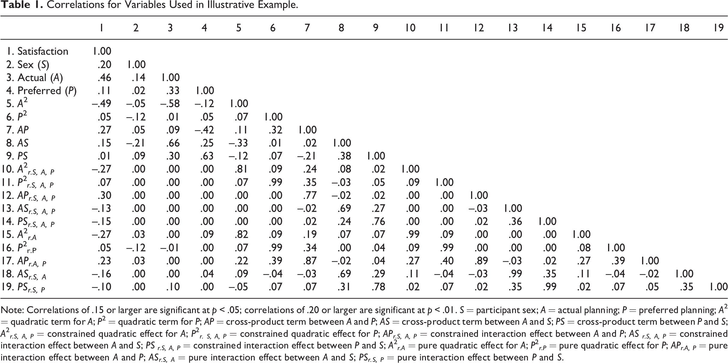
Note: Correlations of .15 or larger are significant at p < .05; correlations of .20 or larger are significant at p < .01. S = participant sex; A = actual planning; P = preferred planning; A² = quadratic term for A; P² = quadratic term for P; AP = cross-product term between A and P; AS = cross-product term between A and S; PS = cross-product term between P and S; A² _{r.S, A, P} = constrained quadratic effect for A; P² _{r. S, A, P} = constrained quadratic effect for P; AP_{r.S, A, P} = constrained interaction effect between A and P; AS _{r.S, A, P} = constrained interaction effect between A and S; PS _{r.S, A, P} = constrained interaction effect between P and S; A² _r.A = pure quadratic effect for A; P² _r.P = pure quadratic effect for P; AP_{r.A, P} = pure interaction effect between A and P; AS_{r.S, A} = pure interaction effect between A and S; PS_{r.S, P} = pure interaction effect between P and S.

Strategy 1—ΔR² and Hierarchical F Test (a between-sets test)

Table 2 contains a summary of the results for Strategy 1. As noted earlier, this strategy is most commonly used and optimally suited to tell us the relative contributions that different sets of variables make to the overall R². In this case, the R² for the first-order model (Model 1) was .235, the R² for the model adding the second-order quadratic terms (Model 2) was .317, and the R² for the model adding the second-order cross-product terms (Model 3) was .437. To estimate the relative contribution of sets of effects, one simply calculates the ΔR² values as one moves up the regression hierarchy. Specifically, we see that the relative contribution of the set of first-order (main) effects is .235, the relative contribution for the set of second-order quadratic effects is .082 (ΔR² = .317 – .235), and the relative contribution for the second-order interaction effects is .120 (ΔR² = .437 – .317). These results suggest that main effects are explaining the lion’s share of variance followed by the quadratics and interactions. Each of these increments was statistically significant, suggesting that at least one of the effects within each set of variables was likely statistically significant.

Table 2.

Results for Strategy 1 (between-sets test) and Strategy 2 (within-sets test) Using Illustrative Data From Edwards (1994).

							Strategy 1	Strategy 2
Model	Variable	B	SE of B	t	p	R ²	ΔR²	Constrained RW
Set 1: Main effects	Intercept	20.31	0.88	22.97	.000	.235*	.235*
	Sex (S)	2.35	1.18	1.99	.048			—
	Actual (A)	0.39	0.06	6.36	.000			—
	Preferred (P)	–0.05	0.08	–0.63	.532			—
Set 2: Main effects + quadratics	Intercept	21.60	1.09	19.81	.000	.317*	.082*
	Sex (S)	2.72	1.13	2.41	.017			—
	Actual (A)	0.21	0.07	2.95	.004			—
	Preferred (P)	–0.02	0.08	–0.31	.759			—
	A ²	–0.02	0.01	–4.35	.000			.076
	P ²	0.01	0.01	1.44	.152			.007
Set 3: Main effects + quadratics + interactions	Intercept	22.21	1.05	21.26	.000	.437*	.120*
	Sex (S)	1.96	1.17	1.68	.094			—
	Actual (A)	0.15	0.09	1.70	.092			—
	Preferred (P)	0.34	0.10	3.28	.001			—
	A ²	–0.03	0.01	–5.72	.000			—
	P ²	–0.00	0.01	–0.50	.616			—
	AP	0.04	0.01	5.16	.000			.092
	AS	–0.12	0.11	–1.10	.273			.010
	PS	–0.31	0.15	–2.06	.041			.018

Note: S = participant sex; A = actual planning; P = preferred planning; A² = quadratic term for A; P² = quadratic term for P; AP = cross-product term between A and P; AS = cross-product term between A and S; PS = cross-product term between P and S.

*p < .001 for R² and ΔR².

Examination of the t test on regression coefficients identifies those predictors that explain significant and unique (i.e., incremental) variance in satisfaction. These t tests reveal one of the shortcomings associated with a singular focus on significance testing among correlated predictors—which effects emerge as significant depends on which step in the hierarchy being examined. For example, Model 1 (the main effects model) suggests that preferred planning does not explain unique variance in satisfaction, but both participant sex and actual planning do explain such variance. In contrast, Model 3 (containing all effects) suggests the exact opposite: Participant sex and actual planning are not uniquely related to satisfaction, but preferred planning is uniquely related. Obviously, one must use caution when interpreting significant main effects in the presence of significant higher order effects. However, these results reveal the inherent limitation associated with a singular focus on significance testing. These “bouncing betas” are likely driven, at least in part, by collinearity among the main effects and between the main effects and higher order terms.

In summary, Strategy 1 provides us with a very nice big picture, between-sets view of our model. It tells us that each of the three sets of variables is contributing to our understanding of satisfaction in a unique way (i.e., the information in each set is not statistically redundant with the information contained in the other sets). The significance tests also permit us to understand the incremental effects of individual predictors, but not the overall or relative importance of these predictors and their effects. Indeed, as LeBreton et al. (2007) noted, “Relying solely on incremental validity may mask the practical contribution a . . . predictor makes to the R², when that predictor is correlated with some of the remaining predictors” (p. 488). Basically, small (and even nonsignificant) incremental effects may still be important (cf. Cortina & Landis, 2009; LeBreton et al., 2007), and these effects could be overlooked by relying solely on significance tests.

Strategy 2—Constrained Relative Importance Analysis (a within-set test)

Although Strategy 1 provides some useful information, that information is rather general as we are not able to distinguish the relative contribution of specific effects within the sets. For example, Strategy 1 does not let us determine the relative contribution of the various within-set quadratic effects to the overall explanatory power of the model. However, we can invoke Strategy 2 (constrained relative importance analysis) and compare the relative contribution of effects within specific subsets. This approach simply residualizes all higher order terms for all lower order terms. However, as noted earlier, within the context of interaction effects and polynomial effects, this procedure results in residualizing the higher order terms for both the proper and improper lower order effects. For example, the quadratic term corresponding to actual planning should be residualized only for the main effect of actual planning (i.e., A² _r.A ). However, in a constrained relative importance analysis this quadratic term is also (improperly) residualized for preferred planning and participant sex (i.e., A² _{r.A, P, S} ). This highly conservative residualization strategy represents an undesirable consequence of invoking the constrained relative importance procedure in the presence of higher order effects. With only a few main effect terms, the impact of this conservative residualization approach is likely limited (assuming these main effects are not highly correlated with the higher order terms). However, as more terms are added or the correlations between the superfluous terms and the higher order terms increase, we are likely to see the consequence of this over-residualization procedure.

We conducted a constrained RWA examining the relative contribution of the two quadratic terms contained in Model 2 in Table 2. Basically, we residualized both quadratic terms for the main effects of participant sex, preferred planning, and actual planning. Thus, each quadratic term was residualized for one relevant and two irrelevant lower order effects. We obtained constrained relative weights of .076 for the actual planning quadratic term and .007 for the preferred planning quadratic term. As expected, these two weights sum (within rounding error) to .082, which corresponds to the incremental variance for Model 2 (see Table 2). We then conducted a similar analysis for our third and final model, which contained the interaction terms. For this analysis, each of the interaction terms was residualized (constrained) for the three main effects and the two quadratic effects prior to running the RWA. We obtained a constrained relative weight of .092 for the interaction between actual planning and preferred planning, a weight of .010 for the interaction between actual planning and participant sex, and a weight of .018 for the interaction between preferred planning and participant sex (we obtained an identical set of weights using constrained DA). Summing the values, we obtain .120, which corresponds to the incremental variance associated with Model 3 (see Table 2).

In summary, Strategy 2 provides us with a more refined understanding of the relative contributions our higher order effects make within very specific subsets of predictors after first controlling for other predictors. As we moved up the hierarchy, we constrained (residualized) higher order terms for lower order terms. Doing so, we were able to see that the quadratic effect of actual planning and the actual planning by preferred planning interaction effect appeared to be quite important at driving the changes in R² at Steps 2 and 3 in our regression analysis. These results are consistent with the significance tests reported in Table 2. In addition, the constrained importance weights furnish supplemental information in the form of effect size estimates (i.e., proportion of variance in the ΔR² that should be attributed to each effect).

Strategy 3—Residualized Relative Importance Analysis (a between- and within-sets test)

Although the constrained RWA provided greater insight into the relative contribution of variables within a particular set of variables, it has two potential limitations. First, as noted earlier, this procedure may result in nebulous interpretations of importance when higher order effects are residualized for irrelevant lower order effects. Second, the purpose of the constrained analysis is to focus on relationships within a specific set of variables (e.g., the relationship among a set of quadratic terms); it does not furnish a simultaneous variance decomposition for all variables in the regression model. These two limitations can be avoided if the third strategy is used.

Our third strategy integrates and extends the information obtained from between-sets approach (Strategy 1) with the information obtained from a within-sets approach (Strategy 2). It also provides more appropriate estimates of the relative effect sizes because the higher order terms are residualized for only the relevant lower order terms. To illustrate this integration, we conducted a residualized relative importance analysis on all of the effects of interest in our regression model. Specifically, we calculated regression terms that were correctly residualized for only the appropriate lower order effects and then used these terms (which now correspond to the higher order effects) in a relative importance analysis. Results are presented in Table 3.

Table 3.

Results for Strategy 3 (residualized relative importance analysis: comprehensive within and between sets tests) Using Illustrative Data From Edwards (1994).

Predictor	Residualized Relative Importance Weight	Residualized Dominance Weight
Sex (S)	.028	.029
Actual (A)	.200	.202
Preferred (P)	.009	.008
A ² _r.A	.094	.093
P ² _r.P	.004	.003
AP_{r.A, P}	.075	.073
AS_{r.A, S}	.014	.016
PS_{r.P, S}	.013	.012

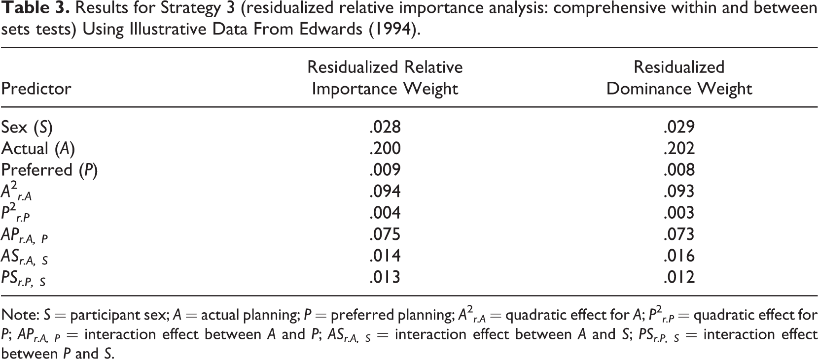
Note: S = participant sex; A = actual planning; P = preferred planning; A² _r.A = quadratic effect for A; P² _r.P = quadratic effect for P; AP_{r.A, P} = interaction effect between A and P; AS_{r.A, S} = interaction effect between A and S; PS_{r.P, S} = interaction effect between P and S.

This table provides a simultaneous comparison of main effects, quadratic effects, and interactions. There are several important conclusions to be drawn from this table. First, we are able to compare the relative importance of variables both within and between sets. For example, we are now able to directly compare the relative importance of the main effect for preferred planning to the quadratic effect of preferred planning. That is, we are able to fully interpret a comparison of the main effect and interaction effect of the same variable (e.g., preferred planning). However, such a comparison is possible only after the lower order effect (e.g., main effect) has been removed from the higher order term (e.g., cross-product term), thus yielding an estimate of the higher order effect (e.g., interaction effect). With ordinal interactions one would expect the main effects to typically trump the interactions, whereas in disordinal interactions we would expect the interaction effects to trump the main effects.

Second, we see that our estimates for the relative importance of the quadratic effects differed slightly from those obtained in Strategy 2, revealing the consequences of residualizing for improper terms. This is not surprising because Strategy 2 and Strategy 3 are partitioning different sources of variance (i.e., ΔR² associated with quadratics vs. total R² associated with all effects). Specifically, the results of a residualized RWA using Strategy 3 reveal the estimate for the quadratic effect of actual planning was .094 compared to the constrained quadratic effect of .076 obtained using Strategy 2. This absolute difference may seem small, but it represents a 24% difference associated with using Strategy 2 (i.e., [.094 – .076] / .076 = .237 × 100 = 24%). Again, we do not know all of the factors that give rise to such differences, and not all estimates necessarily will reveal large differences. However, it should be obvious that as the collinearity between the higher order terms and the irrelevant main effects increases, so too will the differences between estimates obtained using residualized relative importance analysis and constrained relative importance analysis.

Furthermore, Strategy 3 permits researchers to compare the relative impact of effects across or between sets. This helps them understand the extent to which the relationships hypothesized in their theories translate into actual effects. For example, we can compare the relative contribution of a specific main effect such as actual planning to its corresponding quadratic effect and the two-way interactive effects to which it contributed to determine if our hypotheses about these effects (and their relative importance) were supported. We can also compare this main effect directly to higher order effects to which it did not contribute (e.g., Preferred Planning × Participant Sex interaction effect). These comparisons help us understand the relative impact of these effects on the outcomes in a model that was derived from organizational theory. Thus, the relative effect sizes presented in Table 3 allow us to empirically test our theory (i.e., they tell us which effects are driving our model) and to better understand the results we obtained from the regression analysis presented in Table 2. For example, as we noted earlier, the main effect of preferred planning was inconsistent across the various models. Initially it was nonsignificant (see Model 1 in Table 2), but later emerged as significant in the final model (see Model 3 in Table 2). Although the regression weight is statistically different from zero (suggesting preferred planning is uniquely related to satisfaction), we see that the relative effect size associated with this predictor suggests a very tiny effect (relative weight = .009; see Table 3). So while testing a hypothesis concerning the significance of a predictor, it is also important to take into account not only statistical significance, but also effect size and context (Cortina & Landis, 2009; LeBreton et al., 2007).

In summary, we believe our third and final strategy provides information that many scholars may find useful. Specifically, by providing estimates of relative effect size, researchers are better able to integrate statistical significance with practical significance. In addition, because all of the weights contained in Table 3 sum to the model R², it is possible to calculate rescaled relative importance weights by dividing residualized relative importance weights by R². Such weights are interpreted as the percentage contribution of each effect to the overall predictive power of our model.

As we noted in the opening pages of our article, regression analysis has historically been used to estimate R² and significance tests on individual predictors. However, the statistical significance of individual regression coefficients does not always reflect the actual contribution a variable makes to the explanatory power of a regression model (Courville & Thompson, 2001). For example, LeBreton et al. (2007) noted that

[S]ignificance tests do not indicate the importance of predictor variables in a regression model. In fact, with large enough sample sizes, all incremental validity analyses and relative importance analyses will become statistically significant. Indeed, one of the advantages of a relative importance analysis is that it also furnishes estimates of importance scaled in the metric of relative effect sizes. . . . [T]his enables I-O psychologists to ascertain the practical importance of [predictor variables] without relying on sample-size-dependent significance tests. (p. 483)

Thus, we encourage researchers to continue examining the significance of their regression coefficients (which reveals incremental importance), but we also recommend that they examine the magnitude of relative importance weights (which reveals the relative effect sizes associated with particular effects). Researchers may also wish to use the procedures discussed in J. W. Johnson (2004) and Tonidandel, LeBreton, and Johnson (2009) to estimate the significance of relative weights or to compare whether two weights are different from one another.

Comparing and Contrasting Strategies

At this point it should be clear to the reader that different strategies partition variance differently and answer different research questions. Thus, there is not a single “correct” strategy to invoke when decomposing variance. Each approach has its strengths and limitations. For example, Strategy 1 is based on significance testing and thus aligns nicely with traditional interpretations of regression. Strategy 2 is well suited for situations containing control variables. It also uses the between-sets variance decomposition as its starting point. Thus, each separate within-set importance analysis will yield weights that sum to the between-sets ΔR²s. Finally, Strategy 3 is well suited for situations wherein the researcher wishes to residualize higher order terms only for the proper lower order effects. It is also useful for situations where a researcher wants to conduct a single, simultaneous variance decomposition. However, this approach, because it is based on only proper residualization, may yield weights that, if summed within sets, do not equal the ΔR²s. For example, summing the constrained relative importance weights yields a value of .082, corresponding to the ΔR² for Step 2 (see Table 2), whereas summing the residualized relative importance weights yields a value of .098 (i.e., .094 + .004 = .098). This difference stems from the residualization strategies invoked by these two procedures and the fact that the latter analysis simultaneously examines all higher order and lower order effects. Invoking a constrained analysis results in taking variance that was originally shared between the higher order effect and an irrelevant lower order effect and automatically crediting all of that variance to the irrelevant effect. In contrast, using the residualized analysis redistributes this shared variance, thus revealing that the quadratic effects are actually explaining slightly more variance than they are being credited using Strategies 1 or 2.

Limitations and Directions for Future Research

As one reviewer noted, measurement error will affect any strategy that relies on correlations or standardized regression coefficients. Thus, the results of all three strategies will be influenced by the level and pattern of measurement error in the predictors and criteria. To examine the impact of measurement error would necessitate a systematic examination probably via simulation. Unfortunately, such a simulation was well outside the scope of the current article. However, measurement error will affect correlations and regression coefficients, which form the basis of the strategies compared in our article (also see J. W. Johnson, 2004, for an illustration with respect to relative weights). Tonidandel and LeBreton (2011) noted that “the potential deleterious effects of measurement error on the observed relative importance indices could be compensated for by using a latent variable correlation matrix as input, rather than the observed correlation matrix” (p. 5). Clearly, additional research is needed in this area. In the current article, we simply assumed that variables were fixed and measured without error, which is the standard assumption underlying ordinary least squares regression (Cohen et al., 2003; Myers, 1990).

Related to the issue of measurement error is the issue of statistical significance. Ceteris paribus, as reliability increases one would expect to see more statistically significant effects because the observed effect sizes (correlations or regression coefficients) will increase. The reliability of higher order terms is in part a function of the product of the reliabilities of the lower order terms. Thus, as we test more sophisticated models, it is important to use highly reliable variables. Returning to our illustrative example, we find that the interaction effect for Actual Planning × Sex accounts for 3.2% of the R² but has a p value greater than .05. In contrast, the Preferred Planning × Sex interaction accounts for 2.9% of the variance but has a p value less than .05. How should we interpret such significance tests? Do we ignore the effect that explains more variance but that is nonsignificant, or do we look to the smaller but significant effect?

We suggest that any interpretation of an estimate of effect size should take into account the standard error of that measure and whether the confidence interval includes zero. However, collinearity should also be considered, so the statistical significance of a regression coefficient may not be the best indicator of whether one can account for a meaningful amount of variance. Instead, one should both interpret the magnitude of the relative weights themselves and also consider their confidence intervals. Specifically, one can determine whether those relative weights are significantly different from zero using a strategy similar to that recommended by Tonidandel et al. (2009). In the current article, we did not include a discussion of significance testing because those issues are tangential and have been presented elsewhere (see Tonidandel et al., 2009; Tonidandel & LeBreton, 2011).

Relative importance analyses share another basic assumption with ordinary least square regression analysis—namely, that the form and function of the regression model has been correctly specified (cf. Budescu, 1993; Tonidandel & LeBreton, 2011). Omitting relevant predictor variables will bias traditional regression weights, and it will also bias the results of relative importance analyses. However, to date, there has been limited work associated with model misspecification within the context of variable importance. Again, this is an area that would benefit from further systematic study.

One additional point that deserves comment is whether it is appropriate to combine the residualized relative importance weights for multiple effects associated with the same variable. It is our position that the higher order variables (which carry only the higher order effect) must be viewed as unique variables in the regression model and should not be combined with lower order variables. This is easily illustrated with an interaction effect. Specifically, a large relative importance weight for an interaction effect cannot be further decomposed into the importance of each of the two variables that compose that interaction effect. The same is also true of quadratics. For instance, the main effect, X, accounts for 5% of the variance and the quadratic effect, X² _r.X , accounts for 10% of the variance; it is not appropriate to say that the variable on the whole accounts for 15% of the variance. We believe such an interpretation is problematic for two reasons:

If we do combine importance weights of X and X² _r.X (10% + 5% = 15%), what will be a substantive interpretation of that combined effect? X and X² _r.X reflect different relationships between X and Y (a linear relationship and a curvilinear relationship, respectively), and a combination of their rescaled weights does not seem to be meaningful.

Combining the two effects would be especially problematic when X and X² _r.X are included in the model with an interaction effect (e.g., X by Z interaction), following Cortina’s recommendation. In this case, the interaction term will also contain the influence of X, and combining relative importance weights of only X and X² _r.X will not fully represent the role of X in the model predicting Y.

Nevertheless, this is an area that deserves further consideration and research. However, for the time being, we recommend that researchers refrain from aggregating multiple effects based on the same variable and instead report the variance explained by estimates for each individual effect.

Summary and Conclusion

Organizational researchers continue to be interested in using relative importance analyses to guide their interpretation of regression models. The ability to decompose the variance in criteria is instrumental to a comprehensive appreciation of which effects are driving the explanatory power of our models. With the first-order linear regression, such variance decompositions are readily addressed using a traditional relative importance analysis (e.g., DA, RWA). This is because, when examining an additive linear regression model, regression predictors are isomorphic with regression effects. That is, the U predictor carries with it only information about the U main effect. When running a relative importance analysis on the predictors in an additive linear regression, researchers are really seeking information about the relative importance of the effects of those predictors and, in an additive model, predictors equal effects.

However, as researchers develop more complicated models testing interactive and other higher order effects, alternative strategies for decomposing variance are needed. In the current article, we proposed three different strategies and discussed the types of inferences one can draw using these strategies. The final strategy, residualized relative importance, explicitly recognizes that higher order regression terms represent confounded, messy, and tainted variables that must be cleansed of the appropriate (i.e., relevant) lower order effects. This approach accomplishes three important things: (a) it creates a unique variable that equates predictors to effects (i.e., it creates an interaction term/variable equal to the interaction effect or nonlinear term/variable equal to the nonlinear effect), (b) it maintains the logic and mathematics of a hierarchical analysis, but in a separate step, “off-line,” when we compute the interaction or polynomial effect, and (c) it adjusts each higher order term for only the relevant lower order effects rather than adjusting those terms for all lower order effects, which is one of the potential limitations of Strategy 2—a constrained RWA.

By calculating the correct interaction term, we obtain an untainted assessment of the interaction effect. Creating this term is an “extra step” that is skipped when researchers use a traditional hierarchical regression. In the past, this extra step was unnecessary because researchers were simply interested in the statistical significance of the interaction effect (i.e., incremental importance)—and the hierarchical regression correctly estimated that significance. However, there is growing interest among researchers in supplementing basic questions about statistical significance (i.e., incremental importance) with follow-up questions about the relative contribution that predictors make to the overall explanatory power of the model (i.e., relative importance gauged in the metric of relative effect sizes; LeBreton et al., 2007). Thus, if we wish to draw inferences about the relative effect sizes of predictors and their effects, it is necessary that the correct predictors are included in the model and that they carry with them only the relevant statistical effects. The residualized relative importance approach accomplishes these goals and offers researchers a tool for comprehensively decomposing predicted variance in the higher order multiple regression models.

Footnotes

Appendix

Declaration of Conflicting Interests

The author(s) declared no potential conflicts of interest with respect to the research, authorship, and/or publication of this article.

Funding

The author(s) received no financial support for the research, authorship, and/or publication of this article.

Notes

References

Aguinis

(2004). Regression analysis for categorical moderators. New York, NY: Guilford.

Aguinis

Beaty

J. C.

Boik

R. J.

Pierce

C. A.

(2005). Effect size and power in assessing moderating effects of categorical variables using multiple regression: A 30-year review. Journal of Applied Psychology, 90, 94–107.

Aguinis

Pierce

C. A.

Bosco

F. A.

Muslin

I. S.

(2008). First decade of Organizational Research Methods: Trends in design, measurement, and data-analysis topics. Organizational Research Methods, 12, 69–112.

Aiken

L. S.

West

S. G.

(1991). Multiple regression: Testing and interpreting interactions. Newbury Park, CA: Sage.

Austin

J. T.

Scherbaum

C. A.

Mahlman

R. A.

(2002). History of research methods in industrial and organizational psychology: Measurement, design, analysis. In Rogelberg

S. G.

(Ed.), Handbook of research methods in industrial and organizational psychology (pp. 3–33). Malden, MA: Blackwell.

Azen

Budescu

D. V.

(2003). The dominance analysis approach for comparing predictors in multiple regression. Psychological Methods, 8, 129–148.

Bing

M. N.

LeBreton

J. M.

Davison

H. K.

Migetz

D. Z.

James

L. R.

(2007). Integrating implicit and explicit social cognitions for enhanced personality assessment: A general framework for choosing measurement and statistical methods. Organizational Research Methods, 10, 346–389.

Budescu

D. V.

(1993). Dominance analysis: A new approach to the problem of relative importance of predictors in multiple regression. Psychological Bulletin, 114, 542–551.

Budescu

D. V.

Azen

(2004). Beyond global measures of relative importance: Insights from dominance analysis. Organizational Research Methods, 7, 341–350.

10.

Casper

W. J.

Eby

L. T.

Bordeaux

Lockwood

Lambert

(2007). A review of research methods in IO/OB work-family research. Journal of Applied Psychology, 92, 28–43.

11.

Cohen

West

S. G.

Aiken

L. S.

(2003). Applied multiple regression/correlation analysis for the behavioral sciences (3rd ed.). Mahwah, NJ: Lawrence Erlbaum.

12.

Colquitt

J. A.

LePine

J. A.

Piccolo

R. F.

Zapata

C. P.

Rich

B. L.

(2012). Explaining the justice-performance relationship: Trust as exchange deepener or trust as uncertainty reducer. Journal of Applied Psychology, 97, 1–15.

13.

Cortina

J. M.

(1993). Interaction, nonlinearity, and multicollinearity: Implications for multiple regression. Journal of Management, 19, 915–922.

14.

Cortina

J. M.

Landis

R. S.

(2009). When small effect sizes tell a big story, and when large effect sizes don’t. In Lance

C. E.

Vandenberg

R. J.

(Eds.), Statistical and methodological myths and urban legends: Doctrine, verity and fable in the organizational and social sciences (pp. 287–308). New York, NY: Routledge.

15.

Courville

Thompson

(2001). Use of structure coefficients in published multiple regression articles: β is not enough. Educational and Psychological Measurement, 61, 229–248.

16.

Darlington

R. B.

(1968). Multiple regression in psychological research and practice. Psychological Bulletin, 69, 161–182.

17.

Eby

L. T.

Butts

Lockwood

(2003). Predictors of success in the era of the boundaryless career. Journal of Organizational Behavior, 24, 689–708.

18.

Edwards

J. R.

(1994). The study of congruence in organizational behavior research: Critique and proposed alternative. Organizational Behavior and Human Decision Processes, 58, 51–100.

19.

Edwards

J. R.

(2002). Alternatives to difference scores: Polynomial regression analysis and response surface methodology. In Drasgow

Schmitt

N. W.

(Eds.), Advances in measurement and data analysis (pp. 350–400). San Francisco, CA: Jossey-Bass.

20.

Edwards

J. R.

Parry

M. E.

(1993). On the use of polynomial regression equations as an alternative to difference scores in organizational research. Academy of Management Journal, 36, 1577–1613.

21.

Ganzach

(1997). Misleading interaction and curvilinear terms. Psychological Methods, 2, 235–247.

22.

Ganzach

(1998). Nonlinearity, multicollinearity and the probability of Type II error in detecting interaction. Journal of Management, 24, 615–622.

23.

Glomb

T. A.

Kammeyer-Mueller

J. D.

Rotundo

(2004). Emotional labor demands and compensating wage differentials. Journal of Applied Psychology, 89, 700–714.

24.

Jackson

C. L.

Colquitt

J. A.

Wesson

M. J.

Zapata-Phelan

C. P.

(2006). Psychological collectivism: A measurement validation and linkage to group member performance. Journal of Applied Psychology, 91, 884–899.

25.

James

L. R.

(1998). Measurement of personality via conditional reasoning. Organizational Research Methods, 1, 131–163.

26.

James

L. R.

Mulaik

S. A.

Brett

J. M.

(1982). Causal analysis: Assumptions, models, and data. Beverly Hills, CA: Sage.

27.

Johnson

J. W.

(2000). A heuristic method for estimating the relative weight of predictor variables in multiple regression. Multivariate Behavioral Research, 35, 1–19.

28.

Johnson

J. W.

(2001). The relative importance of task and contextual performance dimensions to supervisor judgments of overall performance. Journal of Applied Psychology, 86, 984–996.

29.

Johnson

J. W.

(2004). Factors affecting relative weights: The influence of sampling and measurement error. Organizational Research Methods, 7, 283–299.

30.

Johnson

J. W.

LeBreton

J. M.

(2004). History and use of relative importance indices in organizational research. Organizational Research Methods, 7, 238–257.

31.

Johnson

R. E.

Tolentino

A. L.

Rodopman

O. B.

Cho

(2010). We (sometimes) know not how we feel: Predicting job performance with an implicit measure of trait affectivity. Personnel Psychology, 63, 197–219.

32.

Krasikova

LeBreton

J. M.

Tonidandel

(2011). Estimating the relative importance of variables in multiple regression models. In Hodgkinson

G. P.

Ford

J. K.

(Eds.), International review of industrial and organizational psychology (pp. 119–141). Indianapolis, IN: John Wiley.

33.

LeBreton

J. M.

Binning

J. F.

Adorno

A. J.

Melcher

K. M.

(2004). Importance of personality and job-specific affect for predicting job attitudes and withdrawal behaviors. Organizational Research Methods, 7, 300–325.

34.

LeBreton

J. M.

Hargis

M. B.

Griepentrog

Oswald

F. L.

Ployhart

R. E.

(2007). A multidimensional approach for evaluating variables in organizational research and practice. Personnel Psychology, 60, 475–498.

35.

LeBreton

J. M.

Ployhart

R. E.

Ladd

R. T.

(2004). A Monte Carlo comparison of relative importance methodologies. Organizational Research Methods, 7, 258–282.

36.

LeBreton

J. M.

Tonidandel

(2008). Multivariate relative importance: Extending relative weight analysis to multivariate criterion spaces. Journal of Applied Psychology, 93, 329–345.

37.

Lievens

Conway

J. M.

De Corte

(2008). The relative importance of task, citizenship and counterproductive performance to job performance ratings: Do rater source and team-based culture matter? Journal of Occupational and Organizational Psychology, 81, 11–27.

38.

Lievens

Highhouse

De Corte

(2005). The importance of traits and abilities in supervisors’ hirability decisions as a function of method of assessment. Journal of Occupational and Organizational Psychology, 78, 453–470.

39.

Lindeman

R. H.

Merenda

P. F.

Gold

R. Z.

(1980). Introduction to bivariate and multivariate analysis. Glenview, IL: Scott, Foresman.

40.

Lubinski

Humphreys

L. G.

(1990). Assessing spurious “moderator effects”: Illustrated substantively with the hypothesized (“synergistic”) relation between spatial and mathematical ability. Psychological Bulletin, 107, 385–393.

41.

Luo

Y. D.

(2005). How important are shared perceptions of procedural justice in cooperative alliances? Academy of Management Journal, 48, 695–709.

42.

MacCallum

R. C.

Mar

C. M.

(1995). Distinguishing between moderator and quadratic effects in multiple regression. Psychological Bulletin, 118, 405–421.

43.

Martell

R. F.

Lane

D. M.

Emrich

(1996). Male-female differences: A computer simulation. American Psychologist, 51, 157–158.

44.

McAllister

D. J.

Kamdar

Morrison

E. W.

Turban

D. B.

(2007). Disentangling role perceptions: How perceived role breadth, discretion, instrumentality, and efficacy relate to helping and taking charge. Journal of Applied Psychology, 92, 1200–1211.

45.

Morgeson

F. P.

Nahrgang

J. D.

(2008). Same as it ever was: Recognizing stability in the BusinessWeek rankings. Academy of Management Learning and Education, 7, 26–41.

46.

Myers

R. H.

(1990). Classical and modern regression with applications (2nd ed.). Pacific Grove, CA: Brooks/Cole.

47.

Nickerson

Schwarz

Diener

Kahneman

(2003). Zeroing in on the dark side of the American dream: A closer look at the negative consequences of the goal for financial success. Psychological Science, 14, 531–536.

48.

Pedhazur

E. J.

(1997). Multiple regression in behavioral research: Explanation and prediction (3rd ed.). New York, NY: Harcourt Brace.

49.

Ployhart

R. E.

Hakel

M. D.

(1998). The substantive nature of performance variability: Predicting interindividual differences in intraindividual performance. Personnel Psychology, 51, 859–901.

50.

Podsakoff

P. M.

Dalton

D. R.

(1987). Research methodology in organizational studies. Journal of Management, 13, 419–441.

51.

Scandura

T. A.

Williams

E. A.

(2000). Research methodology in management: Current practices, trends, and implications for future research. Academy of Management Journal, 53, 1248–1264.

52.

Schleicher

D. J.

Venkataramani

Morgeson

F. P.

Campion

M. A.

(2006). So you didn’t get the job . . . now what do you think? Examining opportunity-to-perform fairness perceptions. Personnel Psychology, 59, 559–590.

53.

Shepperd

J. A.

(1991). Cautions in assessing spurious “moderator effects.” Psychological Bulletin, 110, 315–317.

54.

Stone-Romero

E. F.

Weaver

A. E.

Glenar

J. L.

(1995). Trends in research design and data analytic strategies in organizational research. Journal of Management, 21, 141–157.

55.

Tonidandel

LeBreton

J. M.

(2010). Determining the relative importance of predictors in logistic regression: An extension of relative weights analysis. Organizational Research Methods, 13, 767–781.

56.

Tonidandel

LeBreton

J. M.

(2011). Relative importance analysis: A useful supplement to regression analysis. Journal of Business and Psychology, 26, 1–9.

57.

Tonidandel

LeBreton

J. M.

Johnson

J. W.

(2009). Statistical significance tests for relative weights. Psychological Methods, 14, 387–399.

58.

Van Iddekinge

C. H.

Ployhart

R. E.

(2008). Developments in the criterion-related validation of selection procedures: A critical review and recommendations for practice. Personnel Psychology, 61, 871–925.

59.

Williams

E. J.

(1978). Linear hypotheses: Regression. In Kruskal

W. H.

Tanur

J. M.

(Eds.), International encyclopedia of statistics (pp. 523–541). New York, NY: Free Press.

Residualized Relative Importance Analysis

Abstract

Keywords

Decomposing Variance in the First-Order Multiple Linear Regression

General Dominance Weights

Relative Weights

Estimating and Testing Interactive and Other Higher Order Effects

Three Strategies for Decomposing the Variance Predicted by Main, Interactive, and Other Polynomial Effects in Higher Order Multiple Regression Models

Strategy 1—ΔR2 and Hierarchical F Test (a between-sets test)

Strategy 2—Constrained Relative Importance Analysis (a within-set test)

Strategy 3—Residualized Relative Importance Analysis (a between- and within-sets test)

Illustrative Example

Sample

Strategy 1—ΔR2 and Hierarchical F Test (a between-sets test)

Strategy 2—Constrained Relative Importance Analysis (a within-set test)

Strategy 3—Residualized Relative Importance Analysis (a between- and within-sets test)

Comparing and Contrasting Strategies

Limitations and Directions for Future Research

Summary and Conclusion

Footnotes

Appendix

Declaration of Conflicting Interests

Funding

Notes

References

Strategy 1—ΔR² and Hierarchical F Test (a between-sets test)

Strategy 1—ΔR² and Hierarchical F Test (a between-sets test)