Understanding the Results of Multiple Linear Regression

Abstract

Multiple linear regression (MLR) remains a mainstay analysis in organizational research, yet intercorrelations between predictors (multicollinearity) undermine the interpretation of MLR weights in terms of predictor contributions to the criterion. Alternative indices include validity coefficients, structure coefficients, product measures, relative weights, all-possible-subsets regression, dominance weights, and commonality coefficients. This article reviews these indices, and uniquely, it offers freely available software that (a) computes and compares all of these indices with one another, (b) computes associated bootstrapped confidence intervals, and (c) does so for any number of predictors so long as the correlation matrix is positive definite. Other available software is limited in all of these respects. We invite researchers to use this software to increase their insights when applying MLR to a data set. Avenues for future research and application are discussed.

Keywords

multiple regression quantitative research exploratory research design

A continued goal of organizational researchers conducting regression analysis is to make inferences about the relative importance of predictor variables (cf. Nimon, Gavrilova, & Roberts, 2010; Zientek, Capraro, & Capraro, 2008), yet it is all too common to rely heavily (if not solely) on the regression coefficients from the analysis which optimize sample-specific prediction (minimize sum of squared errors). Instead, other metrics that operationalize relative importance in ways that are consistent with such researchers’ goals would seem more appropriate, and a range of metrics and approaches exists. In addition to regression weights and zero-order correlation coefficients that researchers likely report, MLR interpretation may be further informed by considering structure coefficients, product measures, relative weights, all-possible-subsets regression, dominance weights, and commonality coefficients. The current article offers software that cogently summarizes these metrics so that researchers can make more sophisticated judgments about the nature and meaningfulness of variables in a linear regression model than judgments from regression weights or any single metric in isolation. As noted by Nathans, Oswald, and Nimon (2012), each metric serves a different purpose and has certain features that support interpreting specific aspects of a multiple linear regression (MLR) model (see Table 1).

Table 1.

Regression Metric/Analysis and Their Associated Purpose and Features.

Regression Metric/Analysis	Purpose	Variable Importance^a	Partition R²	Identify Presence of Multicollinearity and Suppression?
Regression weight	Identifies contribution of each IV to the regression equation, holding all other IVs constant	Total	Into p partitions, with standardized data and uncorrelated IVs	With zero-order correlation or structure coefficients
Zero-order correlation coefficient	Identifies magnitude and direction of the relationship between the IV and DV, without considering any other IVs in the MLR model	Direct	Into p partitions, when squared and with uncorrelated IVs	With regression weights
Squared structure coefficient	Identifies how much variance in the predicted scores ( $\hat{Y}$ ) for the DV can be attributed to each IV	Direct	Into p partitions, with uncorrelated IVs	With regression weights and when summed and compared to unity
Pratt measure	Partitions the regression effect into nonoverlapping partitions based on multiplying the beta weight of each independent variable with its respective zero-order correlation with the dependent variable	Direct and total	Into p partitions	May identify presence of multicollinearity or suppression
Relative weight	Determines how IVs contribute to the DV when expressed as a joint function of (a) how highly related IVs are to their uncorrelated counterpart and (b) how highly related the uncorrelated counterparts relate to the DV	Total	Into p partitions	Do not identify presence of multicollinearity or suppression
All-possible-subsets regression	Determines the R² for MLRs from all possible 2 ^p –1 subsets of IVs; serves as base for commonality and dominance analysis	N/A	N/A	May identify presence of multicollinearity or suppression
Commonality analysis	Identifies how much variance in the DV is uniquely explained by each possible IV set in the MLR; yields unique and common effects that, respectively, identify variance unique to one IV and multiple IVs	Total	Into 2 ^p –1 partitions.	Identify presence, location, and magnitude of multicollinearity and suppression
Dominance analysis	Indicates whether one IV contributes more unique variance than another IV, either (a) across all possible MLR submodels (i.e., complete dominance) or (b) on average across models of all-possible-subset sizes (i.e., conditional dominance); averaging conditional dominance weights yields general dominance weights	Direct, total, and partial	Into p partitions with general dominance weights	Conditional dominance weights may identify presence of suppression

Note: Adapted from Nathans, Oswald, and Nimon (2012). p = number of predictor; IV = independent variable; DV = dependent variable; MLR = multiple linear regression.

^aQuantifies IV importance when: (a) measured in isolation from other IVs (direct effect), (b) contributions of all other IVs have been accounted for (total effect), and (c) contributions to regression models of a specific subset or subsets of other IVs have been accounted for (partial effect). See Nathans et al. (2012) for more on advantages, disadvantages, and recommendations for practice.

The aforementioned metrics are reviewed here briefly, but for more details we refer the reader to other work, both recent and historical in nature (e.g., Budescu, 1993; Darlington, 1968; Johnson, 2000; Johnson & LeBreton, 2004; Kraha, Turner, Nimon, Zientek, & Henson, 2012; Krasikova, LeBreton, & Tonidandel, 2011; Lindeman, Merenda, & Gold, 1980; Tonidandel & LeBreton, 2011). This allows the current article to take a more practical focus on the software tool and its capabilities, with the support of two empirical examples.

Regression Weights

In MLR models, raw data yield unstandardized (raw) regression weights, and standardized data yield standardized regression weights. Regardless of whether or not the data are standardized, the values residing in the vector b = $(b_{1}, b_{2}, b_{3}, \dots b_{p})$ are chosen in such a way that the weighted composite $b^{T} X$ is maximally correlated with the dependent variable, Y, which is external to the composite (i.e., choose b so that r[ $b^{T} X$ , Y ] is maximized). This is the same as choosing b to minimize the variance of the errors in prediction (i.e., choose b so that $[v a r (Y) - b^{T} R_{X X} b]$ is minimized). If we assume that we are using standardized regression coefficients, then each coefficient b_k indicates the expected change in Y, in standard deviation units, given a corresponding 1 standard deviation change in X_k , when all the other predictors in the model in X (i.e., $(X_{1}, X_{2}, \dots X_{k - 1}, X_{k + 1}, \dots X_{p})^{T}$ ] are fixed or controlled for.

It may be reasonable to assume that predictors with larger standardized coefficients (called betas henceforth) are more important than other predictors with smaller coefficients. Certainly this is true when variables are uncorrelated, because in that case, betas are exactly equal to the zero-order correlations between X and Y . However, when the predictors in X are correlated, standardizing does not disentangle the effects of X on Y from the standard deviations of X ; in fact, it confounds them in the service of placing all weights on a z-score metric.

Zero-Order Correlation Coefficients

Obviously, prediction of Y from each independent variable X_i is found in R_XY , the vector of zero-order correlation coefficients (often called validity coefficients). If all variables in X were completely uncorrelated (i.e., R_XX = I, the p × p identity matrix), then the contribution of each X_i to Y can be clearly represented as the squared values in R_XY , because these squared values are independent of one another, meaning that they partition R² or, equivalently, they add up to the model R² (i.e., $R_{X Y}^{^{'}} R_{X Y}$ = R²). However, when predictors are correlated, the sum of the elements in $r_{X Y}^{2}$ will not add up to the model R², necessitating other metrics to determine how the MLR model is affected by multicollinearity.

Structure Coefficients

One relatively simple approach to determining the contribution of p independent variables in linear regression is through calculating a p × 1 vector of structure coefficients ( sr ), which are the correlations between each predictor X and $\hat{Y}$ , the latter being the predicted values of Y . Equivalently, structure coefficients can be calculated by dividing the p × 1 vector of zero-order validity coefficients $R_{X Y}$ by the multiple R; thus,

s r = \frac{R_{X Y}}{\sqrt{b^{T} R_{X Y}}} = \frac{R_{X Y}}{R} = r_{X \hat{Y}} .

Structure coefficients have been used to indicate the relative contributions of each X_i to the prediction of Y, but they cannot be interpreted in a straightforward manner when variables in X are correlated or when there are suppression effects (i.e., the sum of the elements in ${r^{2}}_{X \hat{Y}}$ does not equal unity).

Pratt Measure

The Pratt measure, or product measure, of a predictor variable’s relative importance was proposed by Pratt (1987) and is defined simply as $m_{i} = b_{Y X_{i}} r_{Y X_{i}}$ : the product of the standardized regression coefficient and the zero-order validity coefficient for X_i . Pratt measures divide the model R ²across predictor variables, meaning that

R^{2} = b^{T} R_{X Y} = \sum_{i = 1}^{p} m_{i},

where each component of the sum is a Pratt measure ( $m_{i}$ ). The Pratt measure can be viewed as problematic in cases where individual values are negative or zero values, because those might be products of suppression or multicollinearity that require further explanation (see Thomas, Hughes, & Zumbo, 1998). However, this decomposition remains in the literature as a common method for decomposing R², and we include it in our software package, if only to compare it with more modern methods such as general dominance and relative weights.

Relative Weights

Relative weights are another way to partition an MLR model R² across predictors. They are computed by first transforming p predictors into a new set of p variables that are uncorrelated with one another, yet are correlated as highly as possible with the original predictors; that is, given the data matrix $X = P Δ Q^{T}$ , then create the new variables $Z = P Q^{T}$ . Fabbris (1980) noted that treating X as a set of dependent variables and regressing X onto Z creates M , the p × p correlation matrix between the original predictors and their orthogonal counterparts; this was rediscovered by Genizi (1993) and then in the organizational literature by Johnson (2000). It may be somewhat surprising to know that M is also equal to the matrix square root of the predictor intercorrelation matrix ( $M = {(Z^{'} Z)}^{- 1} Z^{T} X = Z^{T} X = Q Δ Q^{T} = R_{x x}^{1 / 2}$ ). Also surprising might be that the squared elements in each column (or each row) of M (or $R_{x x}^{1 / 2}$ ) sum to 1.

These elements for each column are used to weight each predictor variable according to its independence from other predictor variables (i.e., a higher weight will mean greater independence from that variable). In addition to this matrix, regressing Y on Z yields a p × 1 vector of orthogonal weights we call V (i.e., $V = {(Z' Z)}^{- 1} Z^{T} y = Z^{T} y$ ∫). Because the components of Z are uncorrelated and all variables are standardized, the squared values in $V$ also sum to 1, where each element provides the proportional contribution of each orthogonalized predictor Z_i to Y .

Thus, a relative weight multiplies or “glues” like elements from the two orthogonal vectors of M and V weights just described, namely, (a) the ith squared regression weight for the given predictor regressed onto its orthogonal counterpart multiplied by (b) the ith squared weight regressing the criterion on that given predictor’s orthogonal counterpart. Mathematically, the relative weight for predictor i is called $ϵ_{i}^{2}$ and equals

ϵ_{i}^{2} = \sum_{j = 1}^{p} \{M_{i j}^{2} V_{j}^{2}\},

and each of the p relative weights across is an independent part of the total model R², meaning the weights add to R² ( $R^{2} = \sum_{i = 1}^{p} ϵ_{i}^{2}$ ) even when the independent variables are correlated (see Fabbris, 1980; Genizi, 1993; Johnson, 2000). In this way, relative weights are easy to explain in the same way as general dominance weights because they sum to the model R². Alternatively, the relative weights can be re-expressed as proportions or percentages of R².

Relative weights are thus defined as the contribution of a given predictor to criterion variance, considering the predictor’s contribution alone as well as jointly with the other predictors in the model. Note that relative weights and general dominance weights have often been found to rank predictors similarly in terms of relative importance (Johnson, 2000); however, the current software program can verify where results converge or diverge.

All-Possible-Subsets Regression

As the name implies, all-possible-subsets (APS) regression involves running linear regression models on all 2 ^p – 1 subsets of predictors. In doing so, one often takes either a predictor-based approach or model-based approach to the set of results. APS is best compared to other metrics when taking a predictor-based approach, where a predictor deemed more important within a regression model will tend be one that is more important across submodels in APS regression. APS regressions can be analyzed in this manner for each predictor, or one can use commonality coefficients or dominance weights, to be discussed next, because these are based on the results of APS regressions.

In addition to the predictor-based approach, researchers and practitioners also may take a model-based approach to APS, because it is an exploratory approach to determining the tradeoff between model parsimony and model fit, where a submodel with fewer predictors retains a model R² that is either similar to the full model R² or is above some practical minimum established by the researcher or practitioner. Obviously, the model-based approach can be related to the variable-based approach when there is a consistent recommendation to include and/or exclude specific predictors across models.

Commonality Analysis

Commonality analysis partitions the R² explained by all predictors in multiple regression into variance unique to each predictor and variance shared between each combination of predictors (see Mayeske et al., 1969; Mood, 1969, 1971; Newton & Spurrell, 1967; Onwuegbuzie & Daniel, 2003; Rowell, 1996). These components of variance are called commonality coefficients that can then be evaluated in terms of their magnitude, and they can be compared with one another. As partitions, commonality coefficients sum to the total R² for the regression model.

There are two general types of commonality coefficients: unique effects and common effects. The unique effect of a predictor (also called the uniqueness coefficient) is the square of the semipartial correlation between a given predictor and the criterion. Thus, if predictors are all uncorrelated, then predictor importance can be entirely determined by ranking the unique effects. When predictors are correlated, as is usually the case, the common effects can indicate the extent and pattern of the predictors’ shared variance in predicting variance in the criterion (Mood, 1971).

Consider the hypothetical situation discussed by Hedges and Olkin (1981) in which two variables, X1 and X2, are used to predict a variable X0. For this regression equation, the explained variance (R² _0.12) can be partitioned into three components:

γ_{1} {= u n i q u e c o n t r i b u t i o n o f X 1 t o R}_{0 .12}^{2},

γ_{2} {= u n i q u e c o n t r i b u t i o n o f X 2 t o R}_{0 .12}^{2},

γ_{12} = c o m m o n c o n t r i b u t i o n o f X 1 a n d X 2 t o R_{0.12}^{2},

and they are computed as follows:

γ_{1} = R_{0.12}^{2} - R_{0.2}^{2},

γ_{2} = R_{0.12}^{2} - R_{0.1}^{2},

γ_{12} = R_{0.1}^{2} + R_{0.2}^{2} - R_{0.12}^{2} .

Commonality coefficients provide researchers with rich detail about how independent variables operate together in a given regression model. The coefficients are more specific than regression weights, relative weights, or general dominance weights. As Seibold and McPhee (1979) noted, “[Only by] determining the extent to which…independent variables, singly and in all combinations, share variance with the dependent variable…can we fully know the relative importance of independent variables with regard to the dependent variable in question” (p. 355).

Note that negative values of commonality coefficients generally indicate that a predictor exerts a suppressor effect, where it is removing (partialing out) the irrelevant variance in the other predictor(s) to increase the latter’s contributions to the model R² (Zientek & Thompson, 2006). Unlike other metrics, commonality coefficients are uniquely able to pinpoint the predictors involved in a suppressor relationship and the specific nature of that relationship. Summing all negative common effects for a regression equation can quantify the amount of suppression present in the regression model as a whole.

Dominance Analysis

A regression metric was originally proposed by Chevan and Sutherland (1991), then elaborated upon by Budescu (1993), who detailed the procedure for conducting a dominance analysis. Dominance analysis involves computing each predictor’s incremental validity across all possible submodels that involve that predictor and using the incremental validity coefficients to evaluate complete dominance, conditional dominance, and general dominance. To make the dominance analysis procedure more concrete, see the dominance analysis formulas in Table 2 that support a three-predictor MLR model.

Table 2.

Dominance Analysis Formulas for Three Predictor Case.

		Additional Contribution of:
Subset Model (X)	$R_{Y . X}^{2}$	X1	X2	X3
CD, k = 0 average		$R_{Y . X 1}^{2}$	$R_{Y . X 2}^{2}$	$R_{Y . X 3}^{2}$
X1	$R_{Y . X 1}^{2}$		$R_{Y . X 1 X 2}^{2} - R_{Y . X 1}^{2}$	$R_{Y . X 1 X 3}^{2} - R_{Y . X 1}^{2}$
X2	$R_{Y . X 2}^{2}$	$R_{Y . X 1 X 2}^{2} - R_{Y . X 2}^{2}$		$R_{Y . X 2 X 3}^{2} - R_{Y . X 2}^{2}$
X3	$R_{Y . X 3}^{2}$	$R_{Y . X 1 X 3}^{2} - R_{Y . X 3}^{2}$	$R_{Y . X 2 X 3}^{2} - R_{Y . X 3}^{2}$
CD, k = 1 average		$\frac{(R_{Y . X 1 X 2}^{2} - R_{Y . X 2}^{2}) + (R_{Y . X 1 X 3}^{2} - R_{Y . X 3}^{2})}{2}$	$\frac{(R_{Y . X 1 X 2}^{2} - R_{Y . X 1}^{2}) + (R_{Y . X 2 X 3}^{2} - R_{Y . X 3}^{2})}{2}$	$\frac{(R_{Y . X 1 X 3}^{2} - R_{Y . X 1}^{2}) + (R_{Y . X 2 X 3}^{2} - R_{Y . X 2}^{2})}{2}$
X1X2	$R_{Y . X 1 X 2}^{2}$			$R_{Y . X 1 X 2 X 3}^{2} - R_{Y . X 1 X 2}^{2}$
X1X3	$R_{Y . X 1 X 3}^{2}$		$R_{Y . X 1 X 2 X 3}^{2} - R_{Y . X 1 X 3}^{2}$
X2X3	$R_{Y . X 2 X 3}^{2}$	$R_{Y . X 1 X 2 X 3}^{2} - R_{Y . X 2 X 3}^{2}$
CD, k = 2 average		$R_{Y . X 1 X 2 X 3}^{2} - R_{Y . X 2 X 3}^{2}$	$R_{Y . X 1 X 2 X 3}^{2} - R_{Y . X 1 X 3}^{2}$	$R_{Y . X 1 X 2 X 3}^{2} - R_{Y . X 1 X 2}^{2}$
X1X2X3	$R_{Y . X 1 X 2 X 3}^{2}$
GD, overall average		$\frac{\sum_{k = 0}^{2} C D_{X 1}}{3}$	$\frac{\sum_{k = 0}^{2} C D_{X 2}}{3}$	$\frac{\sum_{k = 0}^{2} C D_{X 3}}{3}$

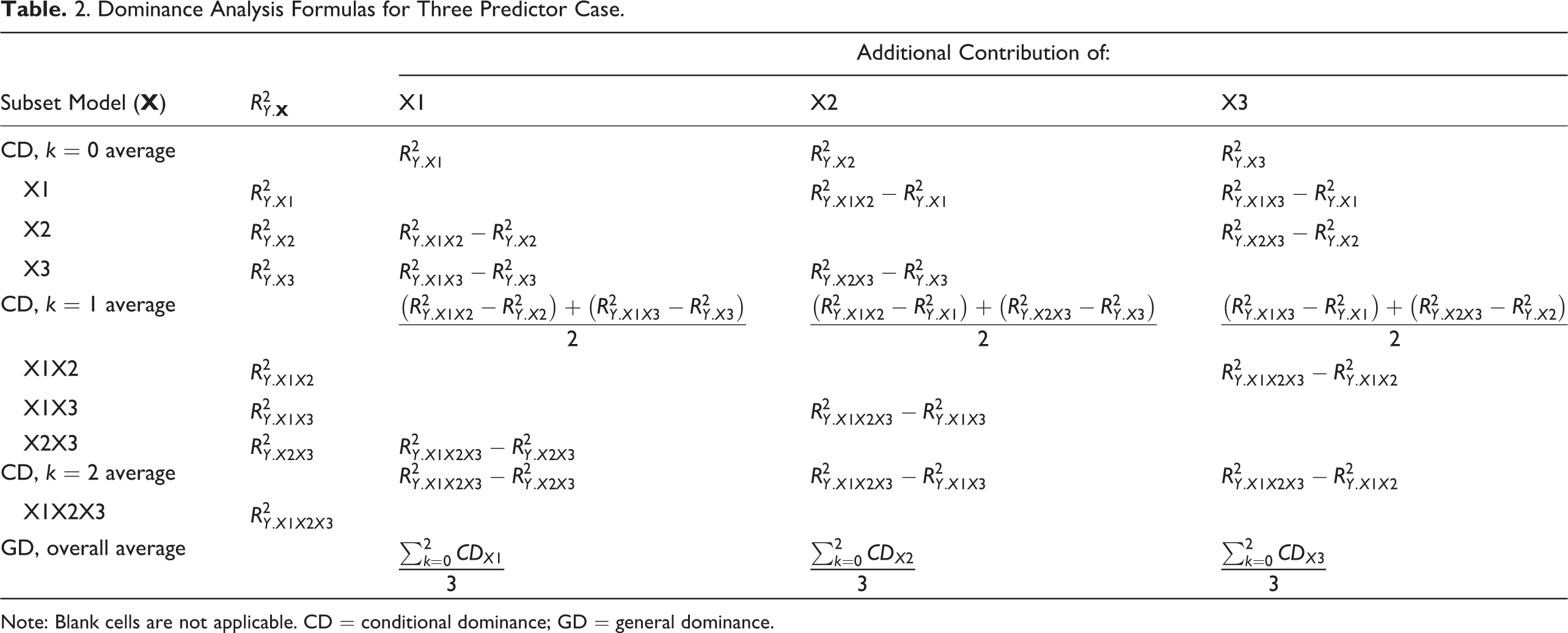
Note: Blank cells are not applicable. CD = conditional dominance; GD = general dominance.

If incremental validity is always higher for X_i than for X_j for every submodel, then X_i is said to show complete dominance over X_j . Complete dominance is a restricted form of dominance that may rarely occur. There is a more relaxed form of dominance called conditional dominance, which occurs when the average incremental variance within each submodel of sizes 0 to p − 1 is greater for one predictor than another across all model sizes. The average incremental variance components used to evaluate conditional dominance are called conditional dominance weights. Conditional dominance weights are averaged across p predictors to create general dominance weights that partition the model R² across predictors. A predictor is said to show general dominance if it has the highest overall average incremental validity across regression submodels of sizes 0 to p − 1.

Dominance weights have two appealing properties: First, like relative weights, each general dominance weight is the average contribution of a predictor to a criterion, both on its own and when taking all other predictors in the model into account. Second, general dominance weights always sum to the overall model R². Third, conditional dominance weights have the potential to illuminate the properties of model predictors that can get lost in commonality coefficients (which are numerous and can be difficult to interpret even when p = 3) or averaged away in more general metrics (e.g., relative weights, general dominance weights).

Software for Exploring the Predictor Space

The software tool we introduce was developed in R (R Development Core Team, 2013), and it offers a number of incremental contributions over both the literature and applications of the past addressing this topic of the relative importance of variables in linear regression analysis. First and most importantly, the software analyzes a wide variety of regression metrics within a single program. Recently, researchers have developed and provided computer programs, macros, and software packages to compute the metrics in linear regression to be discussed here, such as dominance analysis (Azen & Budescu, 2003) and relative weights (Grömping, 2006; Tonidandel, LeBreton, & Johnson, 2009). Although other researchers have integrated multiple metrics into their programs (Braun & Oswald, 2011), the current software is much more comprehensive in integrating all regression metrics reviewed here. Second, the software allows for some computational efficiencies; for instance, all-possible-subsets regression is computed and applied to multiple metrics rather than having to be computed each time within different programs. Third, the software computes confidence intervals (CIs) for all coefficients and for differences between specific pairs of coefficients. Confidence intervals are based on bootstrapping procedures and estimate an interval that 95% of the time, for example, contains the corresponding population parameter. Although this has been accomplished for some metrics (e.g., Algina, Keselman, & Penfield, 2010, for squared semipartial correlations; Lorenzo-Seva, Ferrando, & Chico, 2010, for bootstrapped regression coefficients, structure coefficients, and relative importance weights; and Tonidandel & LeBreton at the website http://relativeimportance.davidson.edu/ for bootstrapped relative importance weights in regression, multivariate regression [regression with multiple criteria], and logistic regression), this has not been accomplished to date across such a wide array of metrics within a more integrated software package as we have done here. To conduct statistical significance tests of metrics such as relative weights and general dominance weights, as in Tonidandel et al. (2009), one can include a randomly generated variable as an additional predictor in the model. This software will then automatically generate CIs on the differences between each predictor metric and the metric associated with the randomly generated variable, which can then be used to assess statistical significance. Our software program also graphs CIs, keeping in mind that the statistical differences between statistics may still be significant even when their respective CIs overlap (Cumming & Finch, 2005). Fourth, some software solutions have limited the number of predictors that are allowed; by contrast, our software computes metrics for as many predictors as are allowed by computer memory, by the positive definiteness of the predictor correlation matrix, and by the patience of the user. Fifth and finally, the software is available in R code, meaning that it is free to use, and anyone can read, learn from, revise, and extend the program code.

Method

We developed software to compute and bootstrap the regression metrics reviewed in this article, using R as our underlying platform. R is a “cutting-edge, free, open source statistical package” that runs on all commonly used operating systems (see R Development Core Team, 2013) and is gaining popularity across research disciplines (Culpepper & Aguinis, 2011). One major benefit of R platform is the opportunity for researchers to develop and update programs or “packages” to the R repository that extend the functions of the base system. To date, the R platform is supported by 4,461 user-contributed packages.

Extending the work of one of the user-contributed packages, yhat (Nimon & Roberts, 2012), the current article presents software that (a) calculates all of the regression results discussed in this article (calc.yhat), (b) bootstraps the results (boot.yhat), (c) evaluates the bootstrapped results (booteval.yhat), and (d) plots relevant CIs (plotCI.yhat). These extensions are reviewed in the sections that follow. We believe they represent a meaningful update to the yhat package.

calc.yhat

The calc.yhat function produces four sets of regression metrics. The first set is called PredictorMetrics and contains the predictor metrics reviewed in this article: b weights, beta weights, validity coefficients, structure coefficients, squared structure coefficients, unique coefficients, the sum of common coefficients, conditional dominance weights, general dominance weights, product measures, and relative weights.

The second set is called OrderedPredictorMetrics, and for each metric simply ranks the absolute values of the values contained in the PredictorMetrics set.

The third set is called PairedDominanceMetrics and contains the complete, conditional, and general dominance values (D_ij ) for each pair of predictors. As in Azen and Budescu (2003), a value of 1 in D_ij indicates that X_i dominates X_j , 0 indicates that X_j dominates X_i , and .5 indicates that dominance cannot be established between X_i and X_j .

The fourth set is called APSRelatedMetrics and contains commonality coefficients, which is the criterion variance partitioned across all subsets of independent variables. Also included are the multiple R²s resulting from an APS regression and the incremental variance for each predictor (the latter of which is used with uniqueness coefficients to determine general, conditional, and complete dominance).

boot.yhat

The boot.yhat function is based on the R package boot (Canty & Ripley, 2011) and supports the bootstrapping of all the metrics computed by calc.yhat. This function also computes a Kendall’s tau correlation for each type of predictor metric (e.g., r, β, r_s ), correlating bootstrap metrics with sample metrics to indicate stability of the ranking of each type of predictor metric, where high correlations imply agreement in the rank ordering. This feature would most likely be used to correlate the rank order of predictor metrics between like sample and bootstrap statistics. However, it is also possible for the user to pass a set of statistics such that each set of bootstrap statistics is correlated to the same set of sample statistics, as in LeBreton, Ployhart, and Ladd (2004), where the rank order of predictors from general dominance analysis was correlated with the rank order of predictors generated from alternative methods (e.g., product measure, R², relative weights analysis).

booteval.yhat

The booteval.yhat function takes the boot.yhat output generated across bootstrap iterations and calculates descriptive statistics and CIs based on them. Bootstrapped CIs avoid the need to rely on multivariate normality assumptions in the data or in the statistics generated from them. The accelerated bootstrap interval (“bca”) is the default CI. The basic bootstrap interval (“basic”), the accelerated bootstrap interval (“bca”), the first order normal approximation (“norm”), and the bootstrap percentile interval (“perc”) are also supported.

Descriptive Statistics

Regarding descriptive statistics, booteval.yhat produces tauDS, which contains the M and SD of Kendall’s tau (described earlier) across bootstrap iterations from boot.yhat. These results indicate how consistent the observed predictor ordering is between each bootstrapped sample and the actual sample (high mean and low variance indicates a consistent ordering). Also, for each pair of predictors, the M and SE of D_ij for each type of dominance is reported alongside the proportion of D_ij = 1 (P _ij), D_ij = 0 (P _ij), and D_ij = .5 (P _noij) across bootstrap replications, as well as the reproducibility of D_ij (Reprod).These values are in keeping with Azen and Budescu (2003). The SE of (D_ij ) = $\sqrt{\frac{1}{S - 1} \sum_{s = 1}^{S} (D_{i j}^{s} - {\overline{D}}_{i j})}$ , where S equals the number of bootstrap samples and the reproducibility of D_ij is the “proportion of bootstrap samples that agree with the sample results” (p. 141).

Confidence Intervals

For data in the PredictorMetrics and APSRelatedMetrics object, CIs are provided alongside and apart from sample statistics in objects, respectively, named combCIpm, lowerCIpm, upperCIpm and combCIaps, lowerCIaps, upperCIaps. The data in these objects allow researchers to make confidence statements regarding the associated metrics and to identify whether pairs of metrics differ to a statistically significant degree (i.e., the related CIs do not overlap).

However, when comparing the metric of one variable to another, overlapping CIs do not necessarily indicate a statistically nonsignificant difference between parameter estimates (see Cumming & Finch, 2001; Zientek, Yetkiner, & Thompson, 2010). One has to examine the distribution of differences between the two bootstrapped estimates of interest across replications. To that end, booteval.yhat also provides CIs around differences between select pairs of metrics. Confidence intervals around differences between pairs of predictors for each predictor metric are reported with sample statistics in combCIpmDiff and separately in lowerCIpmDiff and upperCIpmDiff. For each order of predictor combinations (e.g., 1st order, 2nd order,…kth order, where k = number of predictors), CIs around pairs of APS and commonality coefficients are reported with sample statistics in combCIapsDiff and separately in lowerCIapsDiff and upperCIapsDiff. Data in these objects allow researchers to determine whether the R²s or the commonality coefficients associated with a particular number of predictors are statistically significantly different from one another, which may be useful for identifying equivalent fitting models for a particular number of predictors (cf. Thompson, 2006) and for statistically evaluating the difference between joint variance components (cf. Schoen, DeSimone, & James, 2011). For each pair of predictors, CIs around differences between incremental variance are reported with sample statistics in combCIincDiff and separately in lowerCIincDiff and upperCIincDiff. Data in these objects provide insight into the determination of complete dominance across bootstrapped samples.

plotCI.yhat

The plotCI.yhat function plots the sample statistics and the upper and lower CI for associated objects that are passed to it, such as the sample statistics in PredictorMetrics. The function could also be used to plot the CI around sample statistics in APSRelatedMetrics when the number of predictors is small.

Other Functions

Several other new functions were also written to support these main functions, including but not limited to functions to conduct commonality analysis, dominance analysis, and relative weights analysis. Although the yhat package (Nimon & Roberts, 2012) supports the calculation of commonality coefficients, the associated function (commonalityCoefficients) performs an APS regression internally and does not provide its results, whereas the current program produces APS results directly. Furthermore, because the current program computes and reports results for both commonality analysis and dominance analysis, and because both analyses are based upon an APS regression, the current software conducts APS regression only once, thus enhancing the efficiency and comprehensiveness of the current solution.

Illustrative Example 1

To first illustrate the use of calc.yhat, boot.yhat, booteval.yhat, and plotCI.yhat, we conducted a secondary data analysis on the four-predictor regression example discussed by Azen and Budescu (2003). We selected their primary four-predictor model as an example since dominance analysis did “not reveal the complex suppression effects” (Beckstead, 2012, p. 243), and thus we were interested in seeing what the other regression metrics discussed in this article might reveal about the regression model. Replicating the example was accomplished in six steps (see the Appendix for details).

Results for Illustrative Example 1

calc.yhat

In reviewing the results from calc.yhat, we first note similarities and differences in the PredictorMetrics and OrderedPredictorMetrics presented in Figure 1. In sum, the bs, betas, uniqueness coefficients, and product measures identify the predictor order as X ₁, X ₂, X ₃, and X ₄, whereas the validity coefficients (and their derivatives), general dominance weights, and relative weights identify the predictor order as X ₁, X ₄, X ₃, and X ₂, thus swapping X ₄ and X ₂. Conditional dominance weights also suggest a predictor order of X ₁, X ₄, X ₃, and X ₂, except the conditional dominance weights associated with two predictors (i.e., CD:2) and the last set of conditional dominance weights (i.e., CD:3) that are mathematically identical to uniqueness coefficients and thus share the same results.

Figure 1.

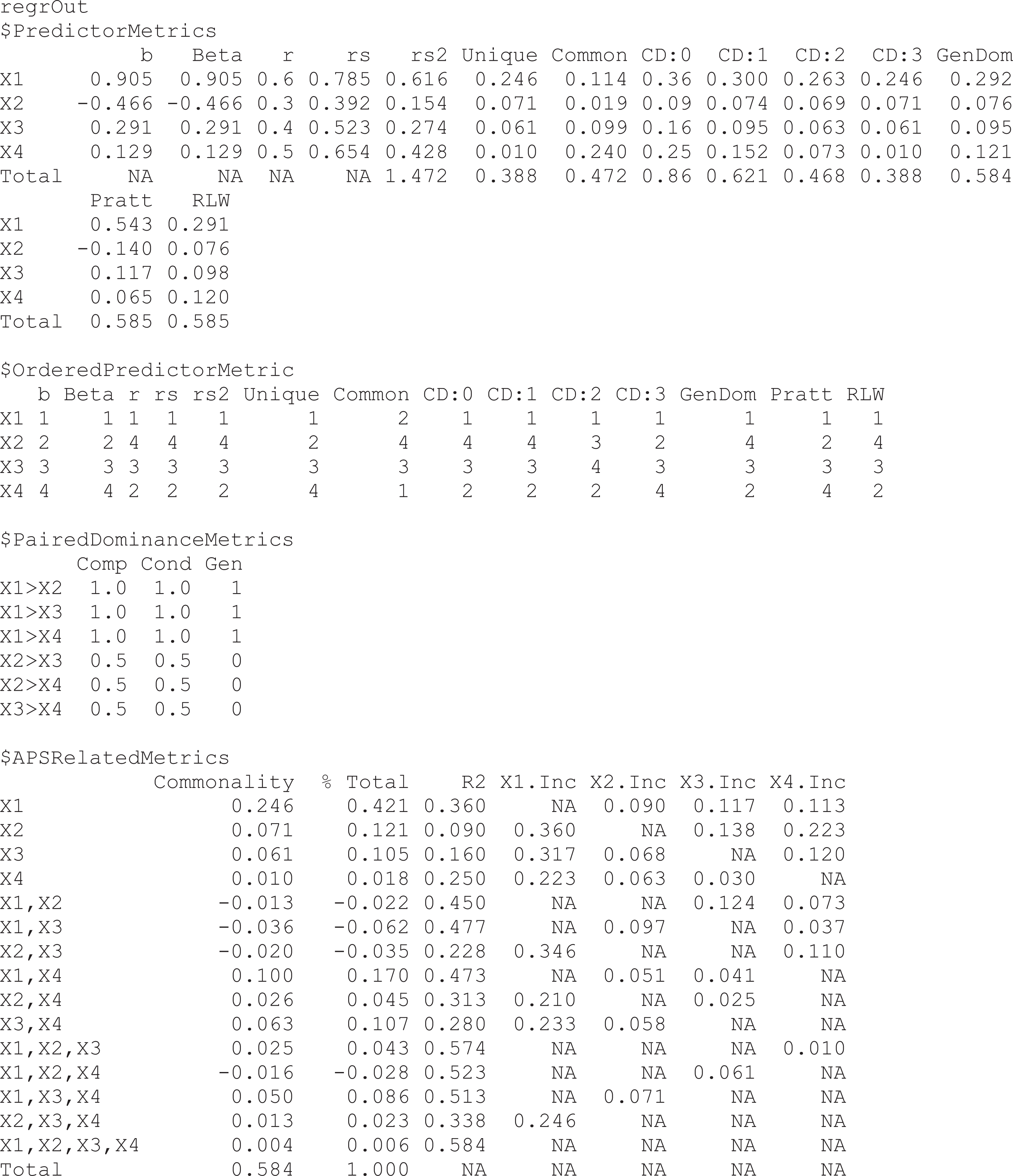
Output from calc.yhat for illustrative example.

The bs and betas values and ranks are identical, as expected with a data set whose variables have been standardized to have Ms of 0 and SDs of 1. The uniqueness coefficients and the conditional dominance weights for k = 3 (i.e., CD:3) are always identical, because both identify the amount of predictive variance that is unique to a predictor. Also note that the order of the b and betas agrees with the order of the uniqueness coefficients, and the order of the validity (r), structure (rs), squared structure coefficients (r_s ²), and squared validity (CD:0) are identical. The former agreement is in line with Nunnally and Bernstein (1994), who noted that unique coefficients and b weights generate the same p values. The latter agreement is aligned with Courville and Thompson (2001), who point out that structure coefficients are rescaled validity coefficients. The similarity between the general dominance (GenDom) and relative weights (RLW) is in keeping with research that indicates that these coefficients typically yield almost identical values, despite different definitions and computational strategies (see Johnson, 2000; LeBreton et al., 2004).

The Pratt weights diverge from the general dominance and relative weights, even though they also sum to equal the R². This divergence likely stems from a disagreement in the signs of X ₂’s beta and validity coefficient, which is suggestive of a suppression effect (cf. Thompson, 2006). However, the conditional dominance weights do not highlight X ₂ as a suppressor because the conditional dominance weights for X ₂ (i.e., CD:0, CD:1, CD:2, CD:3) do not increase as subset models become more complex (cf. Azen & Budescu, 2003; Beckstead, 2012).

The D_ij values in the PairedDominanceMetrics set reflect some of the information revealed by the PredictorMetrics set. The D_ij values for general dominance (Gen) are reflective of the order of the general dominance weights (i.e., X ₁ > X ₄ > X ₃ > X ₂). The D_ij values for conditional dominance (Cond) indicate that across regression models of different subset sizes (i.e., k), X ₁ conditionally dominates the other predictors (i.e., X ₁ > X ₂, X ₃, X ₄) and contributes more incremental variance on average to models of different subsets than the other predictors. The D_ij values for complete dominance reflect information not previously presented and indicate that X ₁ completely dominates all other predictors (i.e., X ₁ > X ₂, X ₃, X ₄).

In reviewing the APSRelatedMetrics set, note that the uniqueness coefficients and squared validity coefficients are redundant with what is reported in the PredictorMetrics set. This is done for ease of interpretation in either set. The commonality coefficients (Commonality) in the APSRelatedMetrics set confirm suppression in the regression model. In particular, they identify suppression involving the following subsets of independent variables: X ₁ and X ₂, X ₁ and X ₃, X ₂ and X ₃, and X ₁, X ₂, and X ₄. The APSRelatedMetrics set contains the results of the APS regression and shows, for example, that there is little difference in the multiple R² produced from the regression model with variables X ₁, X ₂, and X ₃ (R² = .523) and the regression model with variables X ₁, X ₃, and X ₄ (R² = .513). Finally, the APSRelatedMetrics identify the amount of variance each predictor adds to each subset model, which can be used to understand the determination of complete dominance. One sees, for example, that X ₄ does not completely dominate X ₂ because X ₂ (i.e., .097) adds less variance to the regression model with X ₁ and X ₃ than does X ₄ (i.e., .037).

booteval.yhat and plotCI.yhat

Figure 2 presents the bootstrapped CIs around select coefficients from the PredictorMetrics set. Note that with few exceptions (e.g., betas for X ₁ and X ₂, product measures for X ₁ and X ₂, relative weights for X ₁ and X ₂), it is difficult to determine visually whether or not a pair of predictor metrics differs by a statistically significant amount. However, differences between predictor coefficients can easily be seen in Figure 3. The CIs that are indicated with an asterisk (*) identify differences between pairs of predictor coefficients that are statistically significantly different from zero. One sees that across metrics, X ₁ tends to produce coefficients that are statistically significantly greater than the remaining predictors. The exception to this rule involves X ₄ where its structure coefficient (rs), squared validity coefficient (CD:0), conditional dominance weight for k = 1 (CD:1) are statistically equivalent to X ₁’s. Also note that with the exception of X ₃ and X ₄, all betas are statistically significant from one another and that the structure coefficient, squared validity coefficient, and product measure (Pratt) for X ₂ are statistically significantly different from X ₄’s.

Figure 2.

Output from plot.yhat for select predictor metrics from illustrative example.

Figure 3.

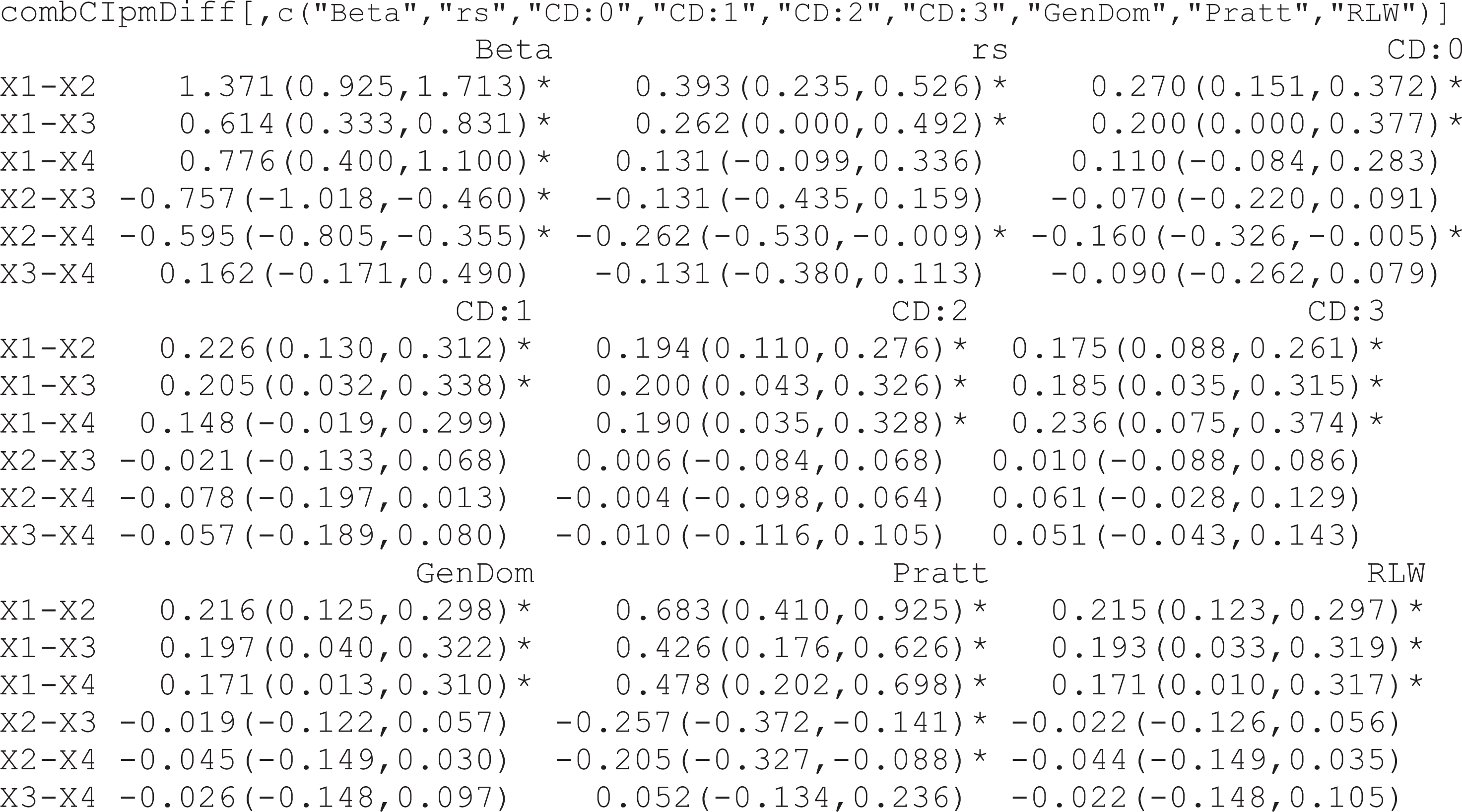
Select predictor metric differences from booteval.yhat for illustrative example.

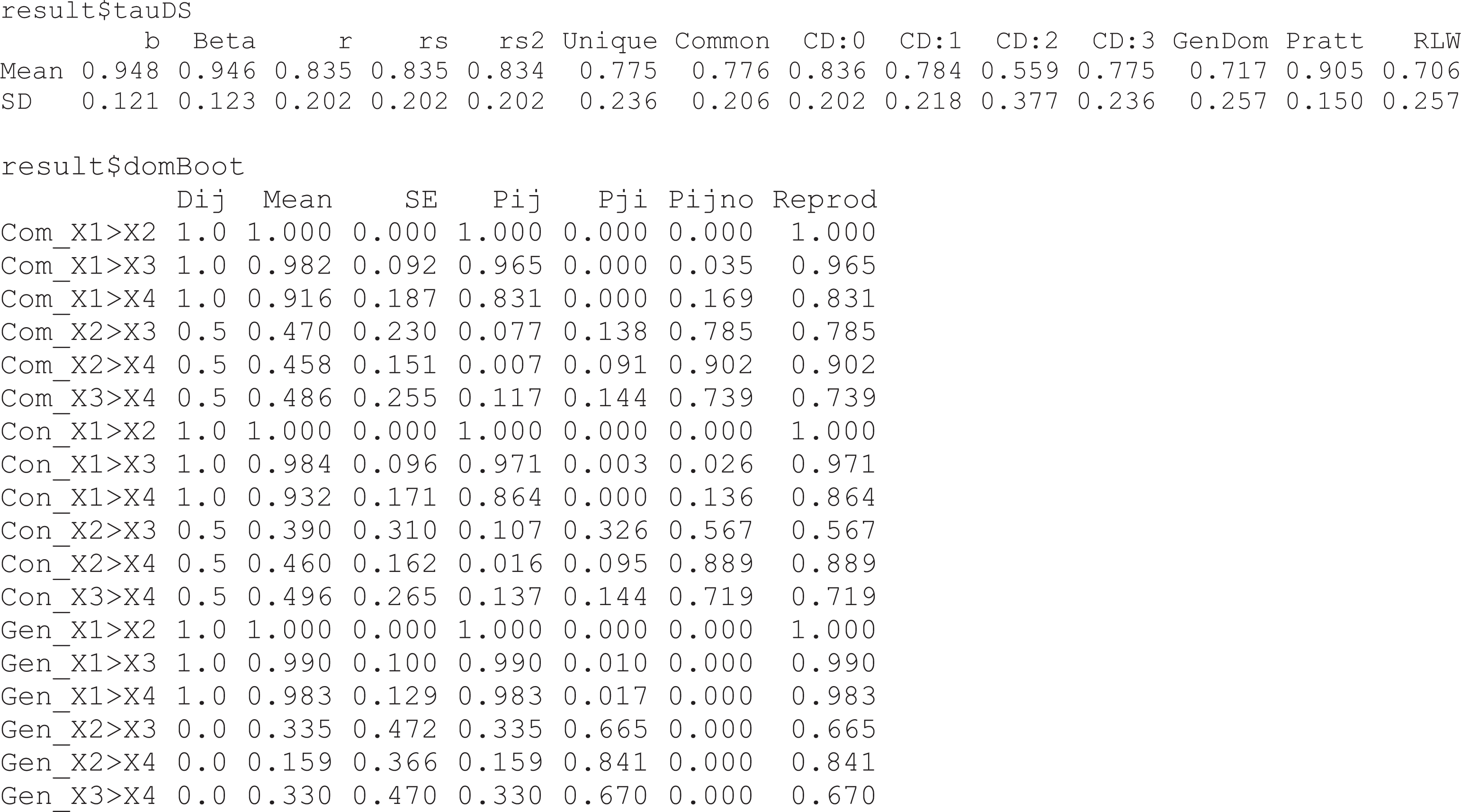
Figure 4 presents the descriptive statistics of the bootstrapped Kendall’s tau correlation between the sample predictor metrics and the bootstrap statistics of like metrics. Across metrics, the order of b and betas (Ms = .948, .946) was most reproducible across bootstrapped samples. Note that the variance of the correlations across bootstraps is lower as the mean of the correlations is higher (in fact, the correlation between the mean and variance across metrics was –.98). Figure 4 also presents the sample D_ij values along with their Ms, SEs, and probabilities and reproducibility over the 1,000 bootstrap samples. It is interesting to note that X ₁ completely dominated X ₂ in each of the bootstrapped samples. Given the hierarchical nature of dominance analyses, X ₁ also conditionally and generally dominated X ₂ in each of the bootstrapped samples.

Figure 4.

Descriptive statistics output from booteval.yhat for illustrative example.

Figure 5 presents the bootstrapped CIs around the coefficients in the APSRelatedMetrics set. Note that the CIs around the uniqueness coefficients and the squared validity coefficients found in Figure 3 are also presented in Figure 5, for ease of interpretation. With only a few nonoverlapping CIs, it is difficult to visually identify statistically significant differences among pairs of coefficients. However, statistically significant differences between APS-related coefficients can readily be seen in Figures 6 and 7, indicated by an asterisk next to the CIs for pairs of APS-related coefficients that are statistically significantly different from zero. One sees, for example, that a majority of the joint variance components involving two predictors are statistically significant different from one another (e.g., X ₁, X ₃ vs. X ₁, X ₄; X ₂, X ₃ vs. X ₃, X ₄). One also sees out of the 15 comparisons involving regression models with k = 2, 7 contained statistically significant differences in multiple R²s; for the 6 comparisons involving regression models with k = 3, 3 contained statistically significant differences in multiple R²s. One can also see that X ₁ did not completely dominate X ₄ across bootstrapped samples because of statistically nonsignificant differences in incremental variance in the cases where k = 0 and where k = 1.

Figure 5.

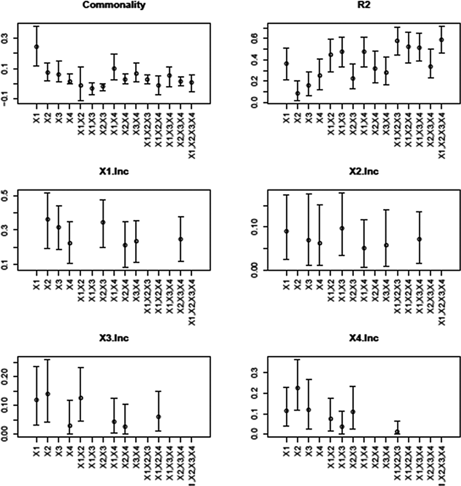
Output from plot.yhat for all-possible-subsets (APS)–related metrics from illustrative example.

Figure 6.

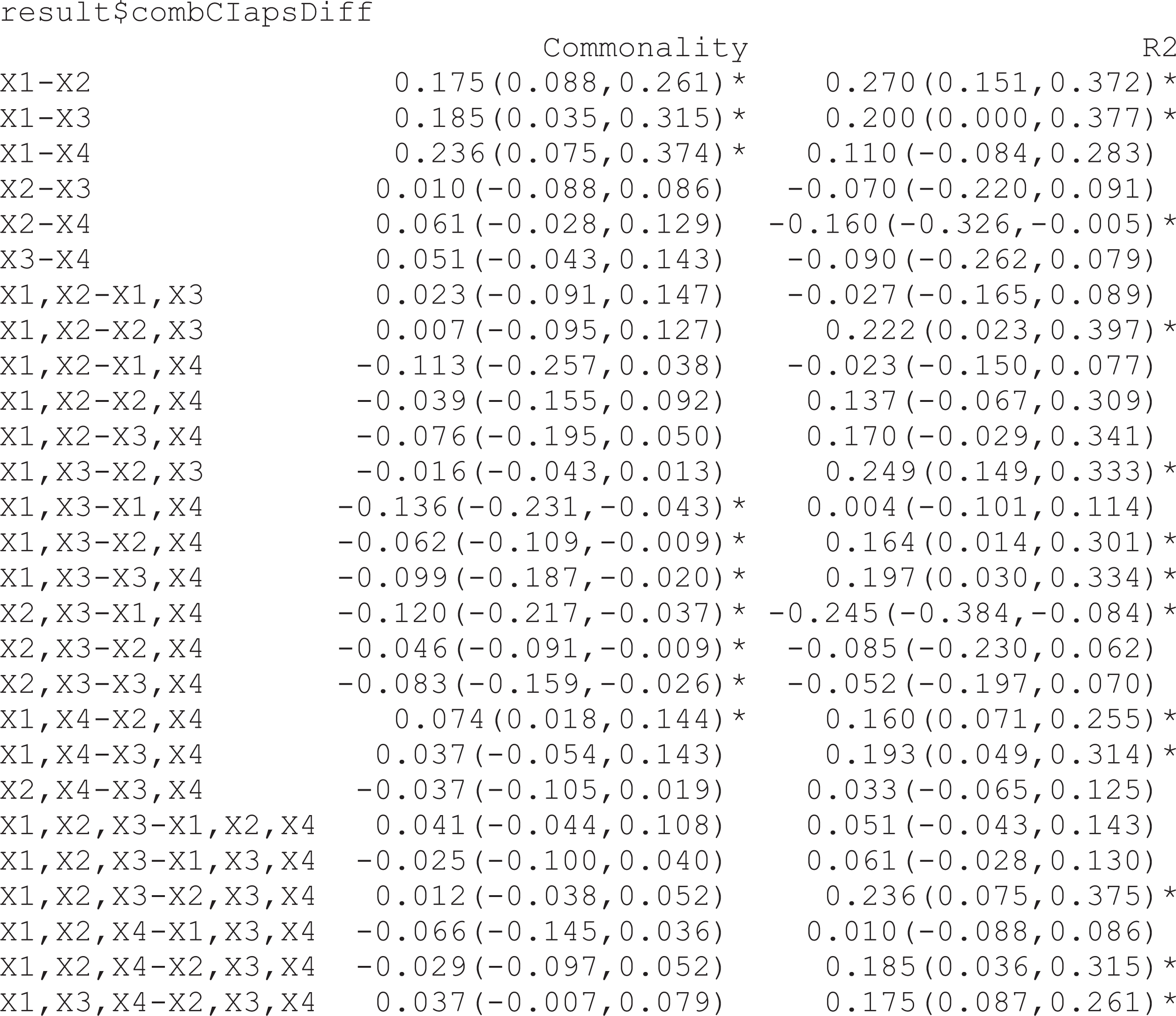
Commonality coefficient and R² differences from booteval.yhat for illustrative example.

Figure 7.

Incremental predictor variance differences from booteval.yhat for illustrative example.

Illustrative Example 2

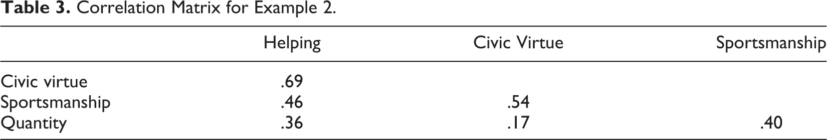
We also conducted a secondary data analysis on the correlation matrix reported in Podsakoff, Ahearne, and MacKenzie (1997) to provide an illustrative example of how one might write up the results from the software presented in this article to be suitable for publication. We examined the model that regressed work crew (n = 40) quantity on “crew members’ assessments of their crews’ helping behavior, civic virtue, and sportsmanship…aggregated at the work group level” (p. 265). We selected the model as it has been previously identified in the literature (e.g., Courville & Thompson, 2001; Nimon & Reio, 2011) as a model that benefitted from examining multiple metrics. Although prior literature has examined the regression model using bs, betas, r_s s, and commonality coefficients, it does not appear that the model has been examined using other metrics presented in this article, including dominance analysis or relative weights. To analyze their model, we modified the example code previously presented to accommodate their correlation matrix, which we present in Table 3.

Table 3.

Correlation Matrix for Example 2.

	Helping	Civic Virtue	Sportsmanship
Civic virtue	.69
Sportsmanship	.46	.54
Quantity	.36	.17	.40

Results for Illustrative Example 2

The model that regressed aggregated civic virtue, sportsmanship, and helping behavior on work crew quality was statistically and practically significant, F(3, 36) = 3.886, p = .017, R² = .247. The aggregated organizational citizenship behaviors explained ∼25% of the variance in work crew quality. Tables 4 and 5, respectively, present the predictor and APS-related metrics, including 95% accelerated bootstrap confidence intervals that were produced over 1,000 iterations.

Table 4.

Predictor Metrics for Example 2.

Metric	Civic Virtue	Sportsmanship	Helping Behavior
Beta	–.314 (–.785, .087)	.386 (–.011,. 713)	.399 (.023, .826)
r	.170 (–.092, .480)	.400 (.074, .639)	.360 (.035, .605)
r_s	.344 (–.280, .803)	.809 (.247, .982)	.728 (.172, .982)
r_s ²	.118 (.000, .605)	.654 (.061, .964)	.530 (.045, .969)
Unique	.045 (.000, .235)	.103 (.001, .353)	.082 (.003, .331)
Common	–.016 (–.225, .170)	.057 (–.064, .249)	.048 (–.079, .280)
CD:0	.029 (.000, .226)	.160 (.006, .408)	.130 (.003, .367)
CD:1	.007 (.000, .034)	.102 (.004, .332)	.076 (.003, .264)
CD:2	.045 (.000, .235)	.103 (.001, .353)	.082 (.003, .331)
GenDom	.027 (.002, .059)	.122 (.006, .336)	.096 (.006, .287)
Pratt	–.053 (–.242, .003)	.154 (–.001, .419)	.144 (.003, .447)
RLW	.024 (.002, .051)	.124 (.007, .332)	.097 (.006, .278)

Note: Unique = uniqueness coefficient; common = R² – uniqueness; CD = conditional dominance weights; GenDom = general dominance weights; Pratt = Pratt measure; RLW = relative weights.

Table 5.

All-Possible-Subset–Related Metrics for Example 2.

Subset	Commonality	R ²	Civ.Inc	Sprt.Inc	Help.Inc
Civ	.045 (.000, .235)	.029 (.000, .226)	NA	.134 (.002, .389)	.112 (.003,. 350)
Sprt	.103 (.001, .353)	.160 (.006, .408)	.003 (0, .030)	NA	.039 (.000, .232)
Help	.082 (.003, .331)	.130 (.003, .367)	.012 (0, .112)	.070 (.000, .301)	NA
CivSprt	–.034 (–.166, .005)	.163 (.009, .388)	NA	NA	.082 (.003, .331)
CivHelp	–.042 (–.208, .016)	.141 (.007, .361)	NA	.103 (.001, .353)	NA
SprtHelp	.031 (–.011, .173)	.199 (.013, .424)	.045 (0, .235)	NA	NA
CivSprtHelp	.060 (–.007, .225)	.245 (.024, .435)	NA	NA	NA

Note: Civ = civic virtue; Sprt = sportsmanship; Help = helping behavior.

With the exception of betas that identify helping behavior as the most important predictor, followed by sportsmanship and civic virtue, the remaining predictor metrics identify sportsmanship as the most important predictor and helping behavior as the second most important predictor. This means that although sportsmanship (a) shares the most variance with the work crew quality and predicted work crew quality, (b) contributes the most unique and common variance to work crew quality, (c) adds the most incremental variance, on average, to models of different subsizes, and (d) accounts for the largest partition of R² as computed with general dominance weights, Pratt measures, and relative weights, helping behavior is given the greatest credit in the regression equation. The predictor metrics also identify civic virtue as a suppressor variable. In addition to it contributing more unique variance to the regression effect than it has in common with the work crew quality and yielding a negative Pratt’s measure (as a result of inconsistent signs between its beta and validity coefficient), the conditional dominance weights for civic virtue do not decrease monotonically with more complex models (cf. Azen & Budescu, 2003).

The APS-related metrics show that civic virtue contributes the most incremental variance when added to a regression model that contains sportsmanship and helping behavior and that its addition suppresses irrelevant variance in sportsmanship and helping behavior, making them better predictors than if civic virtue was not included. This means that if sportsmanship and helping behavior are to have maximum impact in predicting work crew quality, the measures should be refined to eliminate irrelevant variance related to civic virtue. Analysis of the bivariate correlations and the incremental validity coefficients reported in Table 4 indicates that sportsmanship completely dominates helping behavior, which completely dominates civic virtue. This means that across all possible subset models, (a) sportsmanship adds more incremental variance than helping behavior and civic virtue and (b) helping behavior adds more incremental variance than civic virtue.

It is important to note that many of the study’s findings may not be replicable, given its small sample size. Across bootstrapped samples, the predictor order based on betas was most consistent with the sample data. As presented in Table 6, the average Kendall’s tau, correlating beta weight-based predictor order from bootstraps to sample data, was .641 (SD = .367). Predictor order based on unique variance was least replicable (M = .353, SD = .540). Bootstrap analysis of differences between predictor metrics found only a few statistically significant differences (see Table 7). Bootstrap analyses of differences between appropriate APS metrics found no statistically significant differences. For each order of predictor combinations, there were no statistically significant differences among the multiple R² or commonality coefficient produced, nor were there statistically significant differences among the predictors’ incremental validity coefficients.

Table 6.

Descriptive Statistics for Kendall’s Tau Across Bootstrap Iterations.

Metric	M	SD
Beta	.641	.367
r	.668	.415
r_s	.667	.415
r_s ²	.645	.435
Unique	.353	.540
Common	.554	.521
CD:0	.646	.434
CD:1	.531	.492
CD:2	.353	.540
GenDom	.530	.490
Pratt	.634	.402
RLW	.566	.480

Note: Unique = uniqueness coefficient; common = R² – uniqueness; CD = conditional dominance weights; GenDom = general dominance weights; Pratt = Pratt measure; RLW = relative weights.

Table 7.

Differences in Predictor Metrics for Example 2.

Metric	Civ-Sprt	Civ-Help	Sprt-Help
Beta	–.700 (–1.367, –.065)*	–.713 (–1.543, –.042)*	–.013 (–.738, .489)
r	–.230 (–.523, .039)	–.190 (–.457, .012)	.040 (–.313, .354)
r_s	–.465 (–.977, .050)	–.384 (–.846, –.013)*	.081 (–.601, .710)
r_s ²	–.536 (–.906, –.026)*	–.412 (–.806, –.024)*	.124 (–.715, .813)
Unique	–.058 (–.308, .093)	–.037 (–.246, .056)	.021 (–.275, .298)
Common	–.073 (–.301, .005)	–.064 (–.230, .003)	.009 (–.042, .166)
CD:0	–.131 (–.388, .009)	–.101 (–.284, .003)	.030 (–.213, .288)
CD:1	–.095 (–.340, .030)	–.069 (–.250, .017)	.026 (–.232, .293)
CD:2	–.058 (–.308, .093)	–.037 (–.246, .056)	.021 (–.275, .298)
GenDom	–.095 (–.340, .030)	–.069 (–.249, .016)	.026 (–.231, .294)
Pratt	–.207 (–.557, –.004)*	–.197 (–.626, .001)	.010 (–.415, .330)
RLW	–.100 (–.340, .021)	–.073 (–.245, .014)	.027 (–.219, .288)

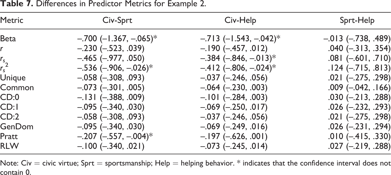
Note: Civ = civic virtue; Sprt = sportsmanship; Help = helping behavior. * indicates that the confidence interval does not contain 0.

Discussion

Although the interpretation of linear regression weights is straightforward when the goal is prediction, it has long been known that when the goal of a regression analysis is instead to make some conclusions about the relative importance of the predictors in the model, the intercorrelations between predictors (multicollinearity) undermine the use of regression weights for this purpose. Alternative metrics are required—and perhaps more than one set of metrics is interesting to consider because each is operationalized differently and carries different assumptions. Specific to the current article, we review regression weights, zero-order validity coefficients, structure coefficients, Pratt measures, relative importance weights, all-possible-subsets regression, commonality coefficients, and dominance weights.

Perhaps more important than this review of a wide range of metrics relevant to linear regression, our article offers a freely available software package in R code that (a) computes all of these indices at once, (b) computes associated bootstrapped confidence intervals, (c) compares pairs of predictors against one another in terms of their bootstrapped metric, and (d) performs these contributions for any number of predictors so long as the correlation matrix is positive definite (invertible). Other software is limited in all four respects.

We hope researchers will use this software to change their fundamental approach to conducting and interpreting linear regression analysis as applied to their data. Given the variety of weights available, it can be informative to consider an array of weights and to report the most appropriate importance weights, or to examine how they converge and diverge, rather than merely focus on the weights that are the most popular or typically available. The program we offer obviously requires the expertise of the researcher or practitioner to determine which set or sets of importance weights are most appropriate to report. Fortunately, Nathans et al. (2012) provided an accessible treatment of the metrics reported by the software presented along with strengths, limitations, and recommendations for practice. This along with other works that also address predictor importance in detail (e.g., Budescu & Azen, 2004; LeBreton et al., 2004) and the examples in the current article should provide researchers a general template for their own work in interpreting and reporting MLR models.

Although the regression indices we have reviewed can be informative, and the software can be a useful tool to make use of these indices, there are several avenues for future research that extend beyond the current purview. First, it is possible that the study of some psychological phenomena requires multiple criteria as well as multiple predictors, leading to a complex canonical prediction problem (e.g., Azen & Budescu, 2006; LeBreton & Tonidandel, 2008; Nimon, Henson, & Gates, 2010). Second, another frequent concern is the reliability or stability of importance-weight estimates across independent samples to which a regression model is supposed to generalize (e.g., Azen & Budescu, 2003; Johnson, 2004). We implemented bootstrapping to compute standard errors of the coefficients for all metrics and to address directly the problem of stability in a random sample; however, there is no guarantee that similar results would be obtained in a nonrandom sample, in particular a sample that is supposed to exhibit the same pattern of relationships and variable importance but that is a substantively different sample from the first one (e.g., an Army sample vs. an Air Force sample). Thus, research could examine replication and generalizability of these MLR metrics across samples of varying degrees of generalizability.

Third, we provide information on the submodels from all-possible-subsets regression for further investigation, and future research could quickly apply statistical and graphical exploratory tools to represent and test patterns within APS that go beyond the submodel summaries provided by general and conditional dominance analysis. Fourth, future research could consider MLR models that remain linear in their parameter estimates but include interaction terms and/or nonlinear terms, which would likely raise additional considerations (Dalal & Zickar, 2012). Perhaps many of these metrics could be extended to the hierarchical regression analysis framework; this might be something like APS yet would impose constraints or a structure on the sets of models to be tested. Fifth and finally, although we have covered a wide range of metrics, we also realize that other metrics could eventually be incorporated into the yhat package (e.g., the Lasso method and its variants, Tibshirani, 1996; Bayesian variable selection, Mitchell & Beauchamp, 1988; Bayesian model averaging, Raftery, Madigan, & Hoeting, 1997).

Although all of these suggestions might prove worthy of consideration in future research, it was beyond the scope of this article to address them in detail. Again, our main focus is in providing a comprehensive and freely available program useful for bringing together and generating different types of predictor importance metrics in multiple regression analysis and to provide empirical examples that accompany the program, both of which we hope will allow researchers to think about and conduct regression analysis in a fundamentally different manner. Previously, such metrics were examined in isolation, often without much consideration of the other metrics available. Thus, regular use of the program in the future will hopefully provide researchers with new insights and guidance for the use of regression metrics that nobody—including ourselves—has yet offered.

Consider the work of Seibold and McPhee (1979) who examined the impact that cognition and social affect had in minority women’s intent to get a cancer screening test. Had the researchers only considered betas, they would have missed identifying cognition as a suppressor variable and the need to purify cognitive relevance from screening messages aimed at addressing social affect in order to have the maximum impact on intentions. To generalize from this example, we believe and envision that the software described can become an essential tool in substantive research, to understand the predictive relationships and interrelationships among variables in regression models more closely and from different perspectives, as well as in simulation research, to understand and appreciate statistical conditions that cause convergence and divergence among different regression metrics (extending the foundational work of LeBreton et al., 2004). Without conducting such detailed analyses, researchers may miss detecting and interpreting valuable relationships in their data.

Footnotes

Appendix

Declaration of Conflicting Interests

The author(s) declared no potential conflicts of interest with respect to the research, authorship, and/or publication of this article.

Funding

The author(s) received no financial support for the research, authorship, and/or publication of this article.

References

Algina

Keselman

H. J.

Penfield

R. D.

(2010). Confidence intervals for squared semipartial correlation coefficients: The effect of nonnormality. Educational and Psychological Measurement, 70, 926–940.

Azen

Budescu

D. V.

(2003). The dominance analysis approach for comparing predictors in multiple regression. Psychological Methods, 8, 129–148.

Azen

Budescu

D. V.

(2006). Comparing predictors in multivariate regression models: An extension of dominance analysis. Journal of Educational and Behavioral Statistics, 31, 157–180.

Beckstead

J. W.

(2012). Isolation and examining source of suppression and multicollinearity in multiple linear regression. Multivariate Behavioral Research, 47, 224–246.

Braun

M. T.

Oswald

F. L.

(2011). Exploratory regression analysis: A tool for selecting models and determining predictor importance. Behavioral Research Methods, 43, 331–339.

Budescu

D. V.

(1993). Dominance analysis: A new approach to the problem of relative importance of predictors in multiple regression. Psychological Bulletin, 114, 542–551.

Budescu

D. V.

Azen

(2004). Beyond global measures of relative importance: Some insights from dominance analysis. Organizational Research Methods, 7, 341–350.

Canty

Ripley

(2011). boot: Bootstrap R (S-Plus) functions (R package version 1.3-2) [Computer software].

Chevan

Sutherland

(1991). Hierarchical partitioning. The American Statistician, 45, 90–96.

10.

Courville

Thompson

(2001). Use of structure coefficients in published multiple regression articles: β is not enough. Educational and Psychological Measurement, 61, 229–248.

11.

Culpepper

S. A.

Aguinis

(2011). R is for revolution: A cutting-edge, free, open source statistical package. Organizational Research Methods, 14, 735–740.

12.

Cumming

Finch

(2001). A primer on the understanding, use, and calculation of confidence intervals that are based on central and noncentral distributions. Educational and Psychological Measurement, 61, 532–574.

13.

Cumming

Finch

(2005). Inference by eye: Confidence intervals and how to read pictures of data. American Psychologist, 60, 170–180.

14.

Dalal

D. K.

Zickar

M. J.

(2012). Some common myths about centering predictors in moderated multiple regression and polynomial regression. Organizational Research Methods, 15, 339–362.

15.

Darlington

R. B.

(1968). Multiple regression in psychological research and practice. Psychological Bulletin, 69, 161–182.

16.

Fabbris

(1980). Measures of predictor variable importance in multiple regression: An additional suggestion. Quality & Quantity, 4, 787–792.

17.

Genizi

(1993). Decomposition of R² in multiple regression with correlated regressors. Statistica Sinica, 3, 407–420.

18.

Grömping

(2006). Relative importance for linear regression in R: The package relaimpo. Journal of Statistical Software, 17, 1–27.

19.

Hedges

L. V.

Olkin

(1981). The asymptotic distribution of commonality coefficients. Psychometrika, 46, 331–336.

20.

Johnson

J. W.

(2000). A heuristic method for estimating the relative weight of predictor variables in multiple regression. Multivariate Behavioral Research, 35, 1–19.

21.

Johnson

J. W.

(2004). Factors affecting relative weights: The influence of sampling and measurement error. Organizational Research Methods, 7, 283–299.

22.

Johnson

J. W.

LeBreton

J. M.

(2004). History and use of relative importance indices in organizational research. Organizational Research Methods, 7, 238–257.

23.

Kraha

Turner

Nimon

Zientek

Henson

(2012). The multifaceted concept of predictor importance: Tools to support interpreting multiple regression. Frontiers in Psychology, 3(44), 1–16.

24.

Krasikova

LeBreton

J. M.

Tonidandel

(2011). Estimating the relative importance of variables in multiple regression models. In Hodgkinson

G. P.

Ford

J. K.

(Eds.), International review of industrial and organizational psychology (Vol. 26, pp. 119–141). Indianapolis, IN: Wiley.

25.

LeBreton

J. M.

Ployhart

R. E.

Ladd

R. T.

(2004). A Monte Carlo comparison of relative importance methodologies. Organizational Research Methods, 7, 258–282.

26.

LeBreton

J. M.

Tonidandel

(2008). Multivariate relative importance: Relative weight analysis to multivariate criterion spaces. Journal of Applied Psychology, 93, 329–345.

27.

Lindeman

R. H.

Merenda

P. F.

Gold

R. Z.

(1980). Introduction to bivariate and multivariate analysis. Glenview, IL: Scott, Foresman and Company.

28.

Lorenzo-Seva

Ferrando

P. J.

Chico

(2010). Two SPSS programs for interpreting multiple regression results. Behavior Research Methods, 42, 29–35.

29.

Mayeske

G. W.

Cohen

W. M.

Wisler

C. E.

Okada

Beaton

A. E.

Proshek

J. M.

Tabler

K. A.

(1969). A study of our nation’s schools. Washington, DC: U.S. Department of Health, Education, and Welfare, Office of Education.

30.

Mitchell

T. J.

Beauchamp

J. J.

(1988). Bayesian variable selection in linear regression. Journal of the American Statistical Association, 83, 1023–1032.

31.

Mood

A. M.

(1969). Macro-analysis of the American educational system. Operations Research, 17, 770–784.

32.

Mood

A. M.

(1971). Partitioning variance in multiple regression analyses as a tool for developing learning models. American Educational Research Journal, 8, 191–202.

33.

Nathans

L. L.

Oswald

F. L.

Nimon

(2012). Interpreting multiple regression: A guidebook of variable importance. Practical Assessment, Research & Evaluation, 9, 1–19.

34.

Newton

R. G.

Spurrell

D. J.

(1967). A development of multiple regression for the analysis of routine data. Applied Statistics, 16, 51–64.

35.

Nimon

Gavrilova

Roberts

J. K.

(2010). Regression results in human resource development research: Are we reporting enough? In Graham

Dirani

(Eds.), Proceedings of the Human Resource Development 2010 International Conference (pp. 803–812), Knoxville, TN: AHRD.

36.

Nimon

Henson

Gates

(2010). Revisiting interpretation of canonical correlation analysis: A tutorial and software solution for canonical commonality analysis. Multivariate Behavioral Research, 45, 702–724.

37.

Nimon

Reio

(2011). Regression commonality analysis: A technique for quantitative theory building. Human Resource Development Review, 10, 329–340.

38.

Nimon

Roberts

J. K.

(2012). yhat: Interpreting regression effects (R package version 1.0-5) [Computer software]. Retrieved from http://CRAN.R-project.org/package=yhat

39.

Nunnally

J. C.

Bernstein

I. H.

(1994). Psychometric theory (3rd ed.). New York, NY: McGraw-Hill.

40.

Onwuegbuzie

A. J.

Daniel

L. G.

(2003, February 19). Typology of analytical and interpretational errors in quantitative and qualitative educational research. Current Issues in Education, 6(2). Retrieved from http://cie.asu.edu/volume6/number2/

41.

Podsakoff

P. M.

Ahearne

MacKenzie

S. B.

(1997). Organizational citizenship behavior and the quantity and quality of work group performance. Journal of Applied Psychology, 82, 262–270.

42.

Pratt

J. W.

(1987). Dividing the indivisible: Using simple symmetry to partition variance explained. In Pukkila

Puntanen

(Eds.), Proceedings of the second international Tampere conference in statistics (pp. 245–260). Tampere, Finland: University of Tampere.

43.

R Development Core Team. (2013). R: A language and environment for statistical computing [Computer software]. Vienna, Austria: R Foundation for Statistical Computing. Retrieved from http://www.R-project.org/

44.

Raftery

A. E.

Madigan

Hoeting

J. A.

(1997). Bayesian model averaging for linear regression models. Journal of the American Statistical Association, 92, 179–191.

45.

Rowell

R. K.

(1996). Partitioning predicted variance into constituent parts: How to conduct regression commonality analysis. In Thompson

(Ed.), Advances in social science methodology (Vol. 4, pp. 33–43). Greenwich, CT: JAI Press.

46.

Schoen

J. L.

DeSimone

J. A.

James

L. R.

(2011). Exploring joint variance between independent variables and a criterion: Meaning, effect, and sizes. Organizational Research Methods, 14, 674–695.

47.

Seibold

D. R.

McPhee

R. D.

(1979). Commonality analysis: A method for decomposing explained variance in multiple regression analysis. Human Communication Research, 5, 355–363.

48.

Thomas

D. R.

Hughes

Zumbo

B. D.

(1998). On variable importance in linear regression. Social Indicators Research, 45, 253–275.

49.

Thompson

(2006). Foundations of behavioral statistics: An insight-based approach. New York, NY: Guilford Press.

50.

Tibshirani

(1996). Regression shrinkage and selection via the lasso. Journal of the Royal Statistical Society B, 51, 267–288.

51.

Tonidandel

LeBreton

J. M.

(2011). Relative importance analysis—A useful supplement to regression analyses. Journal of Business and Psychology, 26, 1–9.

52.

Tonidandel

LeBreton

J. M.

Johnson

J. W.

(2009). Statistical significance tests for relative weights. Psychological Methods, 14, 387–399.

53.

Zientek

L. R.

Capraro

M. M.

Capraro

R. M.

(2008). Reporting practices in quantitative teacher education research: One look at the evidence cited in the AERA panel report. Educational Researcher, 34, 208–216.

54.

Zientek

L. R.

Thompson

(2006). Commonality analysis: Partitioning variance to facilitate better understanding of data. Journal of Early Intervention, 28, 299–307.

55.

Zientek

L. R.

Yetkiner

Z. E.

Thompson

(2010). Characterizing the mathematics anxiety literature using confidence intervals as a literature review mechanism. The Journal of Educational Research, 103, 424–438.