The Effects of Chance Correlations on Partial Least Squares Path Modeling

Abstract

Partial least squares path modeling (PLS) has been increasing in popularity as a form of or an alternative to structural equation modeling (SEM) and has currently considerable momentum in some management disciplines. Despite recent criticism toward the method, most existing studies analyzing the performance of PLS have reached positive conclusions. This article shows that most of the evidence for the usefulness of the method has been a misinterpretation. The analysis presented shows that PLS amplifies the effects of chance correlations in a unique way and this effect explains prior simulations results better than the previous interpretations. It is unlikely that a researcher would willingly amplify error, and therefore the results show that the usefulness of the PLS method is a fallacy. There are much better ways to compensate for the attenuation effect caused by using latent variable scores to estimate SEM models than creating a bias into the opposite direction.

Keywords

partial least squares structural equation modeling chance correlations Monte Carlo simulation

Partial least squares path modeling (PLS) has recently gained popularity in several disciplines as an alternative approach to structural equation modeling (SEM) or as an alternative to SEM (Hair, Sarstedt, Ringle, & Mena, 2012; Ringle, Sarstedt, & Straub, 2012; Rönkkö & Evermann, 2013). The route through which PLS emerged into the mainstream is rather unorthodox. The PLS method was initially developed by the econometrician Herman Wold (Dijkstra, 2010; Wold, 1982), but the method never gained much attention from other econometricians or other researchers specializing in statistical analysis, and consequently the PLS method is currently almost nonexistent in the mainstream research methods journals (Rönkkö & Evermann, 2013). Instead the method reemerged through the marketing and information systems disciplines (Hair, Ringle, & Sarstedt, 2012), where the popularization of the method can be attributed to a number of introductory articles that present PLS as a SEM method that has less stringent assumptions about the data and avoids many of the perceived difficulties of SEM.

A review of the past 10 years (2003-2012) of papers in all the journals on the Financial Times 45 journal list (“45 Journals Used in FT Research Rank,” 2012) shows that the PLS method is being adopted increasingly but unevenly by many fields where the method has traditionally not been used. Searching the full text content of these journals with term structural equation, confirmatory factor, RMSEA, partial least, and PLS and manually screening the results for papers that used either latent variable SEM or PLS as an analysis method resulted a list of 1,838 studies, of which 247 used PLS. Among those journals that published studies using these methods, the PLS papers were very unevenly distributed. On one extreme, in the Journal of Applied Psychology only 2 papers out of 300 used PLS. This is contrasted against MIS Quarterly and Information Systems Research where 115 of a total of 178 studies used PLS, accounting for almost half of all PLS-based papers on the list of 45 journals. Excluding these 2 information systems journals, 93 of the remaining 128 PLS studies were published during the past 5 years (2008-2012) presenting an almost threefold increase compared to the first 5-year period (2003-2007).

Figure 1 shows the popularity of PLS compared to latent variable SEM in the 15 journals, in which the method was used the most, split into two 5-five year periods. The two information systems journals stand out in the figure being the only two journals where PLS was more popular than latent variable SEM for both time periods. In addition to the large number of empirical applications in MIS Quarterly, there were 13 papers either discussing or analyzing the PLS method, more than in all the other journals combined. Only one of the methodological studies was critical of PLS (Goodhue, Lewis, & Thompson, 2012b), and even this study included a mildly positive assessment of PLS in the conclusions. The enthusiasm on PLS in the information systems community can be explained by a potential bias toward papers that reinforce the status quo in the top information systems journals not unlike the positive bias toward formative measurement observed by Hardin and Marcoulides (2011). On the one hand, papers that advance or reinforce the current methodological practices seem to be accepted, sometimes even without any evidence of the usefulness of the proposed methodological approach (e.g., Liang, Saraf, Hu, & Xue, 2007). On the other hand, some researchers feel that the journals actively discourage papers critically examining the current methodological practices (Goodhue et al., 2012a). There are also a few examples of papers challenging the current methodological stance being rejected by MIS Quarterly and later appearing in research methods journals (Hardin & Marcoulides, 2011; A. Hardin, personal communication, May 1, 2013; Treiblmaier, Bentler, & Mair, 2011; H. Treiblmaier, personal communication, December 5, 2011). The problem of possible positive bias toward PLS in the information systems journals is not limited to the information systems discipline because researchers in other disciplines are drawing on these papers for information about the PLS methods and recent papers are actively encouraging them to do so (Gefen, Rigdon, & Straub, 2011).

Figure 1.

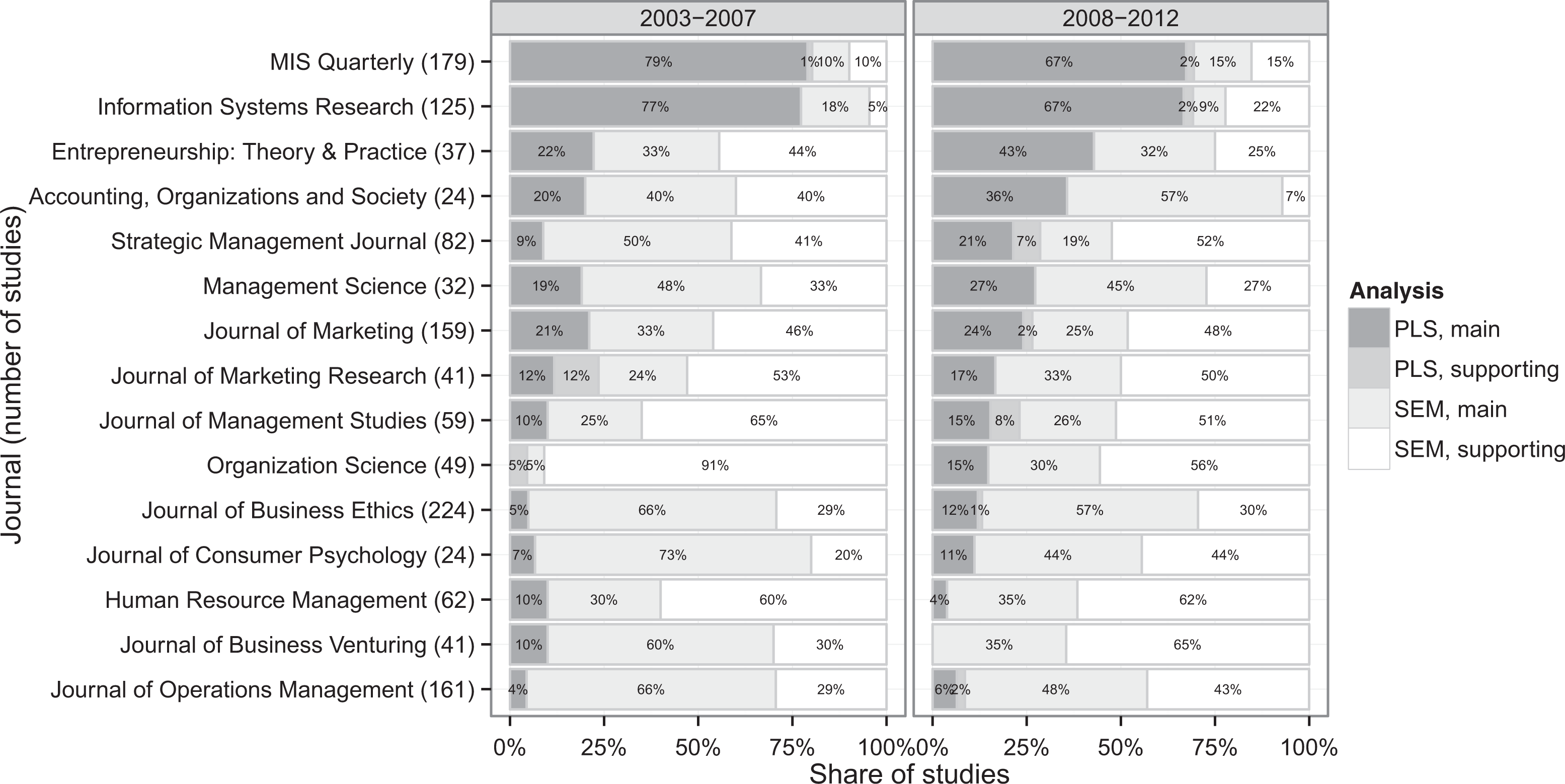
Use of partial least squares (PLS) in high-quality business journals in 2003-2012.

The adoption of PLS in the management disciplines seems to follow a pattern where it is first introduced to a discourse from another discipline by a paper or two that use the method, after which further studies are legitimized by citing these earlier papers. A reviewer who then wants to challenge the legitimacy of PLS may find herself in a difficult position, as the authors now have the prior studies as well as introductory level books (Hair, 2010, Chapter 15; Kline, 2010, pp. 287-288; Rigdon, 2013; Savalei & Bentler, 2007) and multiple introductory articles (e.g., Gefen et al., 2011; Hair, Ringle, et al., 2012; Peng & Lai, 2012) that can be cited to support their methodological choice. While there are some methodological papers that challenge the use of PLS (Goodhue et al., 2012b; Rönkkö & Evermann, 2013), there are many more that reach the opposite conclusions (e.g., Cassel, Hackl, & Westlund, 2000; Chin & Newsted, 1999; Reinartz, Haenlein, & Henseler, 2009), thus making any evidence-based arguments for and against PLS rather unevenly matched. The position of a PLS skeptic is not helped by the fact that the results of both the recent papers have already been challenged: In the case of Goodhue et al. (2012b), Marcoulides, Chin, and Saunders (2012) dismiss the study as an inappropriate comparison due to incorrect parameterization. Similarly, some of the main arguments by Rönkkö and Evermann (2013) were quickly challenged by Henseler et al. (2014; see also McIntosh, Edwards, & Antonakis, 2014).

The papers that are critical of PLS are also hampered by their focus on disproving positive beliefs about the method rather than focusing on the disadvantages. For example, in the case of Goodhue et al. (2012b) the authors showed that PLS does not correct for measurement error, but nevertheless concluded the paper by stating that PLS would be an appropriate method for many situations. Another problem with the existing studies is that they largely fail to explain why some other studies have produced the opposite results. Rönkkö and Evermann (2013) touch this issue by showing that in a simulation with a with two latent variable model, PLS capitalizes strongly on chance correlations—correlations that do not exist in the population, but are non-zero in a sample because of sample variability—between error terms and suggest this as an explanation for the earlier, positive results but nevertheless do not pursue the argument further. In sum, while these papers show that PLS may not have the capabilities that many papers argue it has, they do not directly argue that PLS is altogether a flawed method.

This paper takes a different approach by focusing on what the PLS method actually does, which turns out to be is to capitalize on chance correlations in a way that is not documented in the earlier literature and that also explains the earlier, positive results. The purpose of this paper is twofold: First, the paper provides important, new evidence that a researcher skeptical of PLS can use to support her position. Whereas Rönkkö and Evermann (2013) stated that their study casts strong doubts on the effectiveness of PLS, the evidence presented in this paper should remove any such doubts by showing that what the PLS method actually does is to amplify the effect of chance correlations in a unique way, and this is almost certainly not something that a researcher would want to do. Second, there are ongoing efforts to improve or fix PLS by improving its asymptotic properties (Bentler & Huang, 2014; Dijkstra, 2014; Dijkstra & Henseler, 2012; Dijkstra & Schermelleh-Engel, 2013). These studies correctly observe that PLS is not consistent and introduce changes or corrections that would result in a consistent estimator. This study exposes a previously unknown and serious flaw in PLS that would also need to be addressed to make PLS a useful method for estimating SEM models.

Prior Simulation Evidence on the Performance of the PLS Method

PLS is often presented as a component-based estimator for SEM. No explicit definition for component-based estimation is given in the literature, but there seems to be an implicit understanding that such estimation proceeds in two steps: (1) calculating latent variable scores as weighted linear combinations (composites) of the indicator variables and (2) estimating the relationships between the composites using separate regression analyses (Hwang, Malhotra, Kim, Tomiuk, & Hong, 2010; Lu, Kwan, Thomas, & Cedzynski, 2011; Tenenhaus, 2008). Using this definition, the most typical component-based SEM estimator would be regression with summed scales or factor scores. The distinct feature of PLS and the only difference between these more traditional analysis methods is the iterative indicator weighting system (Chin, Marcolin, & Newsted, 2003; Goodhue et al., 2012b), which is explained in more detail later in the paper.

Regardless of the chosen weighting system, a key weakness in forming composite variables of indicators that contain measurement error is that any estimates produced with these composites will generally be inconsistent, although there are special cases where consistency can be achieved (Lu & Thomas, 2008). The fact that PLS is not consistent is readily acknowledged in the PLS literature (e.g., Chin, 1998). Rather, the argument for PLS has been that there are situations where a consistent estimator (typically ML SEM) may not be available or may perform poorly because of small sample size or violation of assumptions, and in these cases PLS, while inconsistent, would be the best available alternative. In theory, there are indeed some cases where an inconsistent estimator with known bias may be preferable to an unbiased estimator if the bias is well understood and the variance of the biased estimator is small compared to the unbiased one (Lehmann & Casella, 1998, p. 84). However, one cannot categorically conclude that when ML SEM fails or performs poorly, PLS should be used instead because it is possible that one of the other alternative component-based estimation approaches (e.g., regression with summed scales or factor scores) would outperform PLS or that the data are just inappropriate for any statistical analysis.

The lack of consistency of PLS suggests that it should not perform well when compared against consistent SEM estimators. Table 1, which lists prior Monte Carlo studies of PLS, shows that this is indeed generally the case. Interestingly many of the papers also show that when compared to regression analysis with summed scales, PLS results are less biased, suggesting that PLS may have an edge over other component-based estimators. In a recent paper Goodhue et al. (2012b) argued that the difference in bias was not statistically significant, but this conclusion was based on inappropriate use of prediction intervals. When the data were reanalyzed with the appropriate tests, the difference was statistically significant (D. L. Goodhue, personal communication, April 10, 2012). In fact, all the studies that compare bias of regression with summed scales and PLS show that the latter is less biased. The analysis presented later in the paper shows why this happens, why this is the wrong thing to look at, and particularly why this cannot be used as evidence that recent criticism toward PLS would be wrong.

Table 1.

Studies Evaluating Partial Least Squares (PLS) With Monte Carlo Methods.

Study	Study Design						Number of Reported Results Where PLS Estimates Are as Follows:
				Experimental			Compared to Summed Scales:		Larger for
	Conclusions About PLS	Tested Model(s)	Parameter Values	Conditions	Estimators	Analyzed Results	Less Biased	Further From 0	Small Samples
Aguirre-Urreta, Marakas, Ellis, and Sun, 2008	SEM outperforms PLS. PLS results were biased downward. The bias decreases with increasing number of indicators and decreasing sample size, and depends on the model.	2 exog. and 2 endog. LVs with 4 paths.	Loadings: .8 Paths: .2, .3, .4, .5	Sample: 40, 80, 120, 160, 200, 260, 320 MVs: 3, 5, 7, 9, 11	PLS (unspecified)	Bias, SEs, power	NA	NA	81/120
Chin and Newsted, 1999	Partial least squares always performed better (was less biased) than the simple summed regression approach, although it did best at lower numbers of indicators.	1 exog. LV and many endog. LVs (S1). 4 exog. LVs added in S2	Loadings: .2, .4, .8 Paths: .4	Sample: 20, 50, 100, 150, 200 Endog. LVs: 2, 4, 8, 12, 16 MVs: 4, 8, 12, 16, 32	PLS-Graph, Sum scale regression	Bias, SEs, power	99/125 (S1) 34/36 (S2)	125/125 (S1) 34/36 (S2)	81/100 (S1) 12/24 (S2)
Chin, Marcolin, and Newsted, 2003	PLS was less biased and had more statistical power than regression.	A 3 LV moderation model	Loadings: .7 Paths: .3, .5,	Sample: 20, 50, 100, 150, 200 500 MVs: 2, 4, 6, 8, 10	PLS-Graph, Sum scale regression, single item regression	Bias, SEs, power	34/36	36/36	18/60 (Dir. ef.) 19/30 (Interac.)
Ciavolino and Al-Nasser, 2009	GME is a valid alternative to PLS. GME outperform the PLS in terms of MSE in some respects.	2 exog. LVs and 3 endog. LVs with 6 paths.	Loadings: .3, .6 Paths: .25, .35, .45, .6, .7, .8	Sample: 10, 20, 40 Data: ideal, missing data, outliers, multicollinearity	PLS, GME	MSE	NA	NA	NA
Goodhue, Lewis, and Thompson, 2012a	PLS estimates were close to regression estimates and the advantage in smaller bias was not statistically significant. Both PLS and regression were less accurate than SEM.	4 exog. LVs and 1 endog. LV. (S1-3). 3 exog. LVs and 4 endog. LVs with 9 paths. (S4)	Loadings: .6, .7, .8, .90 Paths: 0, .11, .27, .31, .33, .34, .36, .39, .48	Sample: 20, 40, 90, 250, 200	Sum scale regression, PLS-Graph, LISREL	Bias, SEs, power	15/20 (S1) 34/40 (S2) 7/32 (S3) 3/36 (S4)	19/20 (S1) 34/40 (S2) 26/32 (S3) 28/36 (S4)	9/16 (S1) 12/20 (S2) 12/24 (S3) 16/27 (S4)
Goodhue et al., 2007	PLS is less biased than regression with summed scales, but has larger SEs, and thus provides less statistical power. This may be explained by capitalization on chance.	A 3 LV moderation model.	Loadings: .7 Paths: .3, .5	Sample: 20, 50, 100, 150, 200 500 MVs: 2, 4, 6, 8, 10	Sum scale regression, PLS-Graph	Bias, SEs, power	35/36	36/36	21/30
Henseler and Chin, 2010	The orthogonalizing approach to interactions is recommendable under most circumstances. The 2-stage approach has a higher statistical power, so it can be used if the orthogonalizing approach does not find a significant effect.	A 3 LV moderation model.	Loadings: .7 Paths: .3, .5	Sample: 20, 50, 100, 150, 200 500 MVs: 2, 4, 6, 8, 10	PLS (proprietary, implemented with R)	Bias, power, prediction accuracy	NA	NA	48/84 (Two-S) 46/84 (PLS-PI) 51/84 (Hybr.) 65/84 (Orthog.)
Hwang, Malhotra, Kim, Tomiuk, and Hong, 2010	The performance of PLS was relatively poor in parameter recovery compared with the other two approaches. The difference was particularly clear when the model was correctly specified.	A 3 LV mediation model. The population model contained three MV cross-loadings.	Loadings: .7, .21 Paths: .6	Sample: 100, 200, 300, 400, 500 Model specification: correct, mis-specified MV distr.: normal, non-normal	PLS, ML SEM, CSGA	Rel. bias, SD of estimates, MSE	NA	NA	NA
Lu, Kwan, Thomas, and Cedzynski, 2011	PLS is positively biased for small samples and negatively biased for large samples. Bias decreases with increasing number of indicators. PLS produces confidence intervals with incorrect coverage, but has the most statistical power.	1 exog. and 4 endog. LVs with 4 paths.	Loadings: .5, .7 Paths: .14, .45, .78	Sample: 30, 60, 120, 200, 300 Loadings: .5, .7: 3, 6, 12 Paths: .14, .45, .78	PLS-Graph, ML SEM, two factor score estimators.	Rel. bias, mean err., proper solutions, coverage, power	NA	NA	11/12
Qureshi and Compeau, 2009	PLS is more likely than SEM to detect a group difference with small samples and correlated exogenous variables. Both approaches work well with large samples and have difficulties with non-normal data.	2 correlated exog. LVs and 2 endog. LVs with 4 paths.	Loadings: .7, .8, .9 Paths: .05, .35, .6, .2. (2nd group paths were an experimental condition)	Sample: 100, 500 Between groups path diff.: .05, .15, .25, .35. .45 MVs: 3, 6 Exog. corr.: 0, .40 MV distr: normal, non-normal	PLS-Graph, ML SEM	Number of significant differences between groups detected.	NA	NA	NA
Reinartz, Haenlein, and Henseler, 2009	SEM is less biased and has smaller expected estimation error than PLS, but PLS has more statistical power.	1 exog. and 5 endog. LVs with 9 paths.	Loadings: .5, .7, .9 Paths: .5, .15, .3.	Sample: 100, 250, 500, 1000 MVs: 2, 4, 6, 8 MV dist: normal, non-normal Loadings: .5, .7, .9, .5/.9	PLS (proprietary), ML SEM	Bias, proper solutions, power.	NA	NA	NA

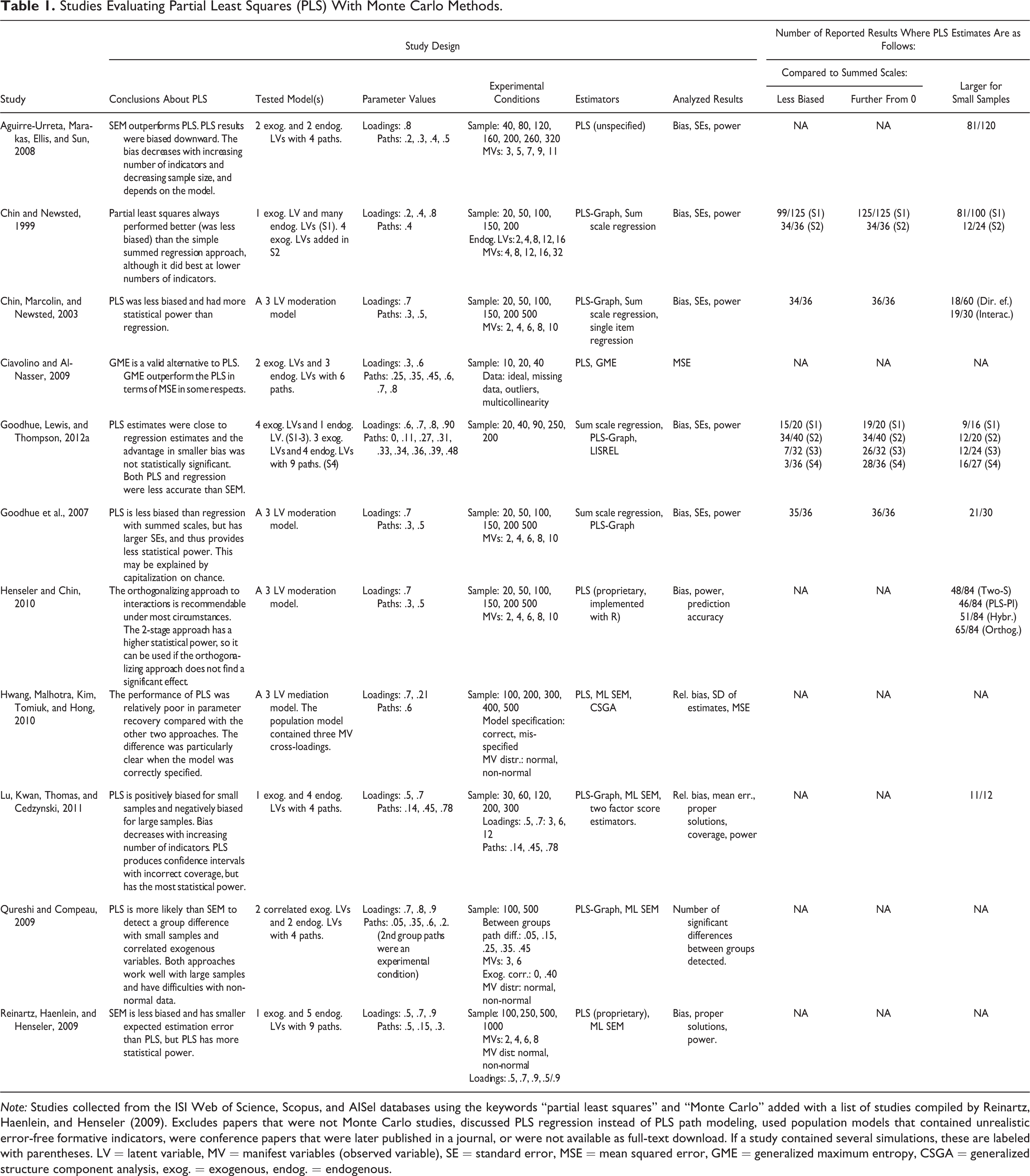
Note: Studies collected from the ISI Web of Science, Scopus, and AISel databases using the keywords “partial least squares” and “Monte Carlo” added with a list of studies compiled by Reinartz, Haenlein, and Henseler (2009). Excludes papers that were not Monte Carlo studies, discussed PLS regression instead of PLS path modeling, used population models that contained unrealistic error-free formative indicators, were conference papers that were later published in a journal, or were not available as full-text download. If a study contained several simulations, these are labeled with parentheses. LV = latent variable, MV = manifest variables (observed variable), SE = standard error, MSE = mean squared error, GME = generalized maximum entropy, CSGA = generalized structure component analysis, exog. = exogenous, endog. = endogenous.

When two latent variables are approximated with composites, the correlation between these approximations will underestimate the true correlation because of the well-known attenuation effect, which depends on the reliability of the approximations (Bollen, 1989, pp. 166-167; Cohen, Cohen, West, & Aiken, 2003, pp. 38-39; Goodhue et al., 2012b). The effects are more complex in multiple regression models, but on average random measurement error causes underestimation of the path coefficients, also in PLS (e.g., Gefen et al., 2011). The smaller bias in PLS estimates has been interpreted earlier as evidence of better reliability of the PLS composites (e.g., Chin et al., 2003), but it will be shown later that this is an incorrect interpretation.

A few of the reviewed papers noticed that there is something peculiar in the PLS estimates. Aguirre-Urreta, Marakas, Ellis, and Sun (2008) note that the PLS estimates tend to get larger when sample size decreases, but could not explain why this happens. Goodhue et al. (2007) noted that when analyzing interaction effects, the PLS estimates of the interaction term seem to be higher than regression with summed scales. They offered capitalization on chance as a possible explanation for this finding, but did neither provide any direct evidence to support this idea nor attempt generalize it outside the interaction effect. Their latest paper (Goodhue et al., 2012b), which is a more general criticism toward PLS, does not discuss capitalization on chance at all. Schermelleh-Engel, Werner, Klein, and Moosbrugger (2010) reinterpreted the data presented by Goodhue et al. (2007) and noted that capitalization on chance may explain the sampling distribution of the interaction effect, but they too do not attempt to generalize the effect outside interactions. Rönkkö and Evermann (2013) discuss the effect of correlated errors on PLS estimates and show that in a simple two-construct case, PLS seems to be sensitive to chance correlations resulting in decreased reliability of the latent variable estimates. While they argue that there is no reason to believe that the findings would not generalize, they too fail to provide direct evidence of capitalization on chance or any evidence of the generalizability of their analysis.

The existing studies listed in Table 1 contain several anomalies that could be explained by capitalization on chance. First, if PLS inflates path coefficients by capitalizing on chance, the PLS estimates should be further from zero than summed scales estimates that have fixed indicator weights and therefore cannot capitalize on chance. The second and third columns from right compare how often the PLS estimates are less biased and how often they were simply larger than summed scales estimates, showing that the latter is more often the case. Moreover, some studies, particularly the study by Chin and Newsted (1999), show results with positive bias in simple regressions. Simply increasing reliability of the composites to overcome the attenuation effect cannot result in this type of results, but the authors fail to note and explain these anomalies. Second, because chance correlations increase with decreasing sample size, the PLS estimates should increase when sample size decreases. I analyzed the result tables of the studies included in Table 1 by counting the number of simulation conditions in which the PLS estimates were larger than in the condition with the next higher sample size. These results are listed in the last column and they show that the effect is present to some extent in all of the studies except in the study by Chin et al. (2003). One possible explanation for this anomaly would be the effect of multicollinearity in their interaction model. This explanation is consistent with the fact that in a later study with the same data generation procedure (Henseler & Chin, 2010), the effect of increasing path estimates is strong when multicollinearity is eliminated through orthogonalization. Third, sometimes there may be a strong chance correlation to the opposite direction of the effect, which should cause the sampling distribution of the PLS estimates have a long tail and a secondary mode on the opposite side of zero. This effect is seen clearly in both of the studies by Goodhue et al. (2007, 2012b) and the study by Rönkkö and Evermann (2013), which are the only reviewed studies that presented any information about the shape of the distribution of the PLS estimates.

Reviewing the existing studies, there seems to be some indirect evidence of PLS capitalizing on chance although it has rarely been interpreted as such. Because the attenuation effect causes the parameters to be underestimated and capitalizing on chance correlations causes bias that is often toward the opposite direction, PLS indeed often has smaller bias than regression with summed scales. However, interpreting this as an advantage, like many of the reviewed studies did, is seriously misguided. The next two sections show how PLS capitalizes on chance correlations between the error terms in a general case and then show direct simulation evidence that this is a very strong effect, which makes PLS unsuitable for any type of statistical inference.

Formal Analysis of How and Why the PLS Method Capitalizes on Chance Correlations

The PLS weights and therefore also the path estimates are completely determined by the sample covariance matrix (Lohmöller, 1989; Rönkkö, 2013), which is a sample realization of the population covariance matrix of the indicator variables. For a common factor model, the population covariance matrix of the indicators is (cf., Bollen, 1989, p. 35):

Σ = {Λ Φ Λ}^{^{'}} + Θ,

where Λ is a (p × n) matrix of factor loadings, Φ is a (n × n) covariance matrix of the latent variables, and Θ is the covariance (p × p) matrix of the error terms, where n is the number of latent variables and p is the number of indicators. Because the PLS model does not allow cross-loadings or correlations between error terms, I will only focus on the case where these assumptions hold in the population. Even in this case, the sample covariance matrix of the indicators, S, is never identical to the population covariance matrix Σ because of sampling variability, but approaches Σ when the sample size increases. In SEM this does not pose problems because the assumption about correct model pertains only to the population model, and it is explicitly acknowledged that the sample covariance matrix is different from the population covariance matrix and this discrepancy follows the χ² distribution after adjusting for sample size. Although it is commonly believed that PLS has less stringent assumptions than SEM, this is incorrect in the case of correlations between the error terms. The assumption that PLS makes is that the residuals are uncorrelated (Wold, 1982) and because residuals are sample realizations, this implies a much stronger assumption than the population model assumption made in SEM.

As explained earlier, PLS uses weighted composites as approximations for latent variables. The indicators are arranged as indicator blocks so that each block is associated with exactly one composite and each indicator belongs to exactly one block according to a (p × n) matrix of outer weights W. Starting with unit weights, the weights are adjusted iteratively in two steps called inner estimation and outer estimation until convergence. To simplify the equations, I will assume that all the variables, including the latent variables in the population, the observed data, and the calculated composites are always standardized. The correlation matrix between the weighted composites is

r_{C} = W^{'} S W .

During inner estimation, this matrix is used to calculate a (n × n) matrix of inner weights E. The PLS literature describes three alternative inner estimation schemes, but because these have been shown to produce nearly identical results (Noonan & Wold, 1982), I describe only the simplest one, the centroid weighting system. In this scheme the cell E_ij is set to sign of $r_{C_{i j}}$ if two latent variables, η_i and η_j are connected with a regression path in the model, and zero otherwise. This leads to the diagonal of E being always zero.¹ After this, a new set of composite variables are simply sums of the indicators weighted by a product of W and E. During outer estimation we calculate a correlation matrix between the new values of the composite variables and the indicator variables and use these correlations as new weights W. This is called Mode A estimation in the PLS literature and it is commonly used when the population model is assumed to be a common factor model (“reflective” in the PLS terminology).² Because W and E are always scaled so that the resulting composites are standardized, we can write the correlations between the indicators and the composites as:

r_{x C} = S W E,

where $r_{x C}$ is a (p × n) matrix of correlations between indicators and composites. We can substitute S with the sample correlations between observed variables, latent variables, and error terms and rearrange as follows:

r_{x C} = λ ϕ λ^{^{'}} W E + θ W E,

where λ are the sample correlations between indicators and latent variables, φ are the sample correlations between latent variables, and θ are the sample correlations between the error terms. (Some effects of sample correlations between error terms and latent variables are omitted for clarity.) Equation 4 contains two terms, which I call structural effects term and error correlations term. Because the diagonal of E is zero, the correlations between indicators in the same block are ignored and only correlations across indicator blocks are used. In the asymptotic case, θ is a diagonal matrix. Each row of W has exactly one non-zero element and the elements on the diagonal of E are all zero, and therefore all the elements that are non-zero in W are zero in WE. Multiplying WE with a diagonal θ will simply scale each cell of WE with a scalar. As a result, the elements θ that are used in the indicator weighting process are zeros and thus the error correlations term has no impact on the indicator weights in the asymptotic case.

In the structural effects term, the factor loadings λ are multiplied by $ϕ λ^{^{'}} W E$ , which is an n by n matrix. Because there are no cross-loadings, there is exactly one non-zero term on each row of λ in the asymptotic case, which means that each factor loading in an indicator block is scaled with the same scalar. In other words, in the asymptotic case the indicators are weighted proportionally to their factor loadings (Dijkstra, 1981, pp. 55, 73). This is different from principal component weights or the any of the commonly used factor score weights, but is instead a common way to erroneously calculate factor scores (Glass & Maguire, 1966).

In a finite sample, things get more complicated because the correlations between the errors are almost never exactly zero in a sample because of random sampling variations (θ is no longer diagonal). This results in indicators with error correlations in the same direction as the correlation caused by the latent variables receiving higher weights. Because the factor loadings are multiplied by $ϕ λ^{^{'}} W E$ , but correlations between error terms only by WE, one unit difference in error correlations has a much higher impact on the indicator weights than one unit difference in factor loadings. In an extreme case where the latent variables are uncorrelated in the population, the indicator weights are almost completely determined by the off-diagonal elements of θ.

After the indicator weights are calculated, the correlation matrix between the composites, which completely determines the latent variables, is calculated according to Equation 2. Substituting S with the same sample correlations as earlier and rearranging yields:

r_{C} = W^{^{'}} λ ϕ λ^{^{'}} W + W^{^{'}} θ W .

I will again call these two terms structural effects term and error correlations term. The equation shows that if r_C are used as estimates of the correlations between the latent variables (ϕ) there are two sources of error. In the structural effects term the $W^{^{'}} λ$ is a (n × n) matrix of square roots composite reliabilities.³ The product of square roots of two reliabilities is the coefficient of attenuation (cf. Cohen et al., 2003, pp. 55-56), which results in the well-known attenuation effect described earlier.

The second source of error is the error correlations term. When using equal weights, this second source of error increases the variance of the parameter estimates, but because the expected value of each error correlation is zero and they are mutually independent, the expected value of their sum is zero resulting in no bias. With PLS, the effect is different because the indicator weights depend on the error correlations, as shown in Equation 4. Consider again that a population path is positive. In this case, indicators with positive error correlations receive larger weights, and the indicators with negative error correlations receive smaller weights resulting in non-zero expected value and a positive bias in the results.

Monte Carlo Study of the Sampling Distribution of PLS Estimates

The previous described a potential problem in the PLS algorithm but did not address the magnitude of the problem. This section address the severity of the problem with a Monte Carlo simulation. The full R code for the study is included in Appendix 1, available online. Also, a picture is worth a thousand words, and the distribution plots that will soon follow communicate the problem in a much more clear way than the formal analysis presented in the previous section.

Simulation Design

Prior studies have argued that the structure of the estimated model can affect the bias (Aguirre-Urreta et al., 2008; Cassel et al., 2000) and the number of false positives (Goodhue et al., 2012b) in a PLS analysis. Therefore, to avoid capitalizing on idiosyncrasies of one particular model, I chose to generate a new, random population model for each simulation round. These random models consisted of six latent variables with eight paths reflecting typical empirical applications of PLS (Hair, Sarstedt, et al., 2012; Ringle et al., 2012). The path values were randomly set using values –.3, –.2, –.1, .1, .2, and .3 with equal probabilities. The measurement model varied according to the first two experimental factors listed in Table 2. The population values of the factor loadings were set by taking the factor loading based value and adding a random number from uniform distribution [–.1, .1] to each loading to simulate uneven reliability of the indicators. Although the population factor loading of .4 is low, such low values can be mistakenly accepted as reliable measurements because PLS severely overestimates low factor loadings (Rönkkö & Evermann, 2013).

Table 2.

Monte Carlo Simulation Design Factors and Values.

Design Factor	Values
Number of indicators	3, 4, 6
Factor loading base value	.4, .6, .8
Sample size	50, 100, 250
Estimated model	Correct, minor misspecification (1 path removed and 1 added), severe misspecification (4 paths removed and 4 added).

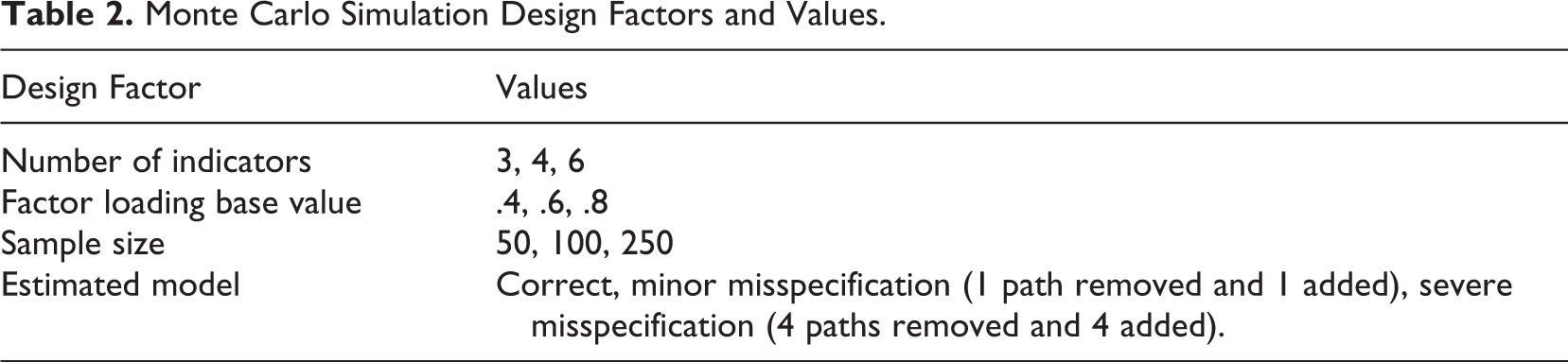
I generated the data by first generating a sample of latent variable true scores by drawing multivariate normal samples using a covariance matrix calculated from the population model. Then I generated the indicator base data by multiplying the latent variable true scores with the factor loadings and used each base data to generate two sets of indicator data. The original data were created by adding error terms drawn randomly from multivariate normal distribution with zero population correlations scaled so that the population variances of the indicators were one. The manipulated data were generated by taking the error terms used in the original data and orthogonalizing them maintaining their variances before adding them to the indicator base data. The manipulated data were thus in all respects identical to the original data with the exception that chance correlations between error terms were artificially removed.

I used each set of original data to estimate three models according to the fourth experimental factors: the correct model, which was identical to the population model, and two misspecified models that were created by removing paths and adding nonexisting paths randomly. This resulted in a full factorial design of 81 cells (3 × 3 × 3 × 3). For each cell, 500 independent replications were used. Each model was estimated with PLS, SEM, and regression analysis with summed scales. The simulation was conducted using the R statistical programming environment (version 2.15.2, R Core Team, 2013) using the plspm package (version 0.3.7, Sanchez & Trinchera, 2013) to for the PLS analysis and lavaan (version 0.5-12, Rosseel, 2012) for the SEM analysis.

Simulation Results

A key argument by the PLS proponents is that the way in which PLS weights the indicators does maximize the reliability of the composites or minimize the effect of random errors (e.g., Chin et al., 2003; Gefen et al., 2011), but there is no direct evidence that this would be the case (Rönkkö & Evermann, 2013). I tested this argument by comparing the squared correlations between the composites and the latent variable true scores that they were approximating. The unweighted summed scales were more reliable in every one of the 81 experimental conditions.

Then I compared the path estimates from these two methods and SEM. The PLS estimates were always less biased and always on average further from zero than estimates from regression with summed scales. The mean squared error (MSE), which measures the inaccuracy of an estimator (i.e., risk, Lehmann & Casella, 1998, pp. 5-7), was statistically significantly higher for PLS in 71 out of 81 conditions. In the remaining 10 conditions MSEs were identical to the third decimal between the methods. Comparing PLS and SEM revealed that SEM was almost always less biased than PLS but had larger MSE, particularly with smaller sample sizes. This result is expected because the ML estimator is inaccurate with small samples (Bollen, 1989). Comparing PLS estimates across conditions revealed that on average, the PLS estimates were further from zero with smaller samples. All these results are consistent with the earlier studies shown in Table 1 and support the argument that PLS capitalizes on chance. The full set of comparison tables is included in Appendix 2.

Figure 2, Figure 3, and Figure 4, showing the distribution of path estimates for PLS, regression with summed scales, and SEM for the cases in which the population parameter is 0 (i.e., no path exists in the population), has an absolute value of .1, or has an absolute value .3, respectively. The purpose of these analyses is not to show that chance correlations have an effect on the PLS weights per se, but to assess the impact that the chance correlations have on the path coefficients when the indicator weights have been calculated with realistic data where chance correlations exists in the sample. The distributions marked with solid lines are calculated using the original data, where the errors were uncorrelated in the population. The second set of results, marked with dashed lines, are calculated using the indicator weights from the analysis using original data but using the manipulated data, where the error terms were orthogonalized in the sample, to calculate the final composites. This is identical to removing the error correlations term from Equation 5 and can therefore be used to analyze how strongly chance correlations affect the results. Because SEM does not use indicator weights, estimating the effect of chance correlations this way was not possible for this method and therefore only one set of results is included for SEM.

Figure 2.

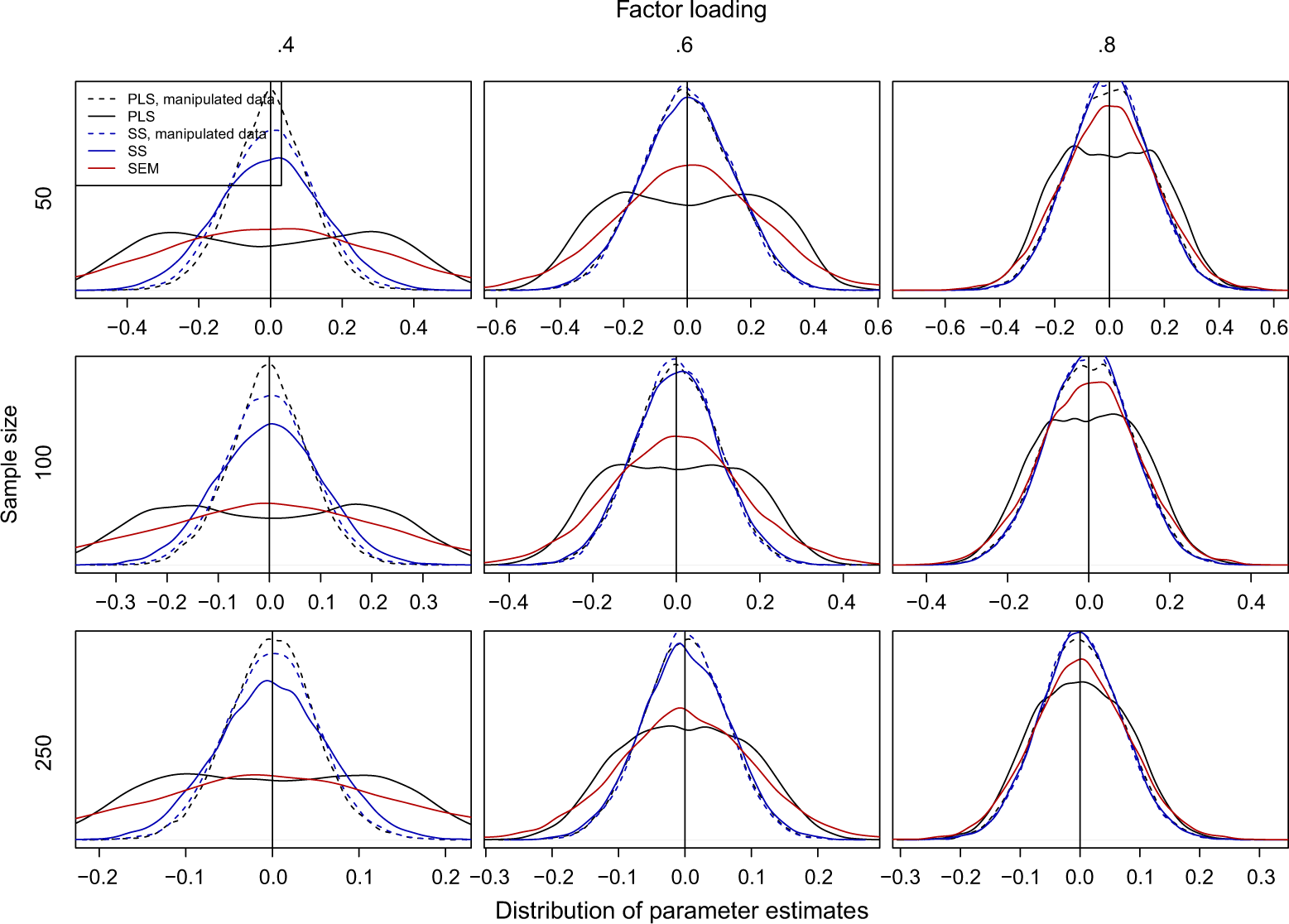
Distribution of the path estimates (kernel density estimates) when the population parameter is 0.

Figure 3.

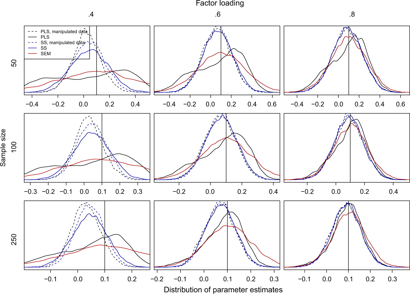
Distribution of the path estimates (kernel density estimates) when the population parameter is .1.

Figure 4.

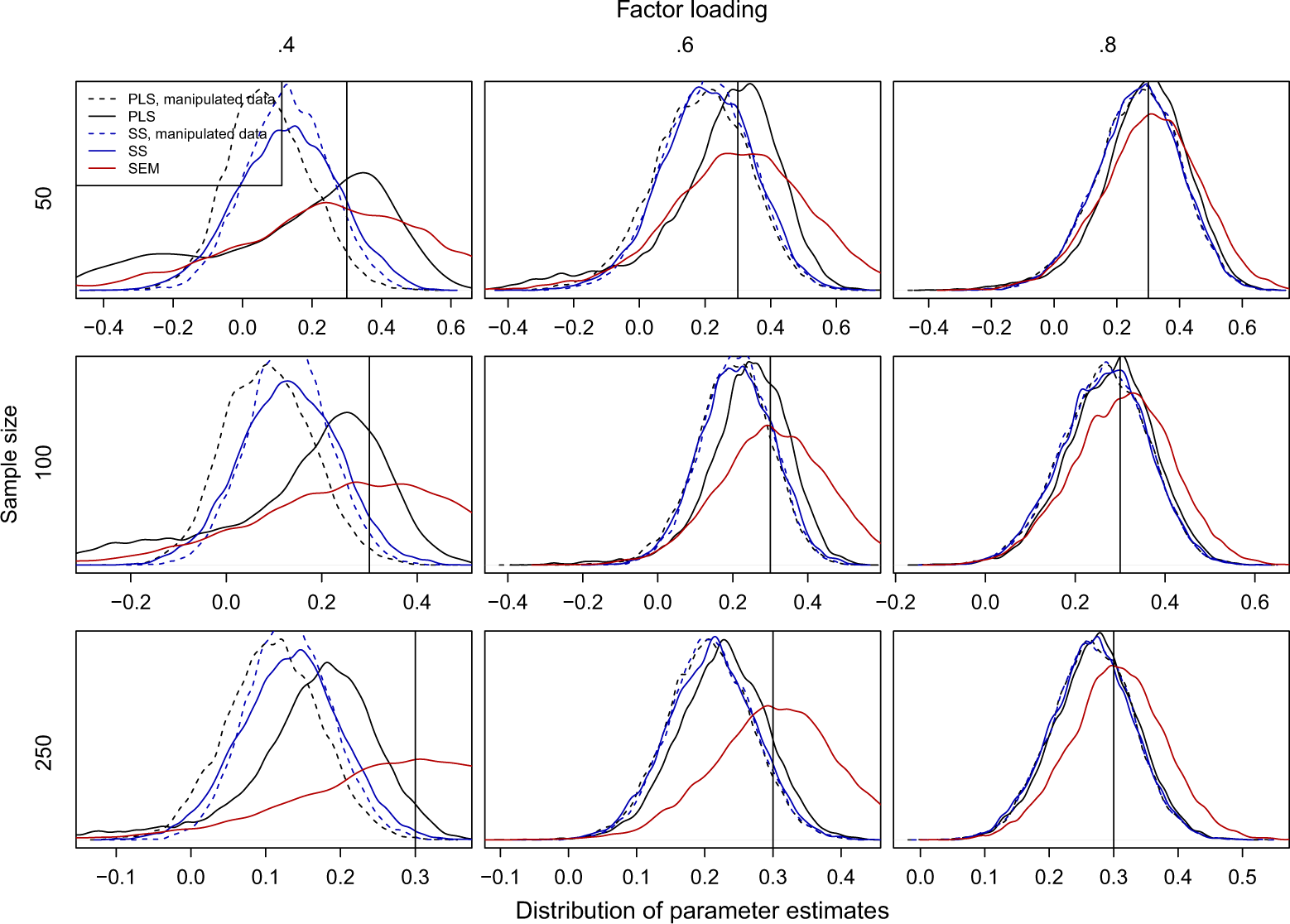
Distribution of the path estimates (kernel density estimates) when the population parameter is .3.

In Figure 2, the PLS estimates and the summed scales estimates are approximately unbiased because they are distributed evenly around zero. For the summed scales, the shape of the distribution is similar for both sets of data, but the variance of the estimates is slightly smaller when chance correlations between errors were removed. This scenario is expected because the error caused by chance correlations has a non-zero variance but has an expected value of zero. In contrast, with PLS composites, the variance of the estimates increases substantially, and the distribution changes into a bimodal form, which resembles the distribution reported for the two latent variable model by Rönkkö and Evermann (2013), but does not follow any known probability distribution. This is very problematic because virtually all current PLS studies use the method for null hypothesis significance testing of the path coefficients comparing the ratio of the parameter estimate and its standard error (t-statistic) with t-distribution. However, because the underlying distribution of parameter estimates is non-normal, the ratio of the parameter estimate and its standard error cannot follow the t-distribution regardless of how the standard error is estimated. Because the t-statistic does not follow the t-distribution, using the t-distribution to obtain a p-value, as is the current practice, is not appropriate (Rönkkö & Evermann, 2013).

Figure 3 and Figure 4 depict the same analysis for paths with an absolute value of .1 or .3 in the population, respectively. In these figures, the PLS estimates are slightly smaller than the summed scale estimates obtained when the effect of chance correlations between the error terms is eliminated from the path coefficients. This is expected because PLS composites were less reliable and the strength of the attenuation effect depends on reliability. With the original data, the effect of the error correlations biasing the PLS estimates away from zero, which was already observed in Figure 2, is again visible. When the true parameter value is small (absolute value is .1), the peak of the distribution is to the right of the true value, meaning that the parameters are mostly overestimated. With the larger population values (absolute value is .3), the peak of the PLS estimates is closer to the population value, but the paths are mostly underestimated. These results show that the widely held belief that PLS underestimates path coefficients (e.g., Chin, 1998) is incorrect because small path coefficients are clearly overestimated.

The figures show that in addition to the well-known attenuation effect, the PLS estimates suffer from also another source of bias that is to the opposite direction and these two sources of bias can in some instances cancel out each other. The question thus becomes is creating a new and thus far unknown source of bias the best way to compensate for the attenuation effect? There are at least three reasons why this is definitely not the case: First, the absolute size of the attenuation effect depends on the true value of the regression path and the factor loadings, whereas the bias caused by the error correlations does not, at least not directly. Second, the correction for attenuation should not depend on the strength of the error correlations, unlike the bias in the PLS results. Third, capitalizing on chance correlations prevents significance testing of path estimates because the sampling distribution of estimates corrected this way is no longer known. The problem of attenuation is well known and we have decades of research on how the bias can be corrected resulting in unbiased estimates without sacrificing the shape of the distribution of the estimates (Charles, 2005; Le, Schmidt, & Putka, 2009; Lu & Thomas, 2008; Muchinsky, 1996; Zimmerman, 2007; Zimmerman & Williams, 1997). I compared the PLS estimates with disattenuated regression estimates confirming that also in these simulation conditions the results from disattenuated regression were substantially less biased than PLS estimates. While the correction for attenuation is a statistically sound approach and has been shown to produce unbiased estimates in fairly general conditions, the resulting estimator is inefficient (Zimmerman & Williams, 1997) and SEM with latent variables has superseded this approach for many practical applications (Cohen et al., 2003, Chapter 12).

Discussion and Conclusions

Like other indicator weighting systems that can be used with regression analysis, PLS suffers from the well-known attenuation problem. In addition to this known problem, this article has showed that PLS suffers from an additional problem of amplifying the effect of chance correlations between error terms. While there is some earlier evidence that PLS does not have the advantages that the proponents of the method argue (e.g., Goodhue et al., 2012b; Rönkkö & Evermann, 2013), the conclusions of these studies have been relatively mild. For example, Goodhue et al. (2012b) concluded their paper by stating that “PLS is still a convenient and powerful technique that is appropriate for many research situations” (p. 999) and Rönkkö and Evermann (2013) merely state that their results cast strong doubts on the usefulness of the method and make it difficult to justify the use of the method.

Understanding the effects of chance correlations on the PLS estimates is also important because the proponents argue that while this may be a problem, it is limited in scope. “Capitalization on chance is indeed an issue, but is mainly limited to very small models with weakly related constructs,” but also continue that “It is pivotal to understand under which conditions this phenomenon occurs” (Rai, Goodhue, Henseler, & Thompson, 2013, p. 2). This paper presents results that hopefully bring about that pivotal understanding: The results show that the apparent advantage of PLS is a fallacy caused by ignoring the effect of chance correlations on the PLS results. These findings also provide an explanation for the positive conclusions about the statistical power of PLS that some studies Table 1 make. Because capitalization on chance makes PLS estimates non-normally distributed, these conclusions may just be results of inappropriate use of the t-test for non-normal data and not reporting false positives when doing so (Rönkkö & Evermann, 2013). It is rather unlikely that anyone would deliberately want to amplify the effect of chance correlations that are idiosyncratic to a sample in their study, particularly when this means also sacrificing the ability to test the statistical significance of the resulting parameter estimates.

The results also show that the existing attempts of fixing PLS by addressing its asymptotic properties and consistency (Dijkstra & Henseler, 2012; Dijkstra, 2014) are unlikely to succeed as long as they ignore an equally severe problem of amplifying the effect of chance correlations that only manifests in finite samples. The best way to eliminate this effect would be to substitute the model-dependent weighting system with equal weights or factor scores weights. In other words, the best way to fix PLS would be to abandon the PLS indicator weighting method altogether and instead focus improving existing component-based SEM methods that do not share the key weakness of PLS exposed in this paper.

The results raise two important questions: (1) On a higher level of abstraction, why does PLS perform poorly when it is applied to data originating from a common factor model? (2) How has the effect of amplifying chance correlations gone unnoticed for so long? The answer to the first question is that PLS was initially developed with a strong focus on prediction. In fact, in analyzing the work of Wold, the developer of PLS, it is difficult to find any recommendations for using the method for statistical inference. In contrast, Dijkstra, Wold’s student, concluded his dissertation on PLS by specifically recommending against using PLS for statistical inference (Dijkstra, 1981, p. 191). While PLS has been shown to produce construct scores that predict one another better than summed scales (Chin, 2010), prediction ability of a model and construct validity that is important when working with theory are two fundamentally different things (cf. Nunnally, 1978, Chapter 3). Thus, by maximizing prediction, PLS sacrifices construct validity and the ability to do null hypothesis significance testing.

The reason why this effect was not noted earlier is most likely because PLS, although used extensively in some disciplines, has not been extensively studied. For example, in Table 1, all but two studies were published in the past five years, and only three were published in research methods journals, the remainder of which were book chapters and papers in applied disciplines. In fact a review of several current beliefs about the PLS method by Rönkkö and Evermann (2013) indicated that many of the prevalent beliefs about the PLS method fit the definition of methodological myths and urban legends: Instead of being based on known statistical principles or rigorous simulation studies, most papers about the PLS method just repeat what earlier similar papers have stated. The fact that PLS has started to enter some of the mainstream textbooks about statistical analysis (Hair, 2010, Chapter 15; Kline, 2010, pp. 287-288; Rigdon, in press), makes these results that expose a previously unknown flaw in the PLS method even more important and timely.

Footnotes

Author’s Note

The paper is loosely based on a paper presented in the 2010 International Conference on Information Systems. The author wishes to thank Jukka Ylitalo for his valuable help with the early versions of the paper.

Declaration of Conflicting Interests

The author(s) declared no potential conflicts of interest with respect to the research, authorship, and/or publication of this article.

Funding

The author(s) received no financial support for the research, authorship, and/or publication of this article.

Notes

Supplemental Material

Supplementary material for this article is available online at .

References

45 Journals used in FT Research Rank. (2012, February 22). Financial Times. Retrieved from http://www.ft.com/intl/cms/s/2/3405a512-5cbb-11e1-8f1f-00144feabdc0.html

Aguirre-Urreta

M. I.

Marakas

Ellis

Sun

(2008). A Monte Carlo investigation of partial least squares, with implications for both structural and measurement models. AMCIS 2008 Proceedings. Retrieved from http://aisel.aisnet.org/amcis2008/246/

Bentler

P. M.

Huang

(2014). On components, latent variables, PLS and simple methods: Reactions to Ridgon’s rethinking of PLS. Long Range Planning.

Bollen

K. A.

(1989). Structural equations with latent variables. New York, NY: John Wiley & Son Inc.

Cassel

C. M.

Hackl

Westlund

A. H.

(2000). On measurement of intangible assets: A study of robustness of partial least squares. Total Quality Management, 11(7), 897–907. doi:10.1080/09544120050135443

Charles

E. P.

(2005). The correction for attenuation due to measurement error: Clarifying concepts and creating confidence sets. Psychological Methods, 10(2), 206–226. doi:10.1037/1082-989X.10.2.206

Chin

W. W.

(1998). The partial least squares approach to structural equation modeling. In Marcoulides

G. A.

(Ed.), Modern methods for business research (pp. 295–336). Mahwah, NJ: Lawrence Erlbaum Associates Publishers.

Chin

W. W.

(2010). Bootstrap cross-validation indices for PLS path model assessment. In Vinzi

E. V.

Chin

W. W.

Henseler

Wang

(Eds.), Handbook of partial least squares (pp. 83–97). New York: Springer.

Chin

W. W.

Marcolin

B. L.

Newsted

P. R.

(2003). A partial least squares latent variable modeling approach for measuring interaction effects: Results from a Monte Carlo simulation study and an electronic-mail emotion/adoption study. Information Systems Research, 14(2), 189–217.

10.

Chin

W. W.

Newsted

P. R.

(1999). Structural equation modeling analysis with small samples using partial least squares. In Hoyle

R. H.

(Ed.), Statistical strategies for small sample research (pp. 307–342). Thousand Oaks, CA: Sage Publications.

11.

Ciavolino

Al-Nasser

A. D.

(2009). Comparing generalised maximum entropy and partial least squares methods for structural equation models. Journal of Nonparametric Statistics, 21(8), 1017–1036. doi:10.1080/10485250903009037

12.

Cohen

West

S. G.

Aiken

L. S.

(2003). Applied multiple regression/correlation analysis for the behavioral sciences. London: Lawrence Erlbaum Associates.

13.

Dijkstra

T. K.

(1981). Latent variables in linear stochastic models: Reflection on “maximum likelihood” and “partial least squares” methods (Doctoral dissertation). Rijksuniversiteit te Groningen.

14.

Dijkstra

T. K.

(2010). Latent variables and indices: Herman Wold’s basic design and partial least squares. In Vinzi

E. V.

Chin

W. W.

Henseler

Wang

(Eds.), Handbook of partial least squares (pp. 23–46). New York: Spinger.

15.

Dijkstra

T. K.

(2014). PLS’ Janus face. Long Range Planning. doi:10.1016/j.lrp.2014.02.004

16.

Dijkstra

T. K.

Henseler

(2012). Consistent and asymptotically normal PLS estimators for linear structural equations. Working paper. http://www.rug.nl/staff/t.k.dijkstra/research

17.

Dijkstra

T. K.

Schermelleh-Engel

(2013). Consistent partial least squares for nonlinear structural equation models. Psychometrika. doi:10.1007/s11336-013-9370-0

18.

Gefen

Rigdon

E. E.

Straub

(2011). An update and extension to SEM guidelines for administrative and social science research. MIS Quarterly, 35(2), iii–A7.

19.

Glass

G. V.

Maguire

T. O.

(1966). Abuses of factor scores. American Educational Research Journal, 3(4), 297–304. doi:10.2307/1162038

20.

Goodhue

D. L.

Lewis

Thompson

(2007). Statistical power in analyzing interaction effects: Questioning the advantage of PLS with product indicators. Information Systems Research, 18(2), 211–227.

21.

Goodhue

D. L.

Lewis

Thompson

(2012a). Comparing Pls to regression and Lisrel: A response to Marcoulides, Chin, and Saunders. MIS Quarterly, 36(3), 703–A10.

22.

Goodhue

D. L.

Lewis

Thompson

(2012b). Does PLS have advantages for small sample size or non-normal data. MIS Quarterly, 36(3), 981–1001.

23.

Hair

J. F.

(2010). Multivariate data analysis: A global perspective (7th ed.). Upper Saddle River, NJ: Pearson Education.

24.

Hair

J. F.

Ringle

C. M.

Sarstedt

(2012). Partial least squares: The better approach to structural equation modeling? Long Range Planning, 45(5-6), 312–319. doi:10.1016/j.lrp.2012.09.011

25.

Hair

J. F.

Sarstedt

Ringle

C. M.

Mena

J. A.

(2012). An assessment of the use of partial least squares structural equation modeling in marketing research. Journal of the Academy of Marketing Science, 40(3), 414–433. doi:10.1007/s11747-011-0261-6

26.

Hardin

Marcoulides

G. A.

(2011). A commentary on the use of formative measurement. Educational and Psychological Measurement, 71(5), 753–764. doi:10.1177/0013164411414270

27.

Henseler

Chin

W. W.

(2010). A comparison of approaches for the analysis of interaction effects between latent variables using partial least squares path modeling. Structural Equation Modeling: A Multidisciplinary Journal, 17(1), 82–109. doi:10.1080/10705510903439003

28.

Henseler

Dijkstra

Sarstedt

Ringle

Diamantopoulos

Straub

… Calantone

(2014). Common beliefs and reality about PLS: Comments on Rönkkö & Evermann (2013). Organizational Research Methods, 17(2), 182–209.

29.

Hwang

Malhotra

N. K.

Kim

Tomiuk

M. A.

Hong

(2010). A comparative study on parameter recovery of three approaches to structural equation modeling. Journal of Marketing Research (JMR), 47(4), 699–712. doi:10.1509/jmkr.47.4.699

30.

Kline

R. B.

(2010). Principles and practice of structural equation modeling (3rd ed.). New York, NY: Guilford Press.

31.

Schmidt

F. L.

Putka

D. J.

(2009). The multifaceted nature of measurement artifacts and its implications for estimating construct-level relationships. Organizational Research Methods, 12(1), 165–200. doi:10.1177/1094428107302900

32.

Lehmann

Casella

(1998). Theory of point estimation. New York, NY: Springer.

33.

Liang

Saraf

Xue

(2007). Assimilation of enterprise systems: The effect of institutional pressures and the mediating role of top management. MIS Quarterly, 31(1), 59–87.

34.

Lohmöller

J. B.

(1989). Latent Variable Path Modeling With Partial Least Squares. New York, NY: Physica-Verlag.

35.

I. R. R.

Kwan

Thomas

D. R.

Cedzynski

(2011). Two new methods for estimating structural equation models: An illustration and a comparison with two established methods. International Journal of Research in Marketing, 28(3), 258–268. doi:10.1016/j.ijresmar.2011.03.006

36.

I. R. R.

Thomas

D. R.

(2008). Avoiding and correcting bias in score-based latent variable regression with discrete manifest items. Structural Equation Modeling: A Multidisciplinary Journal, 15(3), 462–490. doi:10.1080/10705510802154323

37.

Marcoulides

G. A.

Chin

W. W.

Saunders

(2012). When imprecise statistical statements become problematic: A response to Goodhue, Lewis, and Thompson. MIS Quarterly, 36(3), 717–728.

38.

McIntosh

C. N.

Edwards

J. R.

Antonakis

Reflections on partial least squares path modeling. Organizational Research Methods, 17(2), 210–251.

39.

Mosier

C. I.

(1943). On the reliability of a weighted composite. Psychometrika, 8(3), 161–168. doi:10.1007/BF02288700

40.

Muchinsky

P. M.

(1996). The correction for attenuation. Educational and Psychological Measurement, 56(1), 63–75. doi:10.1177/0013164496056001004

41.

Noonan

Wold

(1982). PLS path modeling with indirectly observed variables. In Joüreskog

Wold

(Eds.), Systems under indirect observation: Causality, structure, prediction. Amsterdam: North-Holland.

42.

Nunnally

(1978). Psychometric theory. New York, NY: McGraw-Hill.

43.

Peng

D. X.

Lai

(2012). Using partial least squares in operations management research: A practical guideline and summary of past research. Journal of Operations Management, 30(6), 467–480. doi:10.1016/j.jom.2012.06.002

44.

Qureshi

Compeau

(2009). Assessing between-group differences in information systems research: A comparison of covariance- and component-based SEM. MIS Quarterly, 33(1), 197–214.

45.

R Core Team. (2013). R: A language and environment for statistical computing. Vienna, Austria: R Foundation for Statistical Computing. Retrieved from http://www.R-project.org/

46.

Rai

Goodhue

D. L.

Henseler

Thompson

(2013). To PLS or not to PLS: That is the question. AMCIS 2013 Proceedings. Retrieved from http://aisel.aisnet.org/amcis2013/Panels/PanelSubmissions/2

47.

Reinartz

W. J.

Haenlein

Henseler

(2009). An empirical comparison of the efficacy of covariance-based and variance-based SEM. International Journal of Research in Marketing, 26(4), 332–344. doi:10.1016/j.ijresmar.2009.08.001

48.

Rigdon

E. E.

(2013). Partial least squares path modeling. In Hancock

G. R.

Mueller

R. O.

(Eds.), Structural equation modeling: A second course (2nd ed.). Charlotte, NC: Information Age.

49.

Ringle

C. M.

Sarstedt

Straub

D. W.

(2012). A critical look at the use of PLS-SEM in MIS Quarterly . MIS Quarterly, 36(1), iii–xiv.

50.

Rönkkö

(2013). matrixpls: Matrix-based partial least squares estimation. Retrieved from http://cran.r-project.org/web/packages/matrixpls

51.

Rönkkö

Evermann

(2013). A critical examination of common beliefs about partial least squares path modeling. Organizational Research Methods, 16(3), 425–448. doi:10.1177/1094428112474693

52.

Rosseel

(2012). lavaan: An R package for structural equation modeling. Journal of Statistical Software, 48(2), 1–36.

53.

Sanchez

Trinchera

(2013). plspm: Tools for partial least squares path modeling. Retrieved from http://cran.r-project.org/web/packages/plspm/index.html

54.

Savalei

Bentler

P. M.

(2007). Structural equation modeling. In Grover

Vriens

(Eds.), The handbook of marketing research: Uses, misuses, and future advances (pp. 330–364). Thousand Oaks, CA: Sage Publications.

55.

Schermelleh-Engel

Werner

C. S.

Klein

A. G.

Moosbrugger

(2010). Nonlinear structural equation modeling: Is partial least squares an alternative? Asta-Advances in Statistical Analysis, 94(2), 167–184. doi:10.1007/s10182-010-0132-3

56.

Tenenhaus

(2008). Component-based structural equation modelling. Total Quality Management, 19(7-8), 871–886.

57.

Treiblmaier

Bentler

P. M.

Mair

(2011). Formative constructs implemented via common factors. Structural Equation Modeling: A Multidisciplinary Journal, 18(1), 1–17. doi:10.1080/10705511.2011.532693

58.

Wold

(1982). Soft modeling—The basic design and some extensions. In Jöreskog

K. G.

Wold

(Eds.), Systems under indirect observation: Causality, structure, prediction (pp. 1–54). Amsterdam, NY: North-Holland.

59.

Zimmerman

D. W.

(2007). Correction for attenuation with biased reliability estimates and correlated errors in populations and samples. Educational and Psychological Measurement, 67(6), 920–939. doi:10.1177/0013164406299132

60.

Zimmerman

D. W.

Williams

R. H.

(1997). Properties of the Spearman correction for attenuation for normal and realistic non-normal distributions. Applied Psychological Measurement, 21(3), 253–270. doi:10.1177/01466216970213005

Supplementary Material

Please find the following supplemental material available below.

For Open Access articles published under a Creative Commons License, all supplemental material carries the same license as the article it is associated with.

For non-Open Access articles published, all supplemental material carries a non-exclusive license, and permission requests for re-use of supplemental material or any part of supplemental material shall be sent directly to the copyright owner as specified in the copyright notice associated with the article.

0.00 MB

0.09 MB

1.26 MB