Count-Based Research in Management

Abstract

We review 11 years (2001-2011) of management research using count-based dependent variables in 10 leading management journals. We find that approximately one out of four papers use the most basic Poisson regression model in their studies. However, due to potential concerns of overdispersion, alternative regression models may have been more appropriate. Furthermore, in many of these papers the overdispersion may have been caused by excess zeros in the data, suggesting that an alternative zero-inflated model may have been a better fit for the data. To illustrate the potential differences among the model specifications, we provide a comparison of the different models using previously published data. Additionally, we simulate data using different parameters. Finally, we offer a simplified decision tree guideline to improve future count-based research.

Keywords

Poisson negative binomial overdispersion zero-inflated simulation

In management research it is often valuable to use dependent variables that count the number of times that an event has occurred. For example, the number of patents that a company has obtained (Penner-Hahn & Shaver, 2005), the number of suggestions an employee makes to their boss (Ohly, Sonnentag, & Pluntke, 2006), or the number of product innovations (Un, 2011)—all of which are important outcomes that may yield insight into future research. Certainly, the ability to estimate the number of times critical events occur is important since it allows for theories to be empirically tested and in turn allows for theories and their constructs to develop (Miller & Tsang, 2011).

However, using a count-based dependent variable often means that scholars must use more specialized models based on Poisson or iterations of the Poisson model. This is because the application of a linear regression model (LRM) is inappropriate for data with a count-based dependent variable (Cameron & Trivedi, 1998) and can result in inefficient, inconsistent, and biased regression models (Long, 1997). Consequently, the use of count-based regression models is increasingly common in management research. In our review of 10 leading management journals—Academy of Management Journal, Administrative Science Quarterly, Journal of Applied Psychology, Journal of International Business Studies, Journal of Organizational Behavior, Journal of Management, Organizational Behavior and Human Decision Process, Organization Science, Personnel Psychology, and Strategic Management Journal—we found that count-based dependent variables were used in 164 papers during the past decade (from 2001 to 2011).

Past surveys have shown that management researchers receive limited training in statistical analysis during their doctoral studies (Shook, Ketchen, Cycyota, & Crockett, 2003, p. 1235). Therefore, it is crucial that our exemplar journals feature both the most accurate and rigorous methodology that can be used to explain a phenomenon—since training in some doctoral programs may be insufficient (Bettis, 2012). While Poisson is generally more appropriate for count-based dependent variables than LRMs, the most basic Poisson regression model has defining characteristics specifying that the dependent variable’s variance equals the mean (Cameron & Trivandi, 1998). This key assumption of the basic Poisson regression model is referred to as equidispersion (Greene, 2003; Long, 1997). Greene (2008) directly notes that “observed data will almost always display pronounced overdispersion” (p. 586). Accordingly, alternative Poisson-based models (e.g., negative binomial, zero-inflated Poisson, zero-inflated negative binomial) are often recommended since equidispersion rarely exists in practice.

Hoetker and Agarwal (2007) propose that when the ratio of the standard deviation exceeds 130% of the mean, overdispersion is likely a problem. In our review of 164 papers using count-based regressions, 49 papers used Poisson-based models, 39 of which used the most basic Poisson, and the rest used panel Poisson. Out of these 39 papers, we found that 85% of them exceeded the 1.30 suggested ratio with an overall average ratio of 2.86, suggesting potential problems related to overdispersion. Moreover, most of these papers did not explicitly mention whether they compared their results with alternative regression analysis such as the negative binomial regression or other more advanced specifications such as the zero-inflated Poisson or zero-inflated negative binomial.

While it is uncertain if these papers’ findings would change with alternative models, failure to address overdispersion can sometimes have important implications (which we will later illustrate with replicated examples, along with a simulation). For example in the worst case scenarios, misspecification can cause independent variables’ significance levels to change, or even worse—the coefficients’ signs may reverse (Allison & Waterman, 2002). By directly illustrating the consequences of failing to address overdispersion and other problems found in count data such as when the data contain an abundance of zeros, our paper offers a framework to help future management researchers (and reviewers) identify the best model to use when estimating regressions on count-based dependent variables. In doing so, our paper addresses four issues: (1) commonly used count-based models, (2) problems related to overdispersion, (3) the importance of dealing with excess zeros, and (4) a guideline that researchers may use to improve their methodology when choosing topics that have a focus on the count of a particular phenomenon occurring. In the following section we provide an overview of the Poisson and negative binomial models.

Commonly Used Count-Based Models

Dependent variables that measure the count of the number of times an event occurs are quite common in management research. For example, scholars may be interested in understanding the frequency of harassment in the workplace (Berdahl & Moore, 2006), or a scholar may be concerned with the number of alliances that a firm has formed (Park, Chen, & Gallagher, 2002). Indeed, the overall use of count-based dependent variables appears to be on an upward trend in recent years, as shown in Figure 1 (growing from just 8 articles in 2001 to a peak of 28 articles in 2010).

Figure 1.

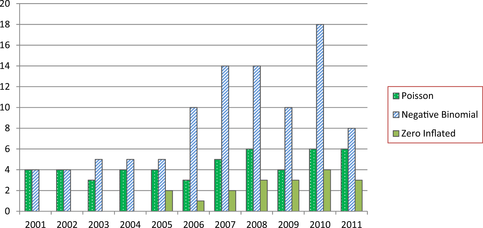
Trend of count-based papers in exemplar management journals (164 total).

The descriptive findings presented in Table 1 are helpful in revealing the common methodological approaches used in estimating regressions with count-based data. Approximately 30% of management scholars used Poisson-based approaches (24% used the most basic Poisson), whereas 59% used models related to the negative binomial distribution, and 11% of the models published in the journals we reviewed used either the negative binomial or Poisson zero-inflated models. As previously noted, the Poisson regression model makes the strong assumption of equidispersion structured as follows:

Equidispersion : var (Y) = E (Y) = μ .

Table 1.

Use of Count-Based Regressions by Journal (2001-2011).

Journals	Poisson^a	Mean to Standard Deviation Ratio (average %)	Negative Binomial	Zero-Inflated Models	Total Papers
Academy of Management Journal	9	270	20	6	35
Administrative Science Quarterly	5	573	19	3	27
Journal of International Business Studies	4	235	13	1	18
Organization Science	2	300	12	2	16
Strategic Management Journal	14	290	19	5	38
Journal of Applied Psychology	6	243	5	0	11
Personnel Psychology	2	106	2	0	4
Journal of Management	1	280	2	0	3
Journal of Organizational Behavior	3	296	3	1	7
Organizational Behavior and Human Decision Processes	3	158	2	0	5
Total (percentage)	49 (30%)	275	97 (59%)	18 (11%)	164
American Sociological Review	5 (17%)	204	19 (63%)	6 (20%)	30

^aThirty-nine of these 49 used the most basic Poisson methodology, with an average mean to standard deviation ratio of 2.86.

The stringent assumption of equidispersion has led some to argue that the most basic Poisson regression model is unreasonable. For example, Kennedy (2003) directly notes that these assumptions are “thought to be unreasonable since contagious processes typically cause occurrences to influence the probability of future occurrences, and the variance of the number of occurrences usually exceeds the expected number of occurrences” (p. 264). This problem alludes to the issue of overdispersion. Dispersion can result from missing variables, interaction terms, the existence of large outliers, or positive correlation among the observations, and so on. Failure to properly address such issues may lead to biased results, and one commonly used model in order to remedy overdispersion is the negative binomial model.

The negative binomial regression model can be viewed as an extension of Poisson since it has the same mean structure as Poisson but adds a parameter to allow for overdispersion. Specifically, data y ₁, … , y_n that follow a negative binomial distribution, neg-bin(α,β), are equivalent to Poisson observations with rate parameters λ₁, … , λ _n that follow a gamma(α,β) distribution. The variance of the negative binomial is: $\frac{β + 1}{β} \frac{α}{β}$ , which is always larger than its mean $\frac{α}{β}$ , in contrast to the Poisson, whose variance is equal to its mean (Gelman et al., 2013). In the limit, as β approaches ∞, the gamma distribution approaches a spike (i.e., all of the probability is associated with a single point and zero elsewhere), and the negative binomial therefore approaches the Poisson, with rate parameter equal to the spike in the underlying gamma distribution (Gelman et al., 2013). That is, the gamma distribution underlying the different Poisson parameters in the mixture only allows for a single parameter value, and so the mixture of Poissons converges to a single Poisson.

Zero-Inflated Models

While the negative binomial is generally a good fit for dealing with overdispersion relative to Poisson, another important potential cause of overdispersion can be due to data with excessive zeros. For example, Wang, Liu, Zhan, and Shi (2010) study how work conflict leads to the number of alcoholic drinks consumed and specifically note that their data have excessive zeros, since work conflict may not necessarily lead to alcohol consumption. Similarly, a researcher may be interested in counting the number of acquisitions a firm makes in a year (Lin, Peng, Yang, & Sun, 2009). However, some firms may not make an acquisition in a given year or even over multiple years. On the other hand, other firms in the data may have an acquisition-based strategy that leads to a wave of acquisitions (Haleblian, McNamara, Kolev, & Dykes, 2012). Due to the simultaneous combination of data having a relatively high frequency of firms with zero acquisitions and firms with acquisitions in waves, overdispersion may arise.

When there are excessive zeros found in the data, alternative models to the negative binomial and Poisson may be appropriate. Specifically, zero-inflated models, both the zero-inflated Poisson (for a recent example, see Pe’Er & Gottschlag, 2011) and the zero-inflated negative binomial (for recent examples, see Corredoira & Rosenkopf, 2010; Soh, 2010), offer potential remedies for dealing with excessive zeros. Despite the benefits of using these models, the use of zero-inflated models is only recently starting to gain traction in management research. Indeed, it is relatively easy to fit these models with cross-sectional data and test the models’ assumptions in popular statistical software such as R, SAS, and STATA.

Our review showed that only a small percentage of management scholars (11%) used such models. Due to the predominate standard of displaying just the mean and standard deviation in the descriptive statistics table, it was difficult to ascertain exactly how many papers may have excess zeros, and unlike Wang et al. (2010), most papers did not directly note the underlying data’s characteristics. Of the few papers reporting zero-inflated models, one paper noted that nearly 90% of the observations had a value of zero (Chang, Chung, & Mahmood, 2006), whereas another paper with just 7% of the observations taking a value of zero found that the zero-inflated model provided a better fit than the more basic underlying Poisson or negative binomial (Antonakis, Bastardoz, Liu, & Schriesheim, 2014).

Moreover, it is important to emphasize that changes from the most basic Poisson to zero-inflated models can be drastic. To help demonstrate the extent of the difference between results, we use data published in Antonakis et al.’s (2014) study aiming to understand why articles are cited. Their paper is an exemplary model for researchers, and it utilizes the zero-inflated negative binomial specification. Additionally, they not only note the level of zeros (7%) but also clearly specify which variable they use to predict the zero inflation in their data, namely, article age. When using zero-inflated methodology, software such as STATA allows the user to specify which variables may be related to the zero observations.

In our review, most of the papers using zero-inflated models did not specify whether they used any variables to predict the zero inflation or they just allowed the constant to be adjusted (the default option in STATA). Accordingly, this is an area where future research may be improved, as specifications may provide a better fit when accounting for specific variables germane to the excess zeros. In Table 2, we use the data from Antonakis and colleagues (2014) to illustrate what the results of their zero-inflated negative binomial analysis would have looked like had they used the most basic Poisson estimation. Table 2 compares the results of the basic Poisson model with those of their zero-inflated negative binomial.

Table 2.

Changes From Basic Poisson to Zero-Inflated Negative Binomial (N = 776).

Variables	Basic Poisson		Δ in Level of Significance	Δ in Sign	Zero-Inflated Negative Binomial
Number of authors	0.04***	(8.56)	YES	NO	0.09**	(3.18)
Article age (a)	–0.04***	(6.32)	YES	NO	–0.05	(1.38)
Cited references	0.01***	(42.34)	NO	NO	0.01***	(5.47)
Quantitative	0.46***	(16.16)	YES	NO	0.35**	(2.95)
Theory	0.48***	(16.50)	YES	NO	0.33*	(2.59)
Review	0.68***	(21.23)	YES	NO	0.52**	(2.78)
Comment/discussion	–0.25***	(4.48)	YES	NO	–0.12	(0.57)
Method	0.59***	(10.30)	YES	NO	0.58*	(2.30)
Agent simulation	–0.51*	(2.41)	YES	NO	–0.51^†	(1.70)
Author cites	–0.00*	(2.42)	YES	YES	0.00^†	(1.74)
Author articles	0.00***	(7.81)	YES	YES	–0.00	(0.86)
Affiliation rank	0.00***	(8.54)	YES	NO	0.00*	(2.08)
Number of articles published (b)	–0.04***	(31.47)	NO	NO	–0.04***	(8.62)
(a) × (b)	0.01***	(45.60)	NO	NO	0.01***	(7.15)
Constant	1.96***	(15.16)	NO	NO	1.89***	(4.01)

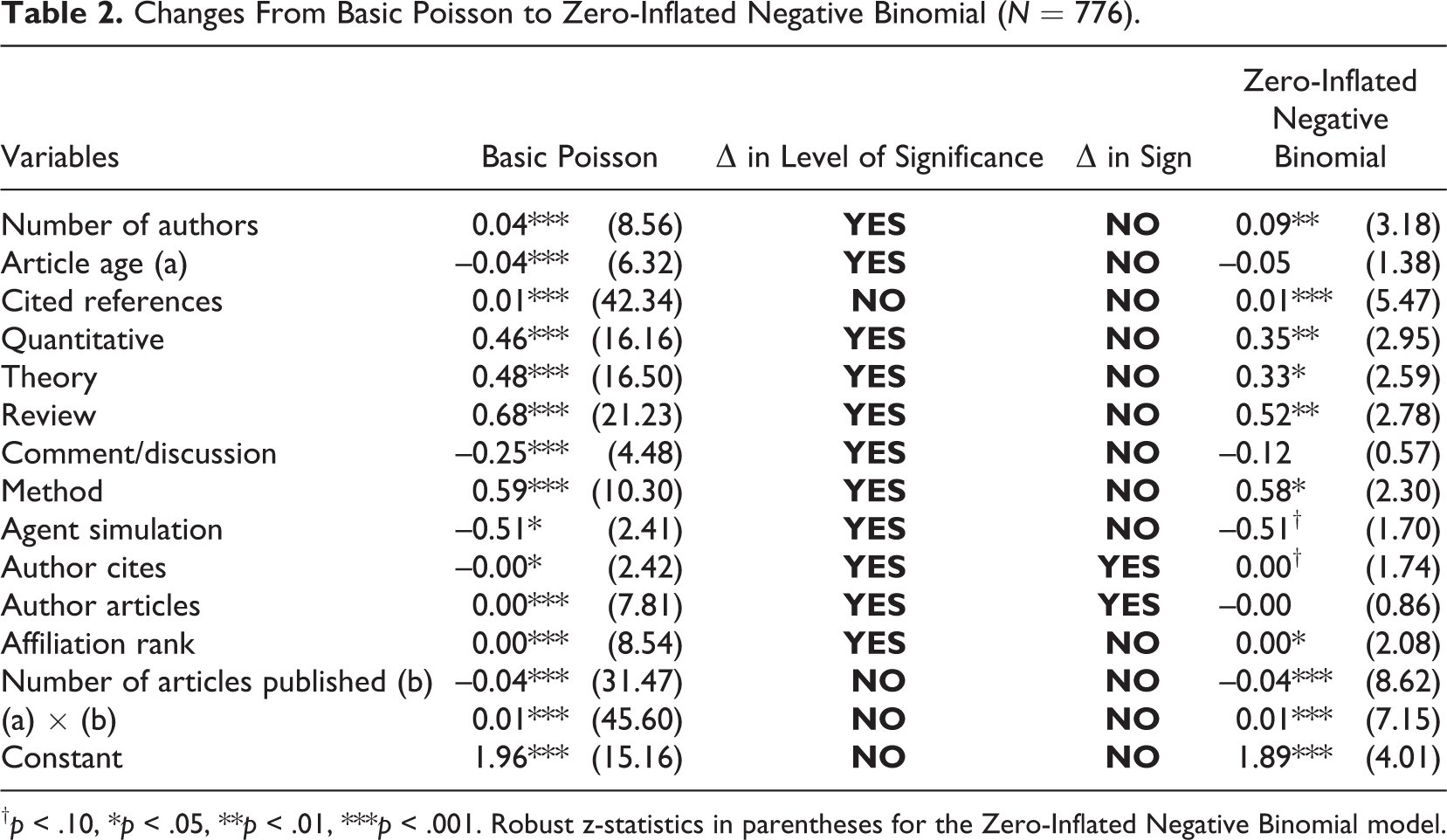
^† p < .10, *p < .05, **p < .01, ***p < .001. Robust z-statistics in parentheses for the Zero-Inflated Negative Binomial model.

Table 2 shows that 11 out of 15 variables experienced a change in their level of significance, with each of the 11 changes resulting in a decline in their level of significance when specifying the zero-inflated negative binomial. Furthermore, in 2 cases, the direction of the coefficient’s sign reverses when using the better fitting zero-inflated model that accounts for the excess zeros found in the data. These findings help underscore the importance of exploring and understanding alternative models when underlying count-based data have strong characteristics leading to overdispersion, such as excessive zeros.

Panel Count Data

Longitudinal analysis with panel data is commonly used. This is because scholars may want to study potential developments over time, such as the effects of work conflict on alcohol consumption over years. Panel data permits more types of individual heterogeneity, which is particularly valuable in the study of organizations over time. Another advantage is that panel data can allow for estimation of Poisson rates for each sampling unit, which may allow the basic Poisson to fit what might otherwise appear to be overdispersed data (Gelman & Hill, 2007). In general, the standard methods of fixed effects versus random effects (and their assumptions) designed for panel data in linear regression models extend to Poisson regression models (Cameron & Trivedi, 1998). Furthermore, the pros and cons associated with fixed and random effects are also quite similar to those identified in linear regression models, with one key difference that the individual specific effects in Poisson regression models are multiplicative rather than additive (Cameron & Trivedi, 1998).

Hausman, Hall, and Griliches’s (1984) study is probably the most well-known and earliest paper to use panel data on a count-based dependent variable for investigating the relationship between past research and development (R&D) expenditures and the subsequent number of patents awarded. Their paper specifically addressed the issues regarding the use of fixed effects versus random effects in their panel of patents awarded and used a conditional likelihood method for negative binomial regression that is now widely used and readily available in popular statistical software such as STATA and SAS. However, some scholars have argued that this model allows for individual-specific variation in the dispersion parameter rather than in the conditional mean (Allison & Waterman, 2002). This means that time-invariant covariates can get non-zero coefficient estimates for those variables, and these covariates are often statistically significant. Indeed, there is a significant debate surrounding the best practices within panel-based count data, and often in practice there is less of a clear cut decision for which of the two effects to use—and in some cases, such as Soh (2010), researchers may find no systematic difference between the two approaches.

Within the broader approach of fixed effects versus random effects, the three most common methods for analyzing count-based data are maximum likelihood, conditional maximum likelihood, and dynamic models. Of the three, the maximum likelihood method is often considered the simplest (Cameron & Trivedi, 1998). However, if the number of observations is small, this model may not be easily estimated. Increasingly popular are dynamic panel count models. Dynamic models introduce dependence over time and can be applied to both random and fixed effects. While there are advocates for both fixed and random effects models, overall, the decision needs to be made on a case-by-case basis. That said, the fixed effects model is generally preferred in cases where conclusions need to be made on the sample, but where overall populations are studied (often not the case in management research), random effects models may be more appropriate.

The primary focus of our paper is to address the more germane issues of overdispersion and excess zeros. As with linear data, the choice of random versus fixed effects is idiosyncratic to the underlying data, so there is no clear recommendation for one or the other. It is important to note that while panel Poisson and negative binomial extensions are widely available in statistical software packages, zero-inflated extensions are not generally available for panel data. As a result, generally the negative binomial distribution is recommended for panel count data, but some have argued that the Poisson distribution is less problematic in a panel setting.¹

In sum, there are different types of models that can deal with count-based variables, in cross-sectional or longitudinal studies. Overdispersion can arise due to different reasons ranging from sampling problems to excessive zeros. Fortunately, there are ways to address problems of overdispersion—and there are also ways to subsequently confirm which models provide a better fit for the data (Vuong, 1989). In the following section we replicate early published data with the aforementioned approaches using corporate interlock data from Ornstein’s (1976) study of Canadian board and executives. It should be noted that only recently are zero-inflated panel models being estimated, due to the complex computation process.

Corporate Interlocks: An Example of Different Count-Based Specifications

In order to show how results may change with different regression models, we use an example that is an extension of the data presented in Fox and Weisberg (2009)—namely, Ornstein’s (1976) study of director interlocks among major Canadian firms. We demonstrate fitting the aforementioned models to the freely available data, from the car package (Fox & Weisberg, 2009, who use it in examples for Poisson and negative binomial regression) in R (R Development Core Team, 2013) and also as STATA download.²

The mean number of interlocks is 13.58, and the standard deviation is 16.08. Accordingly, the ratio of the standard deviation to the mean is just 1.18, which is below the threshold noted by Hoetker and Agarwal (2007) and also below the average ratio of the past papers that used Poisson in our review.

The variables presented in the study fall within the two broad categories, nations and industries. We first fit a standard Poisson regression model, predicting interlocks from log-assets, nations (Canada [base level], UK, US, and other), and industry sector (agriculture base level). All models are significant at p < .001. As shown in Table 3 the variables assets, the nations of the UK and US, and sectors MIN and WOD are all highly significant (p < .001), and the sector CON is also significant at the p < .05 level. If such variables were of interest to our underlying hypotheses we would have strong results—of course assuming that the signs were in the direction we hypothesized. Such strong results may also allow additional control variables suggested by reviewers to enter the model without much effect on our key independent variables of interest. Despite a ratio lower than Hoetker and Agarwal’s (2007) 1.30 threshold, the dependent variable does not meet the assumption of equidispersion. Accordingly, it would be important to at least reestimate the model with the negative binomial regression model as well (Hess & Rothaermel, 2011).

Table 3.

Regressions on the Ornstein Data (N = 100).

	Basic Poisson		Negative Binomial		Zero-inflated Poisson		Zero-Inflated Negative Binomial
Variables	Model I		Model II		Model III		Model IV
(Intercept)	–0.84***	(0.14)	–0.83*	(0.38)	–0.35*	(0.14)	–0.28	(0.35)
log2(assets)	0.31***	(0.01)	0.32***	(0.04)	0.27***	(0.01)	0.27***	(0.03)
nationOTH	–0.11	(0.07)	–0.10	(0.23)	–0.06	(0.08)	0.02	(0.21)
nationUK	–0.39***	(0.09)	–0.39^†	(0.24)	–0.41***	(0.09)	–0.42*	(0.21)
nationUS	–0.77***	(0.05)	–0.79***	(0.13)	–0.69***	(0.05)	–0.69***	(0.12)
sectorBNK	–0.17^†	(0.10)	–0.41	(0.38)	0.06	(0.10)	–0.04	(0.35)
sectorCON	–0.49*	(0.21)	–0.76^†	(0.46)	–0.60**	(0.21)	–0.87*	(0.40)
sectorFIN	–0.11	(0.08)	–0.10	(0.25)	–0.05	(0.08)	–0.04	(0.22)
sectorHLD	–0.01	(0.12)	–0.21	(0.35)	0.05	(0.12)	–0.10	(0.32)
sectorMAN	0.12	(0.08)	0.08	(0.19)	0.22**	(0.08)	0.18	(0.18)
sectorMER	0.06	(0.09)	0.08	(0.23)	0.01	(0.09)	0.01	(0.21)
sectorMIN	0.25***	(0.07)	0.24	(0.19)	0.25***	(0.07)	0.21	(0.17)
sectorTRN	0.15^†	(0.08)	0.10	(0.25)	0.17*	(0.08)	0.09	(0.22)
sectorWOD	0.50***	(0.08)	0.39^†	(0.23)	0.49***	(0.08)	0.39^†	(0.20)
loglikelihood	–1,222		–822		–1,106		–804
df	14		15		28		29

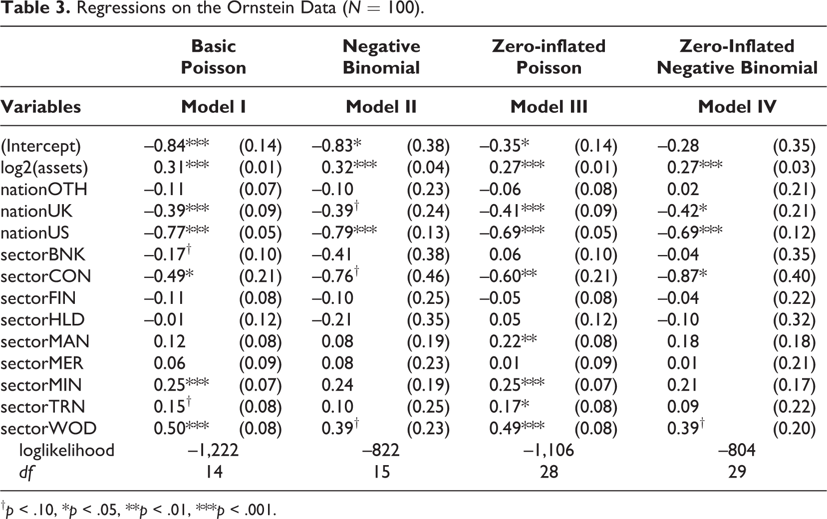
^† p < .10, *p < .05, **p < .01, ***p < .001.

Interestingly, with the negative binomial model (Model II) the results show substantial changes in some of the variables that were previously highly significant in the basic Poisson model. For example, the effect of the nation level variable UK and industry-level variables MIN and WOD have dropped from highly significant (p < .001) to insignificant or marginally significant. Further, the likelihood ratio test of alpha = 0 is significant with the chi-square value of 800, strongly supporting the use of negative binomial over Poisson (p < .001). A nice feature of the nbreg function in STATA is that the Poisson model is already nested within it. Moreover, when estimating the negative binomial model with the STATA nbreg command, if there is no evidence of overdispersion then the results will not vary from the Poisson estimate (Drukker, 2007). As the comparison between Models I and II shows, failure to address overdispersion can have significant consequences for the results of the regressions reported. Despite that the negative binomial is a significantly better fit than the basic Poisson model, there could also be more issues at hand—namely, if there are excess zeros in the data measuring the dependent variable.

In Ornstein’s (1976) data there are 28 zeros, or just over 11% of the data. It would be difficult to know this information unless the author self-discloses it or the reader has past experience with the same or a similar data set. Accordingly, during the review process reviewers should request more information in this area if the authors have not disclosed such information, and we recommend that the nature and the number of zeros found in the data should always be discussed in count-based regressions.

On top of the negative binomial regression, alternative zero-inflated models may be more appropriate.³ The first model that we use to examine whether there is a better fit is the zero-inflated Poisson model. When compared to the basic Poisson model, the results are largely similar except for the sector MAN, which is now significant (p < .01), and the sector BNK, which is not close to being significant anymore but had weak support (p < 0.10) in the basic Poisson model. The sector TRN has also changed from a significance level of p < .10 to p < .05. The Vuong test compares the fit of the zero-inflated Poisson and the basic Poisson models (see STATA guide for details; this test is also available in both R and SAS). In this case, the Vuong test provides strong support (p < .001) that the zero-inflated model is superior to the basic Poisson model.

In addition to the zero-inflated Poisson model, a zero-inflated negative binomial model could also be appropriate for data with overdispersion and many zeros (Corredoira & Rosenkopf, 2010). Zero-inflated negative binomial models are generally more appropriate than their zero-inflated Poisson counterparts when the data display an abundance of zeros and when the likelihood ratio test of alpha = 0 is significant (Long, 1997). Similar to the zero-inflated Poisson, using the Vuong test can help identify whether the model is a better fit compared with the basic negative binomial.

When comparing the results to the basic Poisson model, the findings were very similar to the differences found between the basic negative binomial model and the basic Poisson. However, whereas the UK variable is only significant in the basic negative binomial model at p < .10, and it is now significant at p < .05. The Vuong test suggests that zero-inflated negative binomial is more appropriate than basic negative binomial.

Finally, a useful tool in STATA is the countfit. This command runs all of the aforementioned models and generates a range of statistical tests. It also generates a graph showing the fit of all of the models. We have included the graph from this output in Figure 2.

Figure 2.

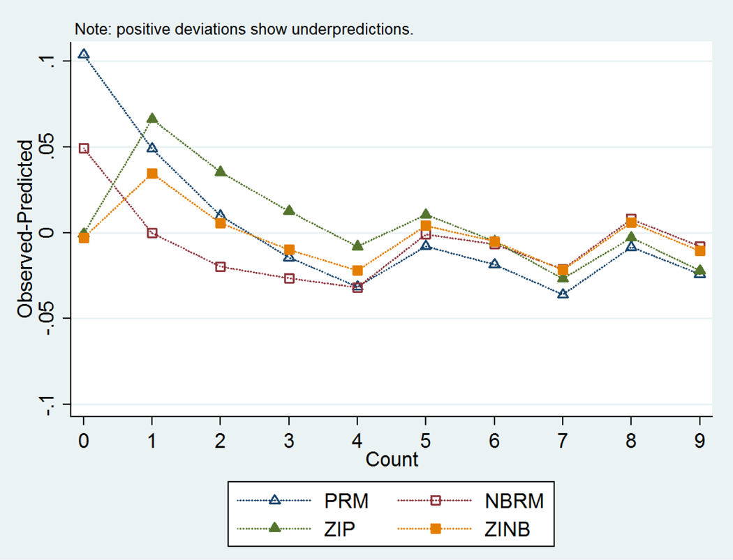
Fit of different models.

The graph shows the deviations from the models’ predictions to the actual data at different counts of interlocks. As expected at zero, both the zero-inflated Poisson and zero-inflated negative binomial provide a much better fit than the basic Poisson and negative binomial. However, when the observation value was a higher count, the predictive values of the basic and zero-inflated models begin to converge. In an effort to help understand when more complex models may be more appropriate, we conducted a Monte Carlo simulation.

A Simulation Study

We conducted a Monte Carlo study to examine the degree of agreement of various different regression models: Poisson, quasi-Poisson,⁴ negative binomial, zero-inflated Poisson, and zero-inflated negative binomial. In every case, the data were generated from a zero-inflated Poisson distribution with mean function:

2.68 + 0.36 X_{1} - 0.001 X_{2} - 0.01 X_{3} - 0.0 X_{4} + 0.08 X_{5} - 0.08 X_{6},

where the predictor variables X _p were drawn from a standard normal distribution. We varied the sample size (250, 500, 1,000), the proportion of zeros (.20, .35, .55), and the variance (6, 10), yielding a set of 18 (3 × 3 × 2) possible combinations. Each Monte Carlo replication was composed of 1,000 trials. Our primary intent here is to demonstrate the fit of the different models to the data and evaluate the basic Poisson regression when the data are overdispersed with excess zeros.

Table 4 provides the primary results of this simulation, which is the mean Vuong statistic across all 1,000 replications comparing the negative binomial (NegBin) model to the Poisson, the zero-inflated Poisson (ZIP) to the negative binomial, and the zero-inflated negative binomial (ZINB) to the ZIP, for each cell of the design. The quasi-Poisson is not included in this table since it does not produce a true likelihood, which is needed to calculate the Vuong statistic. This table shows that for all cells of the design, there is sufficient evidence to reject the Poisson fit at the p < .05 level and to choose the ZINB over the ZIP. Interestingly, when the percentage of zeros is somewhat modest (.20) there is not sufficient evidence, regardless of sample size, to reliably choose between the ZIP and the negative binomial model—the excess variance is the primary problem at this level, and the structural zeros are subsumed by it.

Table 4.

Mean Vuong Statistic for Model Comparisons Across Simulation Replications.

			NegBin Versus Poisson	ZIP Versus NegBin	ZINB Versus ZIP
N = 250	Pr(Y = 0) = .2	Theta = 6	7.64	0.49	4.76
		Theta = 10	10.80	7.63	5.30
	Pr(Y = 0) = .35	Theta = 6	9.05	10.94	4.26
		Theta = 10	9.41	11.33	3.38
	Pr(Y = 0) = .55	Theta = 6	8.32	15.26	3.46
		Theta = 10	9.27	16.65	2.72
N = 500	Pr(Y = 0) = .2	Theta = 6	10.69	–0.38	6.57
		Theta = 10	10.80	7.63	5.30
	Pr(Y = 0) = .35	Theta = 6	11.91	15.57	5.98
		Theta = 10	11.88	15.55	5.90
	Pr(Y = 0) = .55	Theta = 6	10.90	21.59	4.89
		Theta = 10	13.08	24.37	3.86
N = 1,000	Pr(Y = 0) = .2	Theta = 6	15.13	–1.59	9.26
		Theta = 10	15.15	11.50	7.48
	Pr(Y = 0) = .35	Theta = 6	16.73	22.17	8.20
		Theta = 10	18.76	23.05	6.67
	Pr(Y = 0) = .55	Theta = 6	15.03	30.60	6.85
		Theta = 10	17.35	33.96	5.53

Note: Italicized entries indicate a lack of statistical significance at the .05 level. The Vuong statistic is distributed as a standard normal under the null hypothesis that the models being compared are indistinguishable (Zeileis, Kleiber, & Jackman, 2008), so the critical value associated with alpha = .05 for a two-tailed test is ± 1.96. Theta is the variance parameter for the negative binomial (count) component of the ZINB model. NegBin = negative binomial; ZIP = zero-inflated Poisson; ZINB = zero-inflated negative binomial.

Table 5 shows the mean log-likelihoods for these models. Here, it can again be seen that for relatively low percentages of structural zeros, the negative binomial model appears to be a substantially better fit than the basic Poisson. The ZINB always provides the best fit, showing substantial improvement in model fit over both the negative binomial and the ZIP.

Table 5.

Mean Log-Likelihoods for Models Across 1,000 Simulation Replications (smaller in absolute value is better).

			Poisson	NegBin	ZIP	ZINB
N = 250	Pr(Y = 0) = .2	Theta = 6	–1,503.07	–991.00	–911.04	–785.40
		Theta = 10	–2,775.57	–2,405.88	–1,634.64	–1,514.00
	Pr(Y = 0) = .35	Theta = 6	–1,738.41	–1,721.76	–796.73	–697.04
		Theta = 10	–1,675.90	–1,675.04	–721.71	–673.09
	Pr(Y = 0) = .55	Theta = 6	–1,775.02	–1,771.77	–597.20	–534.93
		Theta = 10	–1,755.92	–1,754.91	–551.78	–521.42
N = 500	Pr(Y = 0) = .2	Theta = 6	–2,975.90	–1,867.94	–1,821.00	–1,567.79
		Theta = 10	–2,775.57	–2,405.88	–1,634.64	–1,514.00
	Pr(Y = 0) = .35	Theta = 6	–3,558.82	–3,556.78	–1,617.32	–1,402.66
		Theta = 10	–3,461.24	–3,461.09	–1,593.99	–1,391.89
	Pr(Y = 0) = .55	Theta = 6	–3,694.36	–3,694.19	–1,222.02	–1,082.97
		Theta = 10	–3,529.63	–3,529.53	–1,111.82	–1,048.22
N = 1,000	Pr(Y = 0) = .2	Theta = 6	–5,969.11	–3,593.03	–3,659.40	–3,146.87
		Theta = 10	–5,588.81	–4,999.99	–3,284.45	–3,036.32
	Pr(Y = 0) = .35	Theta = 6	–6,789.12	–6,788.84	–3,170.19	–2,776.61
		Theta = 10	–6,656.71	–6,656.54	–2,904.57	–2,704.11
	Pr(Y = 0) = .55	Theta = 6	–7,295.86	–7,295.53	–2,446.48	–2,167.60
		Theta = 10	–7,125.40	–7,125.22	–2,247.75	–2,110.75

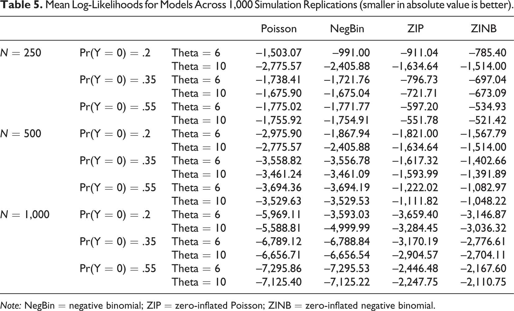
Note: NegBin = negative binomial; ZIP = zero-inflated Poisson; ZINB = zero-inflated negative binomial.

Finally, we compare the results of the simulation to the true parameter values; Tables 6 through 8 show the mean parameter estimates for sample sizes of 250, 500, and 1,000, respectively. Across all sample sizes, all models do a reasonable job of recovering the true parameter values for the six predictor variables, but only the zero-inflated models do a good job of recovering the correct value of the intercept—which is a clear advantage of the zero-inflated models versus even the negative binomial model, which seems to otherwise fit the data adequately when the percentage of zeros is low. Notably, even for the largest sample size, the estimates of the intercept continue to be quite poor for the Poisson, quasi-Poisson, and negative binomial model, even though they provide good estimates of the parameters.

Table 6.

Mean Parameter Estimates for Each Model Over 1,000 Simulation Replications for Sample Size = 250.

		Model	B0	X1	X2	X3	X4	X5	X6
	True value		2.680	.360	–.001	–.010	–.010	.080	–.080
Pr(Y = 0) = .2	Theta = 6	Poisson	2.448	.360	–.003	–.013	–.011	.083	–.081
		Quasi-Poisson	2.448	.360	–.003	–.013	–.011	.083	–.081
		NegBin	2.449	.359	–.004	–.013	–.010	.081	–.080
		ZIP	2.676	.360	–.001	–.011	–.010	.081	–.081
		ZINB	2.675	.361	–.001	–.012	–.010	.081	–.081
	Theta = 10	Poisson	2.454	.360	–.001	–.010	–.010	.079	–.080
		Quasi-Poisson	2.454	.360	–.001	–.010	–.010	.079	–.080
		NegBin	2.454	.360	–.001	–.010	–.010	.079	–.080
		ZIP	2.680	.360	–.002	–.009	–.010	.080	–.080
		ZINB	2.679	.361	–.001	–.010	–.010	.080	–.080
Pr(Y = 0) = .35	Theta = 6	Poisson	2.238	.360	–.001	–.010	–.012	.081	–.078
		Quasi-Poisson	2.238	.360	–.001	–.010	–.012	.081	–.078
		NegBin	2.238	.359	–.001	–.010	–.012	.082	–.078
		ZIP	2.677	.358	–.001	–.011	–.011	.078	–.080
		ZINB	2.676	.360	–.001	–.011	–.011	.079	–.080
	Theta = 10	Poisson	2.236	.360	–.001	–.011	–.007	.080	–.075
		Quasi-Poisson	2.236	.360	–.001	–.011	–.007	.080	–.075
		NegBin	2.236	.360	–.001	–.011	–.007	.080	–.075
		ZIP	2.677	.358	–.002	–.010	–.009	.078	–.078
		ZINB	2.677	.360	–.001	–.010	–.009	.079	–.079
Pr(Y = 0) = .55	Theta = 6	Poisson	1.851	.358	.001	–.015	–.009	.080	–.079
		Quasi-Poisson	1.851	.358	.001	–.015	–.009	.080	–.079
		NegBin	1.851	.358	.001	–.014	–.009	.080	–.079
		ZIP	2.673	.359	.001	–.011	–.009	.079	–.080
		ZINB	2.671	.361	.001	–.011	–.009	.080	–.080
	Theta = 10	Poisson	1.858	.360	–.001	–.012	–.008	.082	–.078
		Quasi-Poisson	1.858	.360	–.001	–.012	–.008	.082	–.078
		NegBin	1.858	.360	–.001	–.012	–.008	.082	–.078
		ZIP	2.676	.359	–.001	–.011	–.011	.081	–.078
		ZINB	2.675	.360	–.001	–.010	–.011	.081	–.078

Note: NegBin = negative binomial; ZIP = zero-inflated Poisson; ZINB = zero-inflated negative binomial.

Table 7.

Mean Parameter Estimates for Each Model Over 1,000 Simulation Replications for Sample Size = 500.

		Model	B0	X1	X2	X3	X4	X5	X6
	True value		2.680	.360	–.001	–.010	–.010	.080	–.080
Pr(Y = 0) = .2	Theta = 6	Poisson	2.451	.359	–.001	–.012	–.008	.080	–.080
		Quasi-Poisson	2.451	.359	–.001	–.012	–.008	.080	–.080
		NegBin	2.452	.359	–.001	–.012	–.009	.080	–.080
		ZIP	2.679	.359	–.001	–.011	–.009	.080	–.081
		ZINB	2.677	.360	–.001	–.011	–.010	.080	–.081
	Theta = 10	Poisson	2.454	.360	–.001	–.010	–.010	.079	–.080
		Quasi-Poisson	2.454	.360	–.001	–.010	–.010	.079	–.080
		NegBin	2.454	.360	–.001	–.010	–.010	.079	–.080
		ZIP	2.680	.360	–.002	–.009	–.010	.080	–.080
		ZINB	2.679	.361	–.001	–.010	–.010	.080	–.080
Pr(Y = 0) = .35	Theta = 6	Poisson	2.243	.360	.000	–.009	–.008	.081	–.083
		Quasi-Poisson	2.243	.360	.000	–.009	–.008	.081	–.083
		NegBin	2.243	.360	.000	–.009	–.008	.081	–.083
		ZIP	2.679	.359	–.001	–.010	–.009	.081	–.081
		ZINB	2.678	.360	–.001	–.010	–.010	.081	–.081
	Theta = 10	Poisson	2.241	.358	–.001	–.011	–.010	.084	–.080
		Quasi-Poisson	2.241	.358	–.001	–.011	–.010	.084	–.080
		NegBin	2.241	.358	–.001	–.011	–.010	.084	–.080
		ZIP	2.679	.358	–.001	–.011	–.010	.081	–.080
		ZINB	2.678	.359	–.001	–.011	–.010	.081	–.081
Pr(Y = 0) = .55	Theta = 6	Poisson	1.867	.356	.001	–.012	–.008	.081	–.079
		Quasi-Poisson	1.867	.356	.001	–.012	–.008	.081	–.079
		NegBin	1.867	.356	.001	–.012	–.008	.081	–.079
		ZIP	2.677	.358	–.001	–.011	–.011	.080	–.079
		ZINB	2.676	.360	–.001	–.011	–.011	.081	–.079
	Theta = 10	Poisson	1.867	.360	–.002	–.008	–.011	.080	–.083
		Quasi-Poisson	1.867	.360	–.002	–.008	–.011	.080	–.083
		NegBin	1.867	.360	–.002	–.008	–.011	.080	–.083
		ZIP	2.678	.358	–.002	–.010	–.011	.081	–.082
		ZINB	2.677	.358	–.002	–.010	–.011	.081	–.081

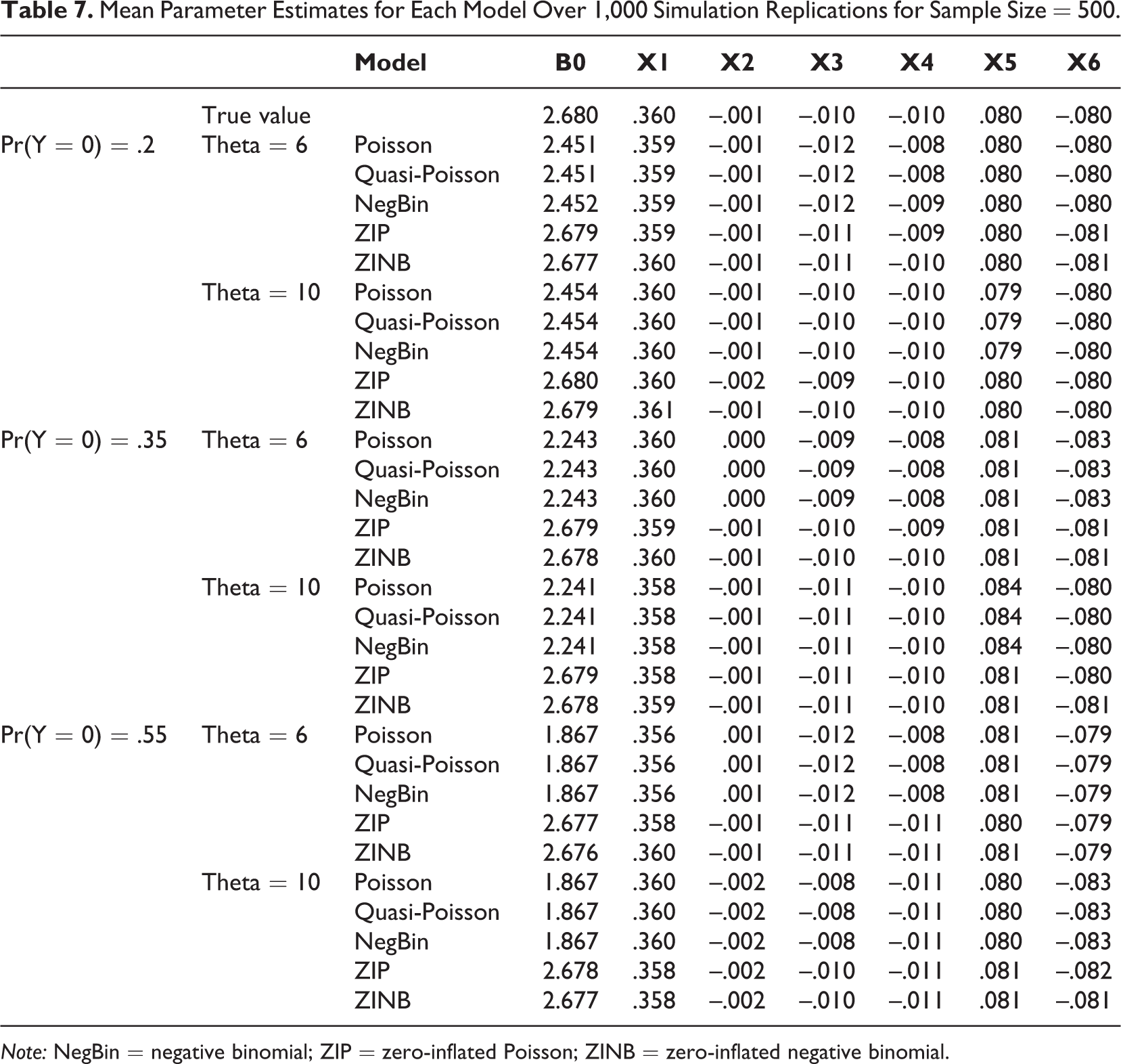
Note: NegBin = negative binomial; ZIP = zero-inflated Poisson; ZINB = zero-inflated negative binomial.

Table 8.

Mean Parameter Estimates for Each Model Over 1,000 Simulation Replications for Sample Size = 1,000.

		Model	B0	X1	X2	X3	X4	X5	X6
	True value		2.680	.360	–.001	–.010	–.010	.080	–.080
Pr(Y = 0) = .2	Theta = 6	Poisson	2.455	.359	–.001	–.008	–.009	.081	–.080
		Quasi-Poisson	2.455	.359	–.001	–.008	–.009	.081	–.080
		NegBin	2.455	.360	–.001	–.008	–.008	.082	–.080
		ZIP	2.680	.359	.000	–.008	–.009	.080	–.080
		ZINB	2.679	.360	.000	–.009	–.009	.081	–.080
	Theta = 10	Poisson	2.455	.360	.000	–.010	–.009	.079	–.079
		Quasi-Poisson	2.455	.360	.000	–.010	–.009	.079	–.079
		NegBin	2.455	.359	.000	–.010	–.009	.079	–.079
		ZIP	2.680	.360	–.001	–.010	–.009	.079	–.080
		ZINB	2.679	.360	–.001	–.010	–.009	.079	–.080
Pr(Y = 0) = .35	Theta = 6	Poisson	2.245	.360	–.002	–.010	–.012	.079	–.080
		Quasi-Poisson	2.245	.360	–.002	–.010	–.012	.079	–.080
		NegBin	2.245	.360	–.002	–.010	–.012	.079	–.080
		ZIP	2.680	.359	–.001	–.010	–.009	.080	–.080
		ZINB	2.679	.360	–.001	–.010	–.009	.080	–.080
		Poisson	2.245	.359	.001	–.011	–.010	.079	–.080
	Theta = 10	Quasi-Poisson	2.245	.359	.001	–.011	–.010	.079	–.080
		NegBin	2.245	.359	.001	–.011	–.010	.079	–.080
		ZIP	2.680	.360	–.001	–.010	–.010	.079	–.080
		ZINB	2.679	.360	–.001	–.010	–.010	.080	–.080
Pr(Y = 0) = .55	Theta = 6	Poisson	1.875	.360	–.001	–.010	–.009	.079	–.081
		Quasi-Poisson	1.875	.360	–.001	–.010	–.009	.079	–.081
		NegBin	1.875	.360	–.001	–.010	–.009	.079	–.081
		ZIP	2.679	.359	–.001	–.010	–.009	.079	–.079
		ZINB	2.677	.360	–.001	–.010	–.010	.079	–.080
	Theta = 10	Poisson	1.877	.357	–.001	–.008	–.010	.082	–.078
		Quasi-Poisson	1.877	.357	–.001	–.008	–.010	.082	–.078
		NegBin	1.877	.357	–.001	–.008	–.010	.082	–.078
		ZIP	2.678	.359	–.001	–.010	–.010	.081	–.080
		ZINB	2.678	.360	–.001	–.010	–.010	.081	–.080

Note: NegBin = negative binomial; ZIP = zero-inflated Poisson; ZINB = zero-inflated negative binomial.

A Concise Guideline

Figure 3 presents a simple decision tree for guiding the choice among the four types of models: Poisson, negative binomial, and their zero-inflated versions. We only focus on the two main factors presented in this article, namely, overdispersion and excess zeros—issues that management researchers frequently face when working on count-based dependent variables. As previously noted, most statistical software has not implemented the panel versions of the zero-inflated models. There are complex ways to specify these models, and so far zero-inflated panels have been shown to be a superior fit to more basic Poisson and negative binomial panel regressions (Boucher, Denuit, & Guillén, 2009). Accordingly, the recommendations generally hold for both panel and cross-sectional data; however, panel data with zero-inflated models is a much bigger challenge to implement in practice. Moreover, we do not deal with other more subtle and technical issues, such as whether it is important to estimate the probability distribution of an individual count (Gardner et al., 1995), nor do we go into detail whether fixed or random effects are more appropriate, since as previously noted, this is an area that is germane to each unique data set.

Figure 3.

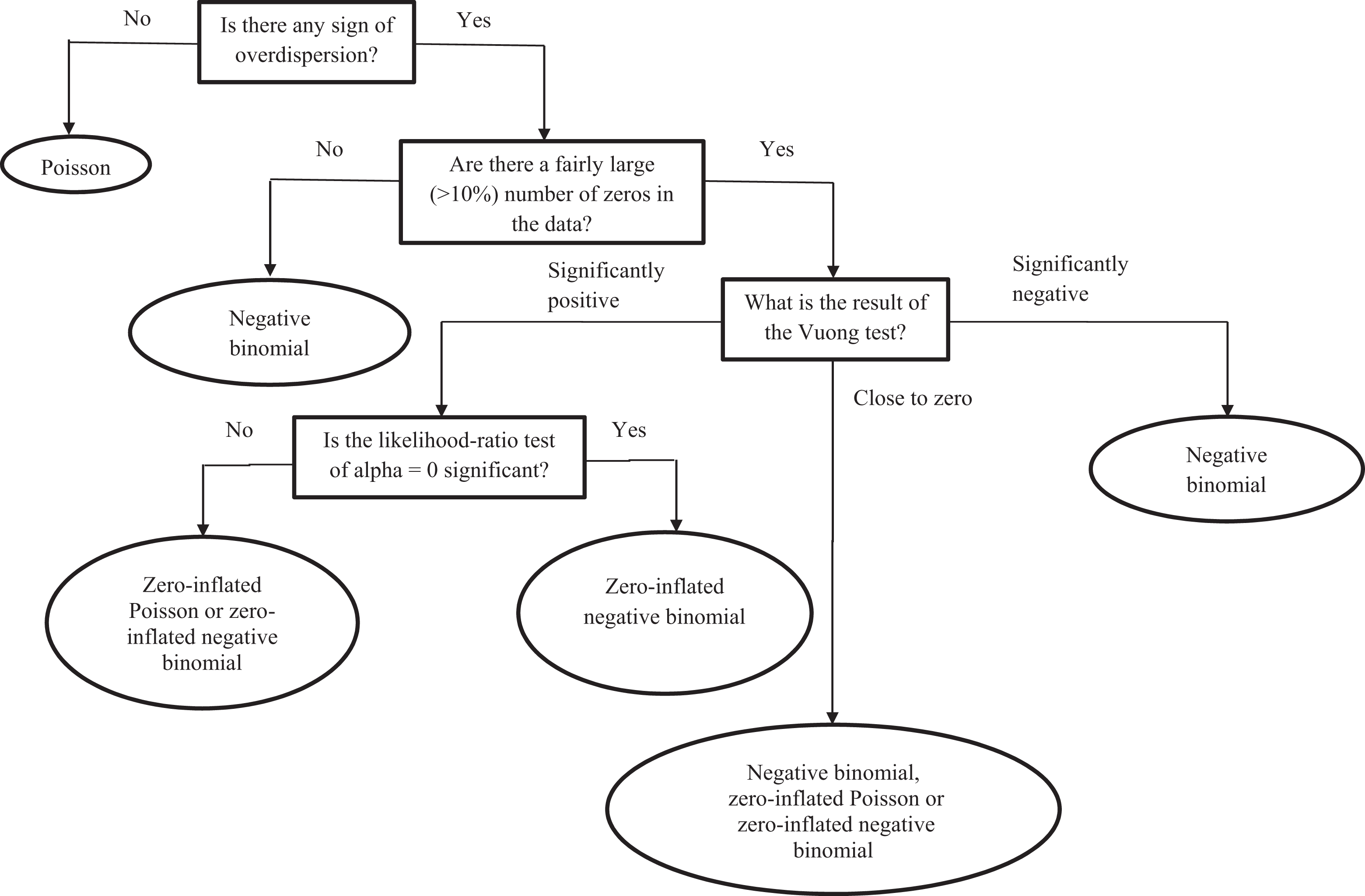
Decision tree with count-based dependent variables.

In line with most statistical textbooks (Cameron & Trivedi, 1998), unless the data display equidispersion, the negative binomial should be where most researchers begin their analysis. Only in compelling cases should the basic Poisson model be used, especially given that most statistical software such as STATA will default to the basic Poisson in the scenario of equidispersion. Therefore, given the simplicity of estimating the negative binomial, some comparison of the models should be implemented. The more complicated decision is where a researcher has to determine whether there is a presence of excess zeros in the data, which is probably the most common cause of overdispersion in management research. There is little guidance in the literature with respect to the threshold percentage of zeros above which the data set is considered having excess zeros. Based on our findings from the replication of Ornstein’s (1976) data, along with the simulation we adopt a conservative threshold of 10% of the observations taking the value of zero. When the count of zeros is below this level, the basic negative binomial may be appropriate, but a Vuong test can aid in such scenarios.

When the percentage of zeros exceeds 10% we recommend running the zero-inflated Poisson or zero-inflated negative binomial model together with the Vuong test, which compares a zero-inflated model with its corresponding basic version. The Vuong statistic has a standard normal distribution with significantly positive values favoring the zero-inflated model and with significantly negative values favoring the basic version (Long, 1997). A caveat here is that if the Vuong test is conducted on a zero-inflated Poisson model and a significantly negative statistic is generated, we recommend against using the basic Poisson model for the simple reason that the model is unsuitable for analyzing overdispersed data. The researcher should drop the zero-inflated Poisson model, try zero-inflated negative binomial, and rerun the Vuong test. If the Vuong statistic is still significantly negative, the basic negative binomial model should be adopted. If the Vuong statistic is significantly positive, the likelihood ratio test of alpha = 0 has to be conducted. A significant test result indicates that the zero-inflated negative binomial model should be adopted while an insignificant result indicates that either of the zero-inflated models is appropriate. Finally, if the absolute value of the Vuong statistic is close to zero, neither the zero-inflated nor the basic model is favored. In this case, the researcher may choose among the negative binomial and the two zero-inflated models. Ultimately, the final choice may depend on factors that are not discussed in this paper.

Conclusion

By illustrating with simulation and replicated data, we highlight some of the challenges that researchers face when deciding how to specify models when the outcome variable is a count-based measure. Our motivation for this paper stemmed from the disappointing discovery of having the results of a research project change from strongly significant under the basic Poisson estimation to no longer significant with a more appropriately specified negative binomial model. Originally, we used the Poisson model “following past literature” as many others do. We just so happened to pick one of the papers using the basic Poisson model as a starting point since it was widely cited. However, upon reviewing more papers we realized that our data displayed signs of overdispersion, and consequently, we also realized that our once significant results were no longer significant with the proper statistical estimation.

Admittedly frustrated by the results, we were interested to see if others might have made similar mistakes but nevertheless made it through the review process. To our surprise, we found that approximately one out of four of the papers that had count-based outcomes presented the basic Poisson regression only. Moreover, in most of those articles there was little discussion about whether or not alternative models were tested.

In sum, our goal is to provide a succinct and relatively simple overview of potential problems and solutions when analyzing data with count-based dependent variables. Our review highlights that there are opportunities to improve upon existing research. We show that there can be substantial changes in findings, depending on the type of count-based model that is specified. In general our simulation and replication show that the negative binomial model is often more appropriate than the basic Poisson model and should be the starting point for most count-based research (especially in cross-sectional data). When there are excess zeros in the data, zero-inflated Poisson and zero-inflated negative binomial models are also viable alternatives to basic Poisson—and in our examples, are both clearly a better fit. Moreover, we recommend that authors offer more transparency in the proportion of zeros comprising their data and the specification addressing the zeros, which would help readers judge whether the best model is being used.

Our paper underscores management researchers’ need to understand the challenges and limitations of their data (Ketchen, Boyd, & Bergh, 2008). This is important since surveys indicate that most management doctoral students are not well trained with count-based regression models such as Poisson or negative binomial (Shook et al., 2003). By providing a concise and simple guideline in count-based analysis we hope that management journals can continue leading the way in using the most rigorous and advanced methodology when compared to other disciplines.

Footnotes

Appendix

Declaration of Conflicting Interests

The author(s) declared no potential conflicts of interest with respect to the research, authorship, and/or publication of this article.

Funding

The author(s) received no financial support for the research, authorship, and/or publication of this article.

Notes

References

Allison

P. D.

Waterman

R. P.

(2002). Fixed-effects negative binomial regression models. Sociological Methodology, 32 (1), 247–265.

Antonakis

Bastardoz

Liu

Schriesheim

C. A.

(2014). What makes articles highly cited? Leadership Quarterly, 25 (1), 152–179.

Berdahl

J. L.

Moore

(2006). Workplace harassment: Double jeopardy for minority women. Journal of Applied Psychology, 91 (2), 426–436.

Bettis

R. A.

(2012). The search for asterisks: Compromised statistical tests and flawed theories. Strategic Management Journal, 33 (1), 108–113.

Boucher

J. P.

Denuit

Guillén

(2009). Number of accidents or number of claims? An approach with zero-inflated poisson models for panel data. Journal of Risk and Insurance, 76 (4), 821–846.

Cameron

A. C.

Trivedi

P. K.

(1998). Regression analysis of count data. New York, NY: Cambridge University Press.

Cardinal

L. B.

(2001). Technological innovation in the pharmaceutical industry: The use of organizational control in managing research and development. Organization Science, 12 (1), 19–36.

Chang

S. J.

Chung

C. N.

Mahmood

I. P.

(2006). When and how does business group affiliation promote firm innovation? A tale of two emerging economies. Organization Science, 17(5), 637–656.

Corredoira

R. A.

Rosenkopf

(2010). Should auld acquaintance be forgot? The reverse transfer of knowledge through mobility ties. Strategic Management Journal, 31 (2), 159–181.

10.

Drukker

D. M.

(2007). My raw data contain evidence of both overdispersion and “excess zeros.” Stata. Retrieved from http://www.stata.com/support/faqs/statistics/overdispersion-and-excess-zeros/

11.

Fox

Weisberg

(2009). An R companion to applied regression. Thousand Oaks, CA: Sage.

12.

Gardner

Mulvey

E. P.

Shaw

E. C.

(1995). Regression analyses of counts and rates: Poisson, overdispersed Poisson, and negative binomial models. Psychological Bulletin, 118 (3), 392–404.

13.

Gelman

Carlin

J. B.

Stern

H. S.

Dunson

D. B.

Vehtari

Rubin

D. B.

(2013). Bayesian data analysis (3rd ed.). New York, NY: CRC Press.

14.

Gelman

Hill

(2007). Data analysis using regression and multilevel/hierarchical models. New York, NY: Cambridge University Press.

15.

Greene

W. H.

(2008). Functional forms for the negative binomial model for count data. Economics Letters, 99 (3), 585–590.

16.

Greene

W. H.

(2003). Econometric analysis. Upper Saddle River, NJ: Prentice Hall.

17.

Haleblian

J. J.

McNamara

Kolev

Dykes

B. J.

(2012). Exploring firm characteristics that differentiate leaders from followers in industry merger waves: A competitive dynamics perspective. Strategic Management Journal, 33(9), 1037–1052.

18.

Hausman

J. A.

Hall

B. H.

Griliches

(1984). Econometric models for count data with an application to the patents-R&D relationship. Econometrica, 52(4), 909–938.

19.

Hess

A. M.

Rothaermel

F. T.

(2011). When are assets complementary? Star scientists, strategic alliances, and innovation in the pharmaceutical industry. Strategic Management Journal, 32 (8), 895–909.

20.

Hoetker

Agarwal

(2007). Death hurts, but it isn’t fatal: The postexit diffusion of knowledge created by innovative companies. Academy of Management Journal, 50 (2), 446–467.

21.

Kennedy

(2003). A guide to econometrics. Cambridge, MA: MIT Press.

22.

Ketchen

D. J.

Boyd

B. K.

Bergh

D. D.

(2008). Research methods in strategic management: Past accomplishments and future challenges. Organizational Research Methods, 11(4), 643–658.

23.

Lin

Z. J.

Peng

M. W.

Yang

Sun

S. L.

(2009). How do networks and learning drive M&As? An institutional comparison between China and the United States. Strategic Management Journal, 30(10), 1113–1132.

24.

Long

J. S.

(1997). Regression models for categorical and limited dependent variables. Thousand Oaks, CA: Sage.

25.

Miller

K. D.

Tsang

E. W. K.

(2011). Testing management theories: Critical realist philosophy and research methods. Strategic Management Journal, 32 (2), 139–158.

26.

Ohly

Sonnentag

Pluntke

(2006). Routinization, work characteristics and their relationships with creative and proactive behaviors. Journal of Organizational Behavior, 27 (3), 257–279.

27.

Ornstein

M. D.

(1976). The boards and executives of the largest Canadian corporations: Size, composition, and interlocks. Canadian Journal of Sociology, 1(4), 411–437.

28.

Park

S. H.

Chen

Gallagher

(2002). Firm resources as moderators of the relationship between market growth and strategic alliances in semiconductor start-ups. Academy of Management Journal, 45(3), 527–545.

29.

Pe’Er

Gottschalg

(2011). Red and blue: the relationship between the institutional context and the performance of leveraged buyout investments. Strategic Management Journal, 32(12), 1356–1367.

30.

Penner-Hahn

Shaver

J. M.

(2005). Does international research and development increase patent output? An analysis of Japanese pharmaceutical firms. Strategic Management Journal, 26 (2), 121–140.

31.

R Development Core Team. (2013). R: A language and environment for statistical computing. Vienna, Austria: R Foundation for Statistical Computing.

32.

Shook

C. L.

Ketchen

D. J.

Cycyota

C. S.

Crockett

(2003). Data analytic trends and training in strategic management. Strategic Management Journal, 24 (12), 1231–1237.

33.

Soh

P. H.

(2010). Network patterns and competitive advantage before the emergence of a dominant design. Strategic Management Journal, 31 (4), 438–461.

34.

C. A.

(2011). The advantage of foreignness in innovation. Strategic Management Journal, 32(11), 1232–1242.

35.

Vuong

Q. H.

(1989). Likelihood ratio tests for model selection and non-nested hypotheses. Econometrica, 57(2), 307–333.

36.

Wang

Liu

Zhan

Shi

(2010). Daily work-family conflict and alcohol use: Testing the cross-level moderation effects of peer drinking norms and social support. Journal of Applied Psychology, 95 (2), 377–386.

37.

Zeileis

Kleiber

Jackman

(2008). Regression models for count data in R. Journal of Statistical Software, 27 (8). URL: http://www.jstatsoft.org/v27/i08/