Condition 9 and 10 Tests of Model Confirmation: A Review of James,Mulaik,and Brett (1982) and Contemporary Alternatives

Abstract

Structural equation modeling (SEM) serves as one of the most important advances in the social sciences in the past 40 years. Through a combination of factor analysis and path analysis, SEM allows organizational researchers to test causal models while accounting for random and nonrandom (bias) measurement error. SEM is now one of the most commonly used analytic techniques and its modern day ubiquity can be traced in large part to a series of intellectual contributions by Larry James. The current article focuses on the seminal work, James, Mulaik, and Brett (1982), and the unique contribution of the “conditions” required for appropriate confirmatory inference with the path and latent variable models. We discuss the importance of James et al.’s Condition 9 and 10 tests, systematically review 14 years of studies using SEM in leading management journals and reanalyze results based on new techniques that extend James et al. (1982), and conclude with suggestions for improved Condition 9 and 10 assessments.

Keywords

structural equation modeling measurement models factor analysis quantitative research

The social sciences, including the disciplines of industrial/organizational psychology and management, were greatly impacted by the emergence of multiple linear regression in the late 1960s. Seminal articles by Cohen (1968) and Darlington (1968) provided introductions to the technique, examples of its use, and discussion of key issues to be considered by those wanting to apply it to their substantive research problems. The subsequent use of multiple regression by organizational researchers in the 1970s has been documented by Austin (2002). Around the same time, an influential article by Werts and Linn (1970) was among the first to describe the use of multiple linear regression for testing “causal models,” with this approach being referred to as path analysis. Within this context, organizational researchers increasingly adopted path analysis, and key review articles by Feldman (1975) and Billings and Wroten (1978) documented its use. Feldman described its emergence as an analytical technique, noting it represented progress, in that it allowed “development and testing of explicit causal propositions under conditions maximizing external validity” (p. 663).

The testing of causal models by organizational researchers took a big step forward in the early 1980s as advancements involving latent variables occurred. Latent variable models are often described conceptually as a combination of factor analysis and linear regression models, although ordinary least squares (OLS) techniques are not directly involved. Among its several strengths, the use of latent variables allowed for overcoming a key limitation of the use of regression for testing such models, in that the effects of random (and nonrandom) measurement error could be accommodated. Organizational scholars wanting to use latent variables were greatly influenced by several books at this time, including Duncan (1975), Kenny (1979), Jöreskog and Sörbom (1979), and Bagozzi (1980). However, no source impacted their/our field and its approach to causal modeling as much as the seminal book by James, Mulaik, and Brett (1982). Although all these different sources covered many of the same statistical and technical issues, a unique contribution of James et al. was their presentation of the “conditions” required for appropriate confirmatory inference with the path and latent variable models. They claimed, “There is a serious need to specify the conditions that justify the application of confirmatory analysis and the use of the results of the confirmatory analysis to support causal inference” (p. 2). Some of these conditions related to the role of theory, assumptions related to causal order and direction of variable relations, self-containment, boundary conditions, the stability of the model, and operationalization of the variables. However, we feel that their discussion of Condition 9 and Condition 10 tests may have had the greatest impact on organizational researchers. The former test relates to an empirical support for the equations of the model, while the latter describes the fit between the structural model and empirical data.

The fields of management and industrial/organizational psychology have evolved since the 1980s to the point where structural equation and confirmatory modeling is one of the most widely used analytical approaches with observational designs. Over the years, several authors provided reviews of studies using the technique, including James and James (1989), Harris and Schaubroeck (1990), Medsker, Williams, and Holahan (1994), Shook, Ketchen, Hult, and Kacmar (2004), and Williams, Gavin, and Hartman (2004). These reviews included discussion of research practices from empirical examples in the micro- and macro-organizational literature. However, since the early 1990s there has been no review of organizational research using latent variable techniques that focus on model confirmation issues, in spite of the frequency of their use (which we will document). At the same time, there has been a continued development of new techniques related to Conditions 9 and 10 of James et al. (1982).

As a result, in this article we honor and extend the contributions of Lawrence R. James to organizational research based on structural equation methods in four key ways. First, we will review the James et al. (1982) presentation of Condition 9 and 10 tests, so as to provide the background needed to understand our second contribution, a review of recent substantive research using SEM, and approaches taken in these articles to model confirmation. In this review we will document different techniques and indices used to see if Conditions 9 and 10 have been met, as well as relations among these different approaches. In the third section of our article we will provide a reanalysis of results from 116 empirical studies of management that used structural equation models with latent variables. This reanalysis will occur using a combination of approaches to model confirmation based on new techniques that extend James et al. (1982). We will see if original conclusions about models are upheld with the use of new approaches. Finally, in our final section we provide suggestions for improved Condition 9 and 10 assessment and a briefly introduce organizational researchers to other issues related to model evaluation being investigated currently by quantitative methodologists.

A Historical Perspective on Condition 9 and 10 Tests

James et al. (1982) initially discuss these two tests in the context of path analysis models using manifest variables (ignoring measurement error). For our presentation, it is assumed that these models include paths that are contained in the model, and that there are other potential paths that are omitted, which is to say are not in the model. It is further assumed that decisions about whether paths are specified as being in or out of the model are guided by theory. As an example, a full mediated model proposing that an exogenous variable (X) influences a mediator (M) that then influences an outcome (Y) would include an indirect effects in the mediation model and associated paths. A path representing the direct effect of the exogenous variable on the outcomes variable would not be included (due to the hypothesized full mediation). An example of such a model is presented in Figure 1a, along with a summary of how Condition 9 and 10 requirements can be met based on James et al. (1982). In describing Condition 9 tests for a model, James et al. note they focus on testing whether certain causal parameters are different from zero. Specifically, parameters that are included because they represent paths describing relations among variables that are predicted based on theory (e.g., b₁ ≠ 0, b₂ ≠ 0). Initially they state, “If the estimate of a structural parameter is significantly different from zero, then the prediction is regarded as confirmed” (p. 61), and they elaborate that “since causal relations are indicated by non-zero structural parameters in structural equations,” empirical support is provided by “statistical tests that reveal the corresponding estimates of free structural parameters differ significantly from zero” (p. 140). Within the context of models with manifest variables, James et al. (1982) summarize arguments for how if key assumptions are met, multiple linear regression and resulting OLS estimates and their significance can be used for Condition 9 tests.

Figure 1.

(a) Example path analysis model (full mediation), proposes b₁ ≠ 0, b₂ ≠ 0, b₃ = 0. Condition 9: Requires b₁ ≠ 0 and b₂ ≠ 0. 1) Met if b₁ and b₂ confidence intervals do not include 0. Condition 10: Requires b₃ = 0. 1) Met if b₃ confidence interval includes 0 (omitted parameter test). Let r*_xy = reproduced correlation = b₁ x b_2. 2) Met if r_xy – r*_xy = 0 (reproduced correlation test). (b) Example latent variable model (full mediation). Proposes γ₁ ≠ 0, β₁ ≠ 0, γ₂ = 0. Condition 9: Requires γ₁ ≠ 0 and β₁ ≠ 0. 1) Met if γ₁ and β₁ confidence intervals do not include 0. Let M_T-2 constrain γ₁ and β₁ = 0. 2) Met if χ² _T-2 – χ² _T significant. Condition 10: Requires γ₂ = 0. Let M_T+1 include γ₂ ≠ 0. (1) Met if γ₂ confidence interval includes 0. (2) Met if χ² _T – χ² _T+1 not significant. (3) Met if M_T goodness of fit is adequate.

In beginning their discussion of Condition 10 tests for path analysis models using manifest variables, James et al. (p. 81) emphasize that “it is quite possible for all of the estimated parameters to be significantly different from zero when the structural model is invalid.” As a result, of key priority in the model evaluation process is the examination of evidence that the model has validity, which is to say it is correctly or nearly correctly specified. Otherwise, all conclusions reached about Condition 9 fulfillment based on parameters’ significance tests are not valid. We emphasize our belief based on experience that many organizational researchers do not fully understand this key point as they interpret results of their analyses. Their Condition 10 tests evaluate the degree to which such correct specification has occurred, and James et al. discuss two approaches to the Condition 10 test. The first is referred to as the omitted parameter test, and when used to assess a model that has paths left out based on theory (e.g., b₃ = 0), it is implemented by examining an alternative model that actually includes the paths omitted from the original model. This test of omitted paths is implemented by adding the variables associated with the predictors that are proposed as being nonsignificant to the equations for their respective dependent variables. Given that the paths left out imply the prediction that they are not different from zero, Condition 10 support is obtained when the estimated paths from these added predictors in the alternative model are NOT statistically different from zero.

The second approach for the same purpose, which they describe as more subtle, is referred to as the reproduced correlation test. In introducing this test, they note, “The key to the reproduced correlation test is to decompose correlations among variables in a structural model into functions of path coefficients and, if necessary, unanalyzed correlations among exogenous variables” (p. 83). They further describe that once this is done, the path coefficient estimates can be used to compute “reproduced” correlations (e.g., r*_xy = b₁ x b₂) among the model variables based on the model specification, which can be compared to the actual sample correlations (e.g., r_xy) used to obtain the estimates. In summarizing, they state, “Divergence of reproduced from observed correlations disconfirms predictions regarding the reproduced correlations and implies that a-priori hypotheses are incorrect. Reproduced correlations equal to the observed correlations denote confirmation of predictions an imply that the a priori hypotheses may be valid” (p. 89). In our example this is indicated if r_xy – r*_xy = 0.

In discussing Condition 9 and 10 tests for latent variable models, James et al. note that for these models full information estimation (e.g., maximum likelihood) would likely be used (rather than OLS regression) and would provide for three kinds of statistical tests for assessing Conditions 9 and 10 (e.g., James et al., p. 141). An example of a latent variable model with multiple indicators corresponding to the path analysis model is presented in Figure 1b, along with a summary of how Condition 9 and 10 requirements can be met. First, since standard errors of parameter estimates are obtained this allows confidence interval tests of the individual free parameters. They add that the relevant standard errors are conditional, which is to say are based on the fixed and constrained parameters of the model. As they elaborate, these tests are only unbiased if the model has been demonstrated to have good fit with the data, and if many tests are conducted a concern about rising Type I error rates is warranted. Second, tests are available for comparing two nested models, where nesting typically means the two models being compared are identical except one includes some type of constraint(s) on parameters that are estimated in the other (such as a path or multiple paths set to zero). Finally, there are tests of the overall goodness of fit of the model, reflecting the difference between the sample covariance matrix used to obtain the estimates, and a predicted covariance matrix based on the final parameter estimates from any given theoretical model. We note the conceptual similarity between this approach and the reproduced correlation test described for manifest variable models.

For Condition 9 tests of whether certain causal parameters are different from zero, James et al. describe how with latent variable models confidence intervals around estimates (in our case γ₁ and β₁) are examined, similar to what occurs with OLS estimates. If such an interval does not include zero, the conclusion is that the parameter differs significantly from zero, “thereby indicating a causal connection between the variables.” After describing how a chi-square statistic for a model is obtained, they also describe how chi-square difference tests can be used to compare nested models that differ such that one or more paths are excluded, as an alternative or supplement to the confidence interval tests. They elaborate, “If the difference in chi-squares between two models is significant, one rejects the null hypothesis about the fixed parameter(s). Such a result provides support for the path(s) associated with the parameter(s), and their causal proposition(s)” (p. 141). In our example let M_T include γ₁ and β₁ and M_T-2 sets these two paths to zero: Condition 9 is met if χ² _T-2 – χ² _T is significant.

For Condition 10 tests with latent variable models, James et al. describe two kinds of approaches. First, they extend the omitted parameter test logic to latent variable models and suggest comparing models that include proposed paths with models that also include paths that are predicted to be zero (e.g., γ₂). Support for Condition 10 is obtained if the resulting chi-square difference is NOT statistically significant, since this leads to the conclusion that the proposal to exclude these paths is supported. In our example let M_T+1 include all three paths, then Condition 10 is met if χ² _T – χ² _T+1 is NOT significant. For the second type of approach, it is based on the recognition that with large sample sizes, statistical power will be high, and as a result even minute differences between two models will be detected. As a result they recommended the use of the normed fit index (NFI; Bentler & Bonett, 1980): “This index gives the relative decrease in the lack of fit between two nested models, one less restricted than the other” (p. 135). As for its use, they state it “provides a nonstatistical assessment of the adequacy of a model’s fit to data, which may be used to determine whether, on practical grounds, a model may be of value in describing a particular set of data” (p. 155). In addition to the NFI, James et al. recommended the efficiency index of Khattab and Hocevar (1982), which they describe as representing “the per parameter ‘or degree of freedom’ average increase in fit” (p. 155). Thus in our example Condition 10 can also be met if M_T goodness of fit is adequate, as judged using guideline values.

To illustrate their recommendations, James et al. (1982) provided an integrative example with simulated data of model comparisons and goodness of fit measures that illustrated a nested sequence of model comparisons for use in Condition 9 and 10 tests. With their example, the sequence begins with a model in which all latent variables are linked to each other and all indicators (a just identified model, with zero chi-square and zero degrees of freedom). This model is compared to the next model that constrains to zero all the factor loadings linking latent variables to indicators other than their own. This model, which has come to be referred to as the saturated structural model and is statistically equivalent to a confirmatory factor analysis measurement model in which all latent variables are correlated with each other, is then compared to the theoretical path model, which includes restrictions on paths linking latent variables predicted to be zero based on theory. The researcher’s hope in this comparison is for a nonsignificant chi-square difference, indicating support for the excluding the paths predicted to be zero in the theoretical path model. This result provides confirmation for the exclusion of the omitted paths. Given this result, the theoretical path model is next compared to a model that proposes that all latent variables are unrelated, with the researcher’s goal being a significant chi-square difference test that indicates rejection of the restrictions of the paths and is a finding supportive of the theoretical model. With their example they also used significance of parameter estimates and the NFI and efficiency index to further evaluate the differences between the models.

Since the introduction of Condition 9 and 10 tests by James et al., others have followed their lead and many developments have occurred. For path analysis models, testing approaches have been further discussed, including Lance (1986) and LeBreton, Wu, and Bing (2008). For latent variable models, over the years a number of goodness-of-fit measures have been developed as extensions of the NFI and efficiency index (for general reviews, see Marsh, Balla, & McDonald, 1988; Medsker et al., 1994; West, Taylor, & Wu, 2012). As these measures were developed, they were evaluated both analytically and through simulation analysis. At this point, there are three main measures as revisions of those discussed by James et al. (1982) that are currently highly recommended. The CFI (comparative fit index; Bentler, 1990) is logically and computationally comparable to the NFI, but avoids problems of sample size bias. The RMSEA (root mean square error of approximation; Steiger & Lind, 1980) is somewhat similar to the efficiency index in that it takes into account the number of parameters estimated in the model, but has the advantage that a confidence interval is available to supplement the point estimate. And the standardized root mean square residual (e.g., Bentler, 1995) is based on the reproduced correlation test, as described by James et al. (1982). We note here that these indices are often called “global” fit indices because they summarize information on the entire latent variable model, including its links between the latent variables and the indicators, correlations between exogenous latent variables, and “structural” parameters representing causal relations among exogenous and endogenous latent variables. We will describe suggested guidelines for these three indices when we document the frequency of their use.

Condition 9 and 10 Tests in Practice: A Review From 2001 to 2014

The preceding review made the case that the foundation of contemporary approaches to model evaluation for organizational and social science researchers was established by James et al. (1982). But as is true in all areas of research methods and data analysis, there has been an evolution in model testing techniques, as old ones have been evaluated and new ones developed. The integration of new methods techniques into substantive research applications can be a slow process. In this process, reviews and evaluations of recently developed practices used by substantive researchers can lead to more complete information about how well they are implemented, whether they work as intended, and alternatives that might be better for future research. As such, in this section we build on past reviews by looking at studies from a more recent period not previously examined, as we document approaches organizational researchers have used to test for the fulfillment of Conditions 9 and 10. In the process we will generate new information about how often and why different approaches to testing these conditions lead to similar or different conclusions about models. This will be achieved by focusing on the three recommended approaches (CFI, RMSEA, SRMR) and the similarities of conclusions reached with their use. We will also document the use of other indices.

Method

Search Parameters and Inclusion Criteria

The present review spans all models tested with SEM between 2001 and 2014 in the Academy of Management Journal, Journal of Applied Psychology, Personnel Psychology, Journal of Management, Organizational Behavior and Human Decision Processes, and Strategic Management Journal. The decision to include these six journals was based on journal impact factors and prior reviews of the literature on this topic (i.e., James & James, 1989; Medsker et al., 1994). The most recent review, Medsker et al. (1994), used all of the above journals except for Journal of Management and Strategic Management Journal, which we included to increase the comprehensiveness of our review.

A variety of search terms and databases helped to identify all possible articles relevant to our review. The search identified articles between the specified dates that were published in the above-mentioned journals. These search terms included complete and truncated forms of the following words and acronyms common to SEM: structural, model, confirmatory, exploratory, parameter, Chi-square, SEM, CFI, NFI, RMSEA, GFI, RMSR, LISREL, Joreskög, Sorbom, EQS, Mplus, and AMOS. The databases used for searching were PsycINFO, the Academy of Management online retrieval system, ABI Inform, and Google Scholar.

We included only primary studies that incorporated structural models where paths between latent variables existed at a single level of analysis and latent variables were measured with multiple indicators. Put differently, we first excluded studies using meta analytic structural equation modeling technique. In addition, confirmatory and exploratory factor analyses, hierarchical linear modeling, multilevel SEM, single indicator latent variable models, and path models using multiple regression and partial least squares were all excluded based on this criterion. Also excluded were instances where the methodology was unclear or inconsistent. Finally, we excluded studies using multilevel confirmatory factor analysis and multilevel structural equation modeling as there is still controversy related to the appropriateness of applying standard fit indices to these advanced techniques (Ryu, 2014). The search yielded over 600 articles. Of these, 237 met the inclusion criteria. In multistudy articles, each study was examined separately and was included and coded individually if it met inclusion criteria. The final tally of included studies was 311. All articles as well as the coding sheet are available from the second author by request.

Coding Strategy

For each included study, we coded sample size, the level of analysis (i.e., individual, team, or firm), chi-square statistic (χ²) and the degrees of freedom for both the CFA measurement (saturated structural) model if available and for the theoretical path or structural model, and the values of the previously mentioned fit indices: CFI, RMSEA, and SRMR. For historical comparison, we also documented use of goodness of fit index (GFI; Tanaka & Huba, 1984), adjusted goodness of fit index (AGFI; Anderson & Gerbing, 1984), normed fit index (NFI; Bentler & Bonett, 1980), Tucker-Lewis index (TLI/NNFI; Tucker & Lewis, 1973), incremental fit index (IFI; Bollen, 1990), and parsimony normed fit index (PNFI; James et al., 1982). We summarize information on these indices and other model diagnostics in the appendix but will not discuss them further due to space constraints and because they have been largely discredited or superseded by more current tools and because they have been used much less frequently than the methods we will focus on.

Results

Table 1 presents a summary of information related to model fit and evaluation of the studies included in our review. It is organized around a whether a particular test or measure yields information about Condition 9 or Condition 10. We have noted previously that there are two main Condition 9 tests for latent variables. The first uses the standard errors of individual parameter estimates to test for statistical significance, either through a confidence interval or a direct null hypothesis statistical test (t test). As shown in Table 1, this test was almost universally used, with 98% of the studies using this approach. The second approach involves a nested model comparison using a chi-square difference test. The null hypothesis of this test is that the path(s) that are constrained to zero in the more restricted model are statistically different from zero, with a significant chi-square difference leading to a rejection of the null hypothesis. As shown in Table 1, this approach was also widely used—in 197 of the 311 samples (63%) a chi-square nested model comparison was conducted.

Table 1.

Use of Condition 9 and 10 tests from studies reviewed.

	Guidelines	k	%	M (SD)
Condition 9 Tests
t test parameters	p < .05	304	98	—
Nested model comparison	Δχ²; p > .10	197	63	—
Condition 10 Tests
χ²	p > .10	287	92	594.73 (1066.85)
CFI	>.95	280	90	0.95 (0.03)
RMSEA	<.08	243	78	0.06 (0.02)
RMSEA CI	<.05, <.10	29	9	—
SRMR	<.10	133	43	0.06 (0.02)

Note: k = number of studies; SD = standard deviation; CFI = comparative fit index; RMSEA = root mean square error of approximation; CI = confidence interval; SRMR = standardized root mean square residual.

The results related to Condition 10 tests are also shown in Table 1, with additional information presented in Figure 1. As shown in Table 1, the chi-square statistic and its probability level is nearly always reported, but seldom used to make judgments about the model because it is a test that the model is perfect (which is seen as unrealistic) and because it is influenced by sample size and violations of normality (e.g., Kline, 2015). Instead of simply using the chi-square result, researchers focus on measures of approximate fit. The CFI is a goodness of fit index, with higher values indicating a better model. The CFI was used in 280 of the 311 (90%) studies in our review. The mean value of CFI was .95, which according to the often cited guideline of .95 (Kline, 2015), this indicates good model fit. As shown in Figure 2, we found a high prevalence of CFI values just above the .90 and .95 thresholds, and a low prevalence of CFI values just under the thresholds. For example, .929 and .949, there were 41 studies, but between .950 and .970, there were 111 studies.

Figure 2.

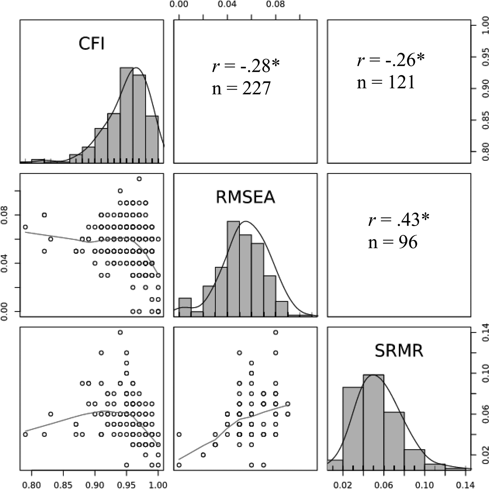
Frequency distributions, scatterplots, and correlations among CFI, RMSEA, SRMR.

The RMSEA is a badness of fit index, with higher values indicating a worse fitting model, and it was reported in 243 (78%) studies (see Table 1). The mean RMSEA was 0.06 indicating good fit relative to an often cited guideline (RMSEA ≤ .08). As with the CFI the number of studies that barely met thresholds far outpaced those that barely did not. For example, there were 82 studies with RMSEA values between .060 and .079 and 21 RMSEA values exactly at .080. That is, there were 103 studies with RMSEAs that exactly or barely met the traditional .080 threshold. Conversely, there were only 13 with values of .081 or higher (see Figure 2). More recent work with the RMSEA has pointed to the need to supplement the examination of a RMSEA point-estimate by examining its confidence interval (e.g., Kline, 2015). It is commonly recommended (e.g., Chen, Curran, Bollen, Kirby, & Paxton, 2008) that the point-estimate of the RMSEA be used in conjunction with its 90% confidence interval, such that a path model would be rejected if the lower bound of the confidence interval was greater than .05 or if the upper bound was greater than .10 (regardless of its point-estimate value). The use of this confidence interval “reflects the degree of uncertainty associated with the RMSEA as a point-estimate,” and “acknowledges that the RMSEA (and all other model fit indexes) are sample statistics subject to sampling error” (Kline, 2015, p. 139). As shown in Table 1, only 29 (9%) studies reported the RMSEA confidence interval.

Finally, the third fit index we will discuss is more directly linked to the residual covariance matrix (∑_res), and it is also a badness of fit index with larger values indicating worse fit. The SRMR (standardized root mean square residual) is obtained by taking the square root of the average of the squared values of ∑_res, after the residuals have been transformed to a correlation metric. As such, the SRMR provides a summary of the entire matrix of residuals in a correlation metric for a given model. Kline (2015) has suggested a .10 target guideline value. As shown in Table 1, the SRMR was used in 133 (43%) studies, and the mean SRMR in our sample is .06. Again, results in Figure 2 indicate that values at or near the threshold of .10 were far more frequent than those just falling above it with 20 studies reporting SRMR values between .08 and .10 and only 4 studies reporting SRMR above .10.

Use of Multiple Fit Measures

Given the results presented in Table 1, it should not be surprising that many studies used more than one approach to Condition 9 and 10 tests, especially given that all commonly used statistical software report results for multiple indices. We now focus on results from studies that used some combination of CFI, RMSEA, and SRMR for testing Condition 10, and place an emphasis on correspondence or agreement in decisions reached about models based on the use of multiple measures of fit within the same study. We look at three sets of information to try and understand the degree to which use of the three measures leads to similar conclusions about the models from the studies we reviewed. First, we focus on the correlations among the three primary fit measures. The distributions, bivariate scatter plots, and correlations between the CFI, RMSEA, and SRMR are also presented in Figure 2. The data are approximately normal and all three indices are correlated with one another at statistically significant levels. However, the magnitudes of these correlations fall somewhat short of what might be expected given the implicit assumption that model fit is unidimensional and different fit measures are highly correlated. Whereas simulation research (e.g., Hu & Bentler, 1998; Lai & Green, 2016; Marsh et al., 1988) tends to show these global fit measures to be highly correlated (|r| > .90), it would appear that in the studies we reviewed these indices are, at best, moderately correlated (.26 < |r| < .43). The correlation between the RMSEA and SRMR had the highest of the three values (.43), and both were correlated less with the CFI (–.28, –.26).

To further explore the issue of convergence between the three primary indices, we took a second approach. Table 2 presents a summary of the conclusions using commonly recommended thresholds of CFI > .95, RMSEA < .08, and SRMR < .10. There were 301 (97%) studies that reported one or more of these indices. Of these 301 studies, 35 reported only one index—results for these are reported in the first three rows of Table 2. As can be seen, when only one index was reported, the fit was usually deemed adequate. Of the 21 studies that reported the CFI, but not the RMSEA or SRMR, 13 met the threshold value of .95. For the 14 studies that reported either the RMSEA (k = 9) or SRMR (k = 5), all had acceptable fit. The more relevant information to fit index convergence is shown in the last four rows of Table 2. When just the CFI and RMSEA were reported, there tended to be convergence (86 out of 138 met both thresholds and 3 of the 138 met neither threshold, combined 64% agreement). However, there were a substantial number of studies where only the CFI threshold was met, but the RMSEA was not or vice versa (k = 43 + 6 = 49). When just the CFI and SRMR were reported, there was agreement in 24 of the 32 studies (21 with good fit, 3 agreeing on poor fit, combined agreement 75% agreement); while with the RMSEA and SRMR there was agreement in all 7 cases (and there were no cases where both indicated poor fit). When all three indices were reported (k = 89), there was again convergence among all three for meeting thresholds the majority of the time (49 out of 89, 55%), but a substantial amount of disagreement (only one or two indices of the three indicating good fit; k = 40 out of 89. So, in combination, when more than one global fit index was used (k = 266), there was agreement in 169 cases (163 indicating good fit, 6 indicating poor fit), for an overall rate of 64%.

Table 2.

Agreement Among Decisions Using CFI, RMSEA, and SRMR.

Indices Reported	k	Did Not Meet Threshold(s)	Met CFI Threshold Only	Met RMSEA Threshold Only	Met SRMR Threshold Only	Only Met CFI and RMSEA Thresholds	Only Met CFI and SRMR Thresholds	Only Met RMSEA and SRMR thresholds	Met All 3 Indices’ Thresholds
1. CFI only	21	8	13	—	—	—	—	—	—
2. RMSEA only	9	0	—	9	—	—	—	—	—
3. SRMR only	5	0	—	—	5	—	—	—	—
4. CFI and RMSEA	138	3	6	43	—	86	—	—	—
5. CFI and SRMR	32	3	1	—	7	—	21	—	—
6. RMSEA and SRMR	7	0	—	0	0	—	—	7	—
7. CFI, RMSEA, and SRMR	89	0	0	5	0	5	4	26	49

Note: k = number of studies; CFI = comparative fit index; RMSEA = root mean square error of approximation; SRMR = standardized root mean square residual. Bolded values indicate instances where all reported global fit indices suggested adequate fit.

Finally, our third approach to assessing correspondence between fit measures is based on Lai and Green (2016). They developed an index they named delta that assesses differential interpretation of RMSEA and CFI named delta, which is calculated as delta = RMSEA – (1 – CFI). As such delta values close to zero indicate a similar interpretation of a model using the two popular fit measures, while a positive delta indicates a more favorable value for CFI and a negative delta indicates a more favorable value for RMSEA. Results of our delta calculations for our 227 samples that included both fit measures can be found in Figure 3. Delta values had a mean of .006 and standard deviation of .035. Put differently, the RMSEA of models showed worse fit than the CFI. In terms directionality, 136 (59.9%) were positive, 23 (10.1%) yielded zero estimates, and 69 (30.0%) had negative values. In sum, the majority of deltas (122 or 53.7%) fell within the range of –.02 to .02, indicating fairly good agreement among values for the CFI and RMSEA.

Figure 3.

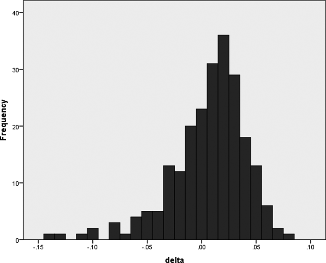
Frequency distribution of delta values from studies using CFI and RMSEA.

New Measures of Path Model Fit and Condition 9 and 10 Tests: A Reanalysis of Selected Studies

The preceding discussion of model fit focused on the complete latent variable multiple indicator model. One important trend over the past 15 years has been to acknowledge that such a model consists of multiple components, including (a) a part that includes links between the latent variables and their indicators, (b) a part representing correlations among exogenous latent variables, and (c) a part including what have been referred to as structural parameters shown graphically with single headed arrows that are in intended to represent causal relations among the latent variables. We will refer to this latter component as the “path” components, and note that arguments have been made that this component is what researchers are most interested in as they test theories of substantive relations (McDonald & Ho, 2002; O’Boyle & Williams, 2011). Given the importance of this path component, it should not be surprising that those concerned with model evaluation have raised the prospect that using fit measures that focus on the entire composite model to assess that path component of special interest may not be the optimal approach. Such a practice might result in the wrong conclusion being reached about what the substantive researcher is most interested in, the alignment of data to theory. For example, problems with components (a) and (b) described above might lower the overall measure of composite fit and obscure the fact that the path component is good. Perhaps a bigger problem is the possibility that a model with properly specified components (a) and (b) may yield values on global fit measures of the overall composite model that meet standards, at the same time that the model includes key misspecifications in the path component.

This concern has been investigated using fit measures that focus on the path component, as a supplement to traditional global fit measures that assess the entire composite model. The logic of these fit measures can be traced to Sobel and Bohrnstedt (1985), Mulaik et al. (1989), and Williams and Holahan (1994). Williams and O’Boyle (2011) used the label NSCI-P with an index originally presented by Williams and Holahan (1994). The NSCI-P follows the logic of the CFI, which judges a given model relative to the total amount of fit available fit as assessed by the difference in fit (χ²) between a worst possible model (Absolute Null) and a best possible model (Completely Saturated). We add the logic of the CFI follows that implied with a regression model, where the R² for a given model is judged relative to a range defined by the worst possible model (R² = 0) and the best possible model (R² = 1). In contrast, the NSCI-P judges the theoretical composite latent variable relative to a range of possible fit defined by the difference in χ² values between the worst possible path model (Structural Null) and the best possible path model (Saturated Structural, which is also equal to the CFA or Measurement Model associated with all latent variables). As a result, the NSCI-P is more sensitive in distinguishing between competing theoretical models for the same data. The algebraic basis of the NSCI-P and supporting simulation results have been presented by Williams and O’Boyle (2011).

Williams and O’Boyle (2011) also presented a second fit measure that focuses on the path model, using the label RMSEA-P to describe an alternative version of the RMSEA originally introduced by McDonald and Ho (2002). This index is computationally similar to the RMSEA, only replaces the χ² and df of the theoretical model with the χ² difference between the theoretical model and a simple CFA model (referred to as the measurement model) and the df difference between these same two models. Williams and O’Boyle reported simulation results indicating the RMSEA-P worked well with models with more than two indicators per latent variable. One reason is that it correctly identified models with only one path left out as misspecified and all true models had values that would have led them to be retained based on standard cutoff values and confidence intervals. Finally, O’Boyle and Williams (2011) computed RMSEA-P values using results from 43 published studies and found path model fit was not satisfactory in many of these studies, including in cases where values of global fit indices (CFI, RMSEA) were satisfactory.

Given the availability of these path model fit measures, a first question we address is how correlated these new measures are with traditional measures. Unfortunately, none of the studies in our review provided information for the structural null model required for computing the NSCI-P, so we were not able to examine its performance. Of the 311 studies identified in our review, a subsample of 116 presented enough information (fit of theoretical model, fit of measurement model) to test the fit of the theoretical model in isolation. Table 3 presents the correlations between the CFI, SRMR, and RMSEA of the theoretical model, the p value of the χ² difference test between the saturated structural/measurement model and the theoretical model (Δ χ² _p _value), the RMSEA-P, and the upper bound of the RMSEA-P confidence interval (RMSEA-P_UB). In general the correlations between the CFI and the three approaches to path fit were lower than those of the SRMR and the RMSEA, with the CFI-Δχ² _p _value value being the largest. Alternatively, the SRMR and RMSEA were more strongly related to the two path model techniques linked to the RMSEA (RMSEA-P, RMSEA-P_UB). As for correlations among the three path model techniques, the p value of the chi-square difference test between M_T and M_SS was correlated with both measures based on the RMSEA-P (–.512, –.487).

Table 3.

Correlations Among Global Fit and Path Model Fit Measures From Subset of Studies Where Path Model Could Be Calculated.

	1	2	3	4	5
1. CFI

2. SRMR	–.459**
	(51)
3. RMSEA	–.421**	.254
	(110)	(52)
4. Δχ² _p _value	.255**	–.250	–.310**
	(110)	(52)	(116)
5. RMSEA-P	–.195*	.487**	.504**	–.512**
	(110)	(52)	(116)	(116)
6. RMSEA-P_UB	–.117	.436**	.450**	–.487**	.957**
	(110)	(52)	(116)	(116)	(116)

Note: Number of samples included in parentheses. CFI = comparative fit index; SRMR = standardized root mean square residual; RMSEA = root mean square error of approximation; Δχ² _p _value = p value of the chi-square difference test between M_T and M_SS (saturated structural model also known as measurement model); RMSEA-P = RMSEA for path model; RMSEA-P_UB = upper bound of the RMSEA-P confidence interval.

*p < .05. **p < .01.

As a second approach to investigating correspondence between global and path model fit indices, we examined their respective conclusions about model fit acceptability. Table 4 breaks down the 116 studies with global indices reported and path model fit tests reported or calculated based on information reported in the original study. These studies were divided into those for which none reported global fit indices with acceptable values (i.e., those with CFI < .95, RMSEA > .08, SRMR > .10), those for which there was partial acceptance (e.g., CFI was acceptable, but RMSEA and/or SRMR were not), and those for which all reported global fit indices being acceptable. We then compared path model fit decisions (i.e., RMSEA-P < .08, RMSEA-P 90% CI upper bound < .10, nonsignificant Δχ² test) across these three categories of global fit decisions.

Table 4.

Comparison of Global Fit Decision With Structural Model Fit Decisions.

	Global Fit Decision
	No Accept	Partial Accept	All Accept	Total
k	5	47	64	116
Path model fit decision (individual)
RMSEA-P accept	1 (20%)	17 (36%)	44 (69%)
RMSEA-P_UB accept	0 (0%)	18 (38%)	31 (48%)
Δχ² _p _value (M_T-M_SS) test accept	0 (0%)	10 (21%)	38 (59%)
Path model fit decision (combined)
No accept	4 (80%)	27 (57%)	17 (27%)	48
Partial accept	1 (20%)	12 (26%)	27 (42%)	40
RMSEA-P accept (other two tests reject)	1 (20%)	0 (0%)	0 (0%)	1
RMSEA-P_UB accept (other two tests reject)	0 (0%)	2 (4%)	0 (0%)	2
Δχ² _{p value} test accept (other two tests reject)	0 (0%)	1 (2%)	3 (5%)	4
RMSEA-P & RMSEA-P_UB accept (Δχ² _p _value test reject)	0 (0%)	8 (17%)	18 (28%)	24
RMSEA-P & Δχ² _p _value accept (RMSEA-P_UB reject)	0 (0%)	1 (2%)	6 (9%)	7
RMSEA-P_UB & Δχ² _p _value accept (RMSEA-P reject)	0 (0%)	0 (0%)	0 (0%)	0
All accept	0 (0%)	8 (17%)	20 (31%)	28

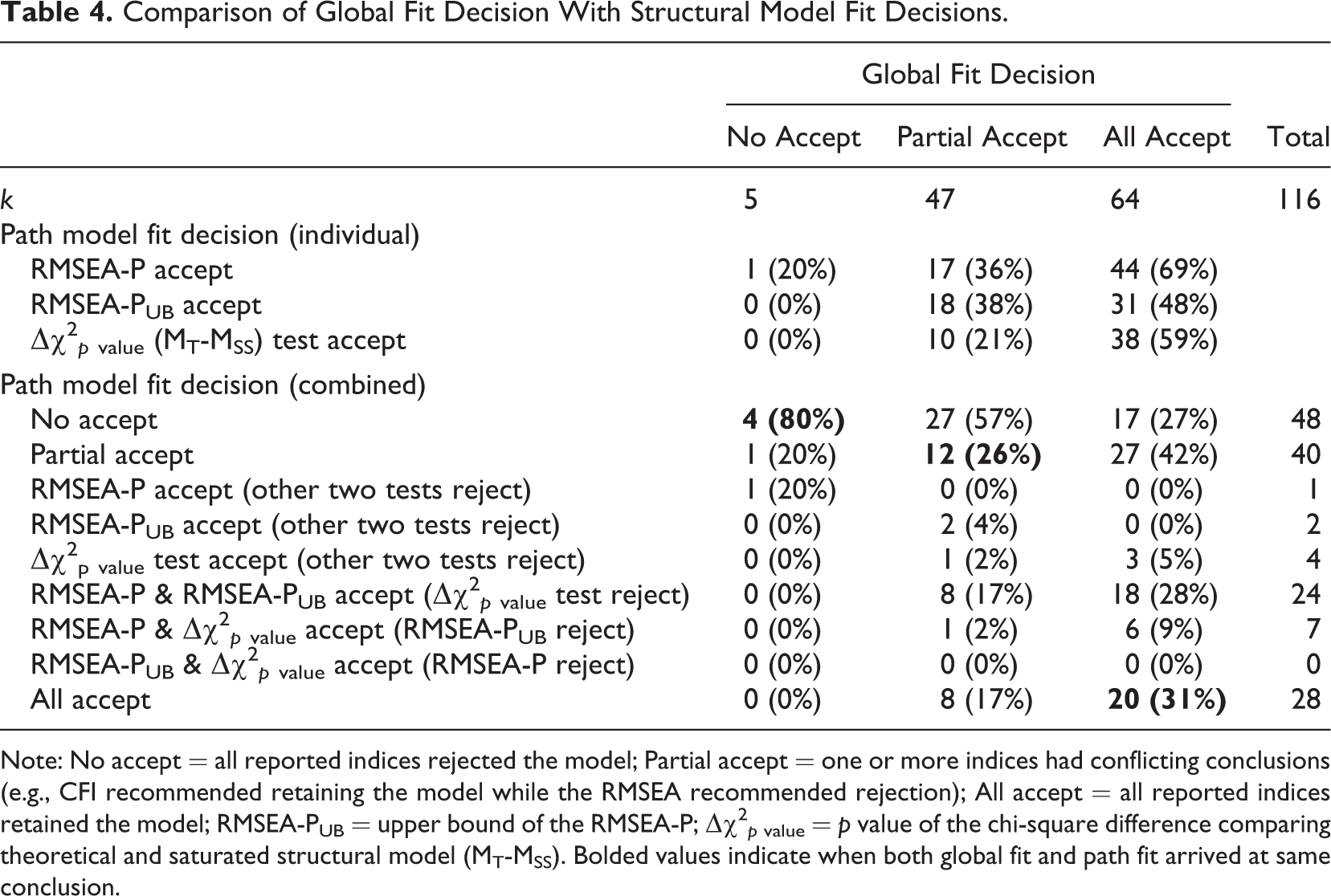
Note: No accept = all reported indices rejected the model; Partial accept = one or more indices had conflicting conclusions (e.g., CFI recommended retaining the model while the RMSEA recommended rejection); All accept = all reported indices retained the model; RMSEA-P_UB = upper bound of the RMSEA-P; Δχ² _p _value = p value of the chi-square difference comparing theoretical and saturated structural model (M_T-M_SS). Bolded values indicate when both global fit and path fit arrived at same conclusion.

As shown in the top half of Table 4, there were five studies where all reported global fit indices indicated poor global model fit. In terms of path model fit, only one of the five had an acceptable RMSEA-P, and in all five studies would not be accepted based on an upper bound of their RMSEA-P being in excess of .10 or having a statistically significant Δχ² test. Moving on to the 47 studies for which one or more but not all of the reported global fit measures met recommended threshold values, there were between 21% and 38% that were deemed to have adequate path model fit based on one of the three approaches to judging path models. Since the RMSEA-P_UB emphasizes generalization to the population and attempts to account for sampling error, we note that 18 of the 47 studies (38%) studies showed good path model fit based on this approach. Finally, there were 64 studies for which all reported global fit measures met their respective thresholds. Of these, path model fit was deemed acceptable between 48% and 69% of the time, and taking into account sampling error with the RMSEA-P_UB, path model fit was acceptable in 48% of cases.

Whereas the above results emphasize decisions based individual path model fit tools, we also examine how global fit relates to agreement among the path model fit metrics. The final set of results is presented in the lower part of Table 4 and reports how agreement among global fit values is associated with whether there is agreement among the three measures of path model fit concerns the agreement in decisions about the path model. Of the five studies where there was agreement from all reported global fit indices that their models would not be accepted, there were four for which the three path model tests were in agreement that the path should not be accepted. When the global fit indices indicated partial acceptance (k = 47), the three path indices were in agreement to not accept the path model 27 times (57%). In the cases of partial global fit acceptance, partial path model fit was found in 12 cases (26%), and the three path indices agreed to accept the path model in 8 studies (17%). For the final category of 64 studies where global fit indices agree, there were 17 studies (27%) in which all three path tests indicated not accepting the path model. For this category there were 27 studies (42%) in which two of the three paths test were supportive of the path model, and in 20 studies (31%) all three path tests indicated path model acceptance.

In sum, of the 116 studies for which we were able to conduct our analysis, complete agreement to either reject or retain the path model was achieved most of the time (k = 48 + 28 = 76 or 66%). For the 40 instances where there was conflicting results among the path model indices, 24 of these instances occurred when the RMSEA-P and the upper bound test accepted the path model and the Condition 10 M_T – M_SS chi-square difference test rejected it.

Comments, Recommendations and Future Directions for Condition 9 and 10 Assessments

Our review documented the increasing use of structural equation methods in organizational research, after tracing the roots of this use to the seminal work of James et al. (1982). Our review covers an extended time period and top micro- and macro-management journals, and extends previous work as it considers use of the three most popular global fit indices, relations of these indices with three techniques for path model assessment, and relations among the path model evaluation techniques. Our review incorporates a focus on decisions common to organizational researchers as they judge their latent variable model and decide whether their theory is supported, and how these decisions vary based on the particular index or technique used. Before proceeding to discussing key points emerging from our review, we encourage researchers to remember that the strongest case for establishing a causal relationship between an independent and dependent variable involves an experimental design, where random assignment helps eliminate alternative explanations for any observed effect. The fact that in many organizational research settings such random assignment is not possible has helped increase the reliance on statistical control and the use of path models with correlational data, allowing for development and testing of explicit causal propositions (as noted by Feldman, 1975). Within this context, the ten conditions for confirmatory analysis of James et al. have helped researchers increase the chances (but not guarantee) that obtained significant results actually reflect the causal hypotheses being examined, especially their Condition 9 and 10 tests.

A first point we would like to emphasize about these two tests concerns misconceptions about the order in which the tests should be conducted. We have encountered many substantive researchers who link model fit and significance of model paths and believe that (a) good fitting models will have significant paths, and (b) bad fitting models will have nonsignificant paths. As a result, they often focus first on whether the paths in their model are statistically significant, especially since these paths are so closely aligned with hypotheses developed in their introduction sections, and also because it is a simple binary decision (is p < .05?). Perhaps this reflects an unintended consequence of the labels of Condition 9 and Condition 10, which might be seen as suggesting they be implemented in that order. In fact, it is imperative that fulfillment of Condition 10 be established first, and it must be remembered that parameter estimates are conditional and dependent on model specification. The only scenario in which these estimates and their significance can be taken as evidence of causal processes being examined is after the adequacy of the model has been established. Said differently, fulfillment of Condition 10 is mandatory before examination of Condition 9 is attempted. To reinforce this point, we encourage researchers who have used SEM to take their final model from a given study, alter its specification (change paths) in several ways, note the degradation of fit that is likely to occur, and then examine how many of these new paths based on the poor fitting model are significant. There will likely be several that are, and in the absence of Condition 10 fulfillment, an incorrect inference would be made based on these path estimates that are biased by model misspecification.

Having reminded our readers of this, we now focus attention on the use of global fit indices for Condition 10 assessment (CFI, RMSEA, SRMR) of the overall composite model and its three components. Our results show that these three global fit indices are used much more frequently than all other approaches to composite model evaluation, and that researchers (and reviewers) are paying attention to the recommended guideline values. We cannot emphasize enough that from the beginning such values put forth by developers of these indices were only intended as guidelines. Indeed, in introducing the NFI to the social science community, Bentler and Bonett (1980) simply state, “In our experience, models with overall fit indices of less than .9 can usually be improved substantially” (p. 600). Unfortunately in many disciplines (including organizational studies) such numerical values offered have come to be taken as “gold standards” such that failure to obtain them is an automatic reason for model dismissal. In our experience we have heard from many researchers of papers being rejected because the CFI or RMSEA were slightly different (e.g., CFA = .93, RMSEA = .09) from typically cited desired values. Substantive researchers (and reviewers) need to understand that these cut off values have been developed and investigated using Monte Carlo simulation techniques (they cannot be determined analytically) and that conclusions and relevance of findings from these studies depend completely on how comparable the simulation models are to the types of models examined by substantive researchers. Moreover, in most instances this comparability is not strong and the simulation models are very simplistic (too few indicators, too few latent variables, too few causal paths, unrealistic measurement models). With this in mind we strongly encourage organizational researchers to heed the advice of West et al. (2012): “We caution readers that the reification of specific cutoff standards for the acceptance or rejection of a hypothesized model can be fraught with peril” (p. 219); “current standards for interpreting acceptable model fit are only rough guidelines; they become increasingly less reasonable as they are extrapolated to models and data further from the CFA models” (p. 220).

We would also like to draw attention to issues concerning agreement of conclusions based on the use of the three most popular measures of global fit and their cut off values. Referring again to substantive researchers we have encountered, most see these three indices as interchangeable and reflecting a unitary concept of model quality. This belief may be reinforced by the high correlations obtained among them in Monte Carlo simulation research. However, correlations with real data from our studies were much lower, likely due to the restriction of range based on only good fitting models being accepted for publication. A more favorable conclusion about agreement may be reached by examining decisions based on global fit values, and our results show that across 266 studies that used two or three indices, there was agreement to either accept or reject the model in 64% of these cases. Finally we present results for a new index of agreement, delta (Lai & Green, 2016), which perhaps showed the most favorable conclusion about agreement among the two most popular indices (CFI, RMSEA). Regardless of whether one considers these estimates of agreement to be favorable or not, researchers may likely obtain findings with their data where one index meets the standard and the other does not but is close. In this case we strongly encourage them (and reviewers of their work) to not conclude their model is “bad,” and to proceed to examine the wide range of evidence that speaks to overall model fit.

Lai and Green (2016) provide a great discussion of disagreement among fit indices, comparing it to the situation where two watches disagree about what time it is and there is no known standard to determine which is right. They note that inconsistency in fit across CFI and RMSEA measures occurs “because (a) the two indices, by design, evaluate the fit from different perspectives, (b) cutoff values are needed and are being (rightly or wrongly) used and (c) the meaning of ‘good fit’ and how it relates to fit indices are not well understood in the current literature” (p. 234). They add, “When RMSEA and CFI are inconsistent, one need not automatically disregard the model just because an index fails to meet the cut-off, nor should one retain the model by reporting only the ‘good index.’ Instead, researchers should try and explain why the indices disagree and the implications of the disagreement” (p. 234). Regarding reporting, we note that as shown in Table 2 only 89 of our 311 studies (30%) reported values for all three indices, and it appears there may be a tendency to only use or report indices that meet the cutoff standards. In terms of understanding disagreements among conclusions, Moshagen and Auerswald (2017) recently have described how results with different global fit indices can be influenced by the size of a model’s factor loadings, such that with high loadings the SRMR is more sensitive to structural misspecification, while the RMSEA is more sensitive to measurement model misspecification.

As a final point about global fit indices, we emphasize that whether there is agreement or not among conclusions about global fit of composite models, such fit is not the same as path model fit. The origins of this distinction go back many years (e.g., Mulaik et al., 1989; Sobel & Bohrnstedt, 1985), even though it has not yet become mainstream in the model evaluation literature. As noted earlier, simulation studies shed light on this distinction, especially when conducted with realistic models. Williams and O’Boyle (2011) were the first to take this approach, and found that across six representative composite examples, models with severe misspecifications yielded global fit values (CFI, RMSEA, SRMR) that would lead to these models being retained. For example, in the most extreme cases models with six and five paths incorrectly omitted had one or more mean global fit values that would lead to favorable evaluation. This pattern of results was replicated by Lance, Beck, Fan, and Carter (2016). In terms of real data, McDonald and Ho (2002) were the first to investigate empirically, and they found that in 14 studies from top psychology journals reporting adequate information for analysis, nearly all demonstrated acceptable global fit, but only a few yielded adequate path model fit. Within the organizational literature, O’Boyle and Williams (2011) found that in 43 studies from top organizational journals, 37% were supported with RMSEA-P values less than .08, 21% yielded favorable RMSEA-P confidence interval values, and 30% supported path model fit based on chi-square difference tests. In our current review with a much larger set of studies, a slightly better conclusion was reached about path model fit, in that path models were supported via the three approaches in 53%, 42%, and 41% of these studies. We hope the strength and consistency of these findings with both simulation and real data will help motivate organizational researchers to direct attention in their studies to both global fit and path model fit, with the latter playing a more dominant role given theory testing focus of most of this research. We also encourage researchers to not rely exclusively on one approach to path model fit assessment, given differences about conclusions with their use found in our review.

Steps for Improved Theory Testing and Model Evaluation

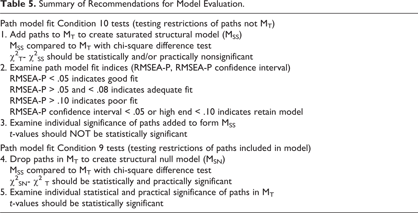
We now turn our attention to offering a set of recommendations for how organizational researchers can best evaluate their composite and path models, to demonstrate that Conditions 9 and 10 have been met. We note we are assuming that prior to implementing the steps below, the researcher has appropriately screened their data (e.g., check for normality, deal with missing data) and also thoroughly evaluated the quality of their measurement model (e.g., examine factor loadings and factor correlations). Failure to do so may lessen the effectiveness of following the recommendations below. A summary of our recommended steps for Conditions 10 and 9 assessments is provided in Table 5.

Table 5.

Summary of Recommendations for Model Evaluation.

Path model fit Condition 10 tests (testing restrictions of paths not M_T)

1. Add paths to M_T to create saturated structural model (M_SS)

M_SS compared to M_T with chi-square difference test

χ² _T- χ² _SS should be statistically and/or practically nonsignificant

2. Examine path model fit indices (RMSEA-P, RMSEA-P confidence interval)

RMSEA-P < .05 indicates good fit

RMSEA-P > .05 and < .08 indicates adequate fit

RMSEA-P > .10 indicates poor fit

RMSEA-P confidence interval < .05 or high end < .10 indicates retain model

3. Examine individual significance of paths added to form M_SS

t-values should NOT be statistically significant

Path model fit Condition 9 tests (testing restrictions of paths included in model)

4. Drop paths in M_T to create structural null model (M_SN)

M_SS compared to M_T with chi-square difference test

χ² _SN- χ² _T should be statistically and practically significant

5. Examine individual statistical and practical significance of paths in M_T

t-values should be statistically significant

Path Model Fit Condition 10

We believe the first step that should be followed involves the use of the chi-square difference test and the comparison of one’s theoretical model and a model with all possible paths (saturated structural). This comparison was emphasized by James et al. (1982) and also became the first step in a recommended series by Anderson and Gerbing (1988). This test provides direct evidence that the paths excluded from the theoretical model are not different from zero, key Condition 10 evidence. The researcher hopes to obtain a nonsignificant chi-square difference value, thus leading to a failure to reject the null hypothesis that the paths are zero, validating their exclusion. We emphasize that in spite of the prominence of this comparison in the recommendations of James et al. (1982) and Anderson and Gerbing (1988), organizational researchers most often do not include it in their model evaluation process. In fact, O’Boyle and Williams (2011) noted that among a set of 43 studies included in their review, only three conducted the test.

As for the second step with Condition 10 tests with latent variables, we note the RMSEA-P is fairly new and has not been extensively studied since originally proposed by McDonald and Ho (2002). It is commonly recommended (e.g., Chen et al., 2008) that the point-estimate of the RMSEA (and by extension RMSEA-P) be used in conjunction with its 90% confidence interval, such that a path model would be rejected if the lower bound of the confidence interval was greater than .05 or if the upper bound was greater than .10 (regardless of its point-estimate value). Its empirical performance was supported in a simulation study by Williams and O’Boyle (2011), who found that the RMSEA-P successfully distinguished between correctly and incorrectly specified models in all but one example that was atypical in that it was based on a small number of indicators per latent variable. More recently, Lance et al. (2016) reported less positive findings for the RMSEA-P, describing that with their simulation study the RMSEA-P values for moderately misspecified models (three true paths omitted) were less than .08, which would lead to these models being retained. More positive results for the RMSEA-P have been found by Williams and Williams (2017), who first reanalyzed data from Lance et al. and reached a more favorable assessment. Williams et al., then developed their own simulation data and identified fewer instances than Lance et al. in which an RMSEA-P point estimate and confidence interval resulted in support for a misspecified model. As a caveat, it is important to understand that with the RMSEA-P, due to its focus on the path component, the degrees of freedom for the path model (incorporated in the computation of the RMSEA-P) will typically be very small. Kenny, Kaniskan, and McCoach (2015) have investigated latent growth models with small degrees of freedom and found that the RMSEA may falsely indicate a poor fitting model and, they encourage researchers in such cases to not dismiss the model without considering other information. Specifically a process comparable to the third Condition 10 approach, the omitted parameter test, should be conducted.

Regarding our third step for Condition 10 assessment of latent variable relations, we begin our comments with a reminder that when it comes to path models, what you do not see is just as important as what you see. This statement reflects our belief that researchers focus on the paths they include and can see in their path diagrams, and see these as the essential hypotheses of their model. We emphasize the alternative as stated by Mulaik (2009), “Most discussions of model fit focus on how the fit of the model is a function of the estimated parameters of the model. In fact, the problem of parameter estimation so dominates these discussions that what is often lost sight of is what has been hypothesized and is to be tested in one’s model. The hypothesis is about the fixed and constrained parameters in the framework of one’s model” (p. 307). Unfortunately, the recommended approach from James et al. (and Anderson & Gerbing, 1988) of the omitted parameter test (comparing the theoretical model M_T with an alternative model that includes paths predicted to be zero-M_SS, hoping for nonsignificant path estimates) has not typically been conducted. Instead, researchers have come to rely nearly exclusively on global goodness of fit measures of the entire composite model. And this has occurred even though James et al. (1982) and Anderson and Gerbing (1988) saw global fit measures as providing information that supplemented the results of chi-square difference tests, rather than playing the dominant role that they have. As a result, the significance of these paths via the omitted parameter test has not been typically examined, and we feel they can provide important supplemental information relative to the chi-square difference test and RMSEA-P path model fit values.

In summary, for Condition 10 tests of latent variable relations, we recommend use and reporting of all three approaches: (a) chi-square difference test between theoretical and saturated path model, (b) the RMSEA-P and its confidence interval, and (c) examination of significance of paths added to implement the saturated path model. In the case of inconsistencies among results from these approaches, we support the same approach that Lai and Green (2016) recommended for disagreements between CFI and RMSEA discussed earlier. We encourage researchers to report results for all three, and attempt to determine what each reveals about their theory and what characteristics of their model and data might be leading to the differences in findings. We also believe that it should be remembered that good path model fit does not mean that the “true” representation of links between latent variables has been proven, and that determining how to revise a model with poor fit for subsequent testing with new data will not always be easy.

Path Model Fit Condition 9

For Condition 9, James et al. (1982) described a chi-square difference test comparing the theoretical model with an alternative model restricting the causal paths to zero (in which a significant difference is the goal). As shown in Table 5 we commend this test as a fourth step in path model evaluation. Its use can be seen as an approach to controlling for the risk of Type I errors involved in the next step, which can be especially relevant with larger models with many paths. The fifth and final test involves the use of significance tests of parameter estimates. In the articles in our review we observed that nearly all studies tested individually for parameter significance.

Before concluding this section it is worth noting that in their original form both Condition 9 and 10 tests rely exclusively on null hypothesis significance testing (NHST). This is consistent with the spirit of the times in 1982 where with some notable exceptions, the merits of a model, parameter, or hypothesis were not only narrowly decided by a p value, but even more narrowly decided by which side of .05 that p value fell. In the intervening three and half decades much has been learned and debated about the problematic nature of over-relying on NHST and the fallacy of equating statistical significance with practical significance. There are no clear-cut guidelines or benchmarks of what is, for example, a medium sized path coefficient in the SEM context or what is a large versus small drop in CFI as one moves from the measurement model to the structural model. However, even in the absence of hard and fast rules (which we would discourage), the magnitude of path coefficients, the variance accounted for in endogenous variables, and changes in fit indices as constraints are introduced are still important matters. We encourage researchers to build upon the traditional Condition 9 and 10 tests with some additional considerations.

First and with regard to parameter (path) estimates (Condition 9), is the effect consistent with the theoretical model and past research in terms of direction and magnitude (Edwards & Berry, 2010)? This encourages increased theoretical precision and can be evaluated a priori in terms of a non-nil hypothesis (e.g., within the proposed model specification, the standardized path from X to Y will exceed .20). Alternatively, this can be done post hoc as an area worthy of future exploration (e.g., although not hypothesized, the magnitude and counterintuitive direction of the effect, indicates a possible boundary condition to Theory X).

Second and with regard to Condition 10, the same issues will plague exclusive reliance on the statistical significance of Δχ² in model comparisons as exclusive reliance on the statistical significance of χ² as an index of model fit. A statistically significant Δχ² can be the result of (a) minor misfit across a single or small number of constrained paths coupled with a large sample size, (b) minor misfit across most or a large number of constrained paths, or (c) major misfit of a single path. Conversely, a nonsignificant Δχ² can be the result of a small sample, good fit, or some combination of both. To address the inadequacy of exclusive reliance on a single index of (mis)fit, we encourage researchers to examine the change in other valid fit indices such as the CFI, SRMR, and RMSEA. By doing so, researchers can triangulate on the extent of misfit introduced when moving from the measurement model to structural model or when moving from initial specification to respecification. Not only will this assist researchers in ultimately deciding which model to retain, it will also allow researchers to identify problematic areas in the model as certain indices can be more affected by the number of constraints in the structural model and the severity and location of misfit.

Future Research

Finally, although our article reviews themes related to Conditions 9 and 10 regarding agreement among global fit values and also new indices that focus on the path component, we note there is considerable research being conducted on model evaluation by quantitative methodologists. Although it is beyond the purpose of this article to summarize all this research, we would like to highlight a few areas that we see as promising. One line of research involves investigating how to adjust goodness of fit measures like the RMSEA and CFI for violations of the assumption of multivariate normality (Brosseau-Liard, Savalei, & Li, 2012). Given the likelihood that measures used in organizational research may not always be normally distributed, these corrections should become increasingly important. Other researchers have focused on how individual observations from a sample can impact decisions about model fit (e.g., Sterba & Pek, 2012), including those that are outliers or leveraged observations (e.g., Yuan & Zhong, 2013). The use of scatter plots to identify such problem observations has also been considered (e.g., Yuan & Hayashi, 2010). Organizational researchers also often use data that may be considered as clustered (reflecting multilevel processes) and the impact of this data property on model fit has been examined (e.g., Pornprasertmanit, Lee, & Preacher, 2014). Finally, since organizational researchers often compare competing nested models, work on issues related to statistically comparing the fit of such nested models should also be of interest (Li & Bentler, 2011).

Conclusions

It is an honor to provide this summary of the contributions of Lawrence R. (Larry) James via the seminal book James et al. (1982). The discussions of conditions for model confirmation have impacted over three decades of research based on structural equation methods. It provided a road map for researchers seeking to test causal models with nonexperimental data, and its impact will likely only continue as future generations of substantive researchers use this analytical technique.

Footnotes

Appendix

Authors’ Note

Ernest H. O’Boyle is now affiliated to Kelley School of Business, Indiana University, Bloomington, IN, USA and Jia (Joya) Yu is now affiliated to University of Nebraska–Lincoln, Lincoln, NE, USA.

Declaration of Conflicting Interests

The author(s) declared no potential conflicts of interest with respect to the research, authorship, and/or publication of this article.

Funding

The author(s) received no financial support for the research, authorship, and/or publication of this article.

References

Anderson

J. C.

Gerbing

D. W.

(1984). The effect of sampling error on convergence, improper solutions, and goodness-of-fit indices for maximum likelihood confirmatory factor analysis. Psychometrika, 49(2), 155–173.

Anderson

J. C.

Gerbing

D. W.

(1988). Structural equation modeling in practice: A review and recommended two-step approach. Psychological Bulletin, 103(3), 411–423.

Austin

P. C.

(2002). Bayesian extensions of the Tobit model for analyzing measures of health status. Medical Decision Making, 22(2), 152–162.

Bagozzi

R. P.

(1980). Causal models in marketing. New York, NY: John Wiley.

Bentler

P. M.

(1990). Comparative fit indexes in structural models. Psychological Bulletin, 107(2), 238–246.

Bentler

P. M.

(1995). EQS structural equations program manual. Encino, CA: Multivariate Software.

Bentler

P. M.

Bonett

D. G.

(1980). Significance tests and goodness of fit in the analysis of covariance structures. Psychological Bulletin, 88(3), 588–606.

Billings

R. S.

Wroten

S. P.

(1978). Use of path analysis in industrial/organizational psychology: Criticisms and suggestions. Journal of Applied Psychology, 63(6), 677–688.

Bollen

K. A.

(1990). Overall fit in covariance structure models: Two types of sample size effects. Psychological Bulletin, 107(2), 256–259.

10.

Brosseau-Liard

P. E.

Savalei

(2012). An investigation of the sample performance of two nonnormality corrections for RMSEA. Multivariate Behavioral Research, 47(6), 904–930.

11.

Chen

Curran

P. J.

Bollen

K. A.

Kirby

Paxton

(2008). An empirical evaluation of the use of fixed cutoff points in RMSEA test statistic in structural equation models. Sociological Methods & Research, 36(4), 462–494.

12.

Cohen

(1968). Multiple regression as a general data-analytic system. Psychological Bulletin, 70(6), 426–443.

13.

Darlington

R. B.

(1968). Multiple regression in psychological research and practice. Psychological Bulletin, 69(3), 161–182.

14.

Duncan

O. D.

(1975). Introduction to structural equation models. New York, NY: Academic Press.

15.

Edwards

J. R.

Berry

J. W.

(2010). The presence of something or the absence of nothing: Increasing theoretical precision in management research. Organizational Research Methods, 13(4), 668–689.

16.

Feldman

(1975). Considerations in the use of causal-correlational technique in applied psychology. Journal of Applied Psychology, 60(6), 663–670.

17.

Harris

M. M.

Schaubroeck

(1990). Confirmatory modeling in organizational behavior/human resource management: Issues and applications. Journal of Management, 16(2), 337–360.

18.

L. T.

Bentler

P. M.

(1998). Fit indices in covariance structure modeling: Sensitivity to underparameterized model misspecification. Psychological Methods, 3(4), 424–453.

19.

James

L. A.

James

L. R.

(1989). Integrating work environment perceptions: Explorations into the measurement of meaning. Journal of Applied Psychology, 74(5), 739–751.

20.

James

L. R.

Mulaik

S. A.

Brett

J. M.

(1982). Causal analysis: Assumptions, models, and data (Vol. 1). Beverly Hills, CA: Sage.

21.

Jöreskog

K. G.

Sörbom

(1979). Advances in factor analysis and structural equation models. Cambridge, MA: Abt books.

22.

Kenny

D. A.

(1979). Correlation and causality. New York, NY: John Wiley.

23.

Kenny

D. A.

Kaniskan

McCoach

D. B.

(2015). The performance of RMSEA in models with small degrees of freedom. Sociological Methods & Research, 44(3), 486–507.

24.

Khattab

Hocevar

(1982, 3). Significance testing in confirmatory factor analytic models. Paper presented at the conference of the American Educational Research Association, New York, NY.

25.

Kline

R. B.

(2015). Principles and practice of structural equation modeling. New York, NY: Guilford.

26.

Lai

Green

S. B.

(2016). The problem with having two watches: Assessment of fit when RMSEA and CFI disagree. Multivariate Behavioral Research, 51, 220–239.

27.

Lance

C. E.

(1986). Disturbance term regression test procedures for recursive and nonrecursive models: Solutions from intercorrelation matrices. Multivariate Behavioral Research, 21, 429–439.

28.

Lance

C. E.

Beck

S. S.

Fan

Carter

N. T.

(2016). A taxonomy of path-related goodness-of-fit indices and recommended criterion values. Psychological Methods, 21(3), 388–404.

29.

LeBreton

Bing

(2008). The truth(s) on testing for mediation in the social and organizational sciences. In Lance

C. E.

Vandenberg

R. J.

(Eds.), Statistical and methodological myths and urban legends: Doctrine, verity, and fable in organizational and social sciences (pp. 107–142). New York, NY: Routledge.

30.

Bentler

P. M.

(2011). Quantified choice of root-mean-square errors of approximation for evaluation and power analysis of small differences between structural equation models. Psychological Methods, 16(2), 116–126.

31.

Marsh

H. W.

Balla

J. R.

McDonald

R. P.

(1988). Goodness-of-fit indexes in confirmatory factor analysis: The effect of sample size. Psychological Bulletin, 103(3), 391–410.

32.

McDonald

R. P.

M. H. R.

(2002). Principles and practice in reporting structural equation analyses. Psychological Methods, 7(1), 64–82.

33.

Medsker

G. J.

Williams

L. J.

Holahan

P. J.

(1994). A review of current practices for evaluating causal models in organizational behavior and human resources management research. Journal of Management, 20(2), 439–464.

34.

Moshagen

Auerswald

(2017). On Congruence and Incongruence of Measures of Fit in Structural Equation Modeling. Psychological Methods. Advance online publication. https://dx-doi-org.web.bisu.edu.cn/10.1037/met0000122

35.

Mulaik

S. A.

(2009). Linear causal modeling with structural equations. Boca Raton, FL: CRC Press.

36.

Mulaik

S. A.

James

L. R.

Van Alstine

Bennett

Lind

Stilwell

C. D.

(1989). Evaluation of goodness-of-fit indices for structural equation models. Psychological Bulletin, 105(3), 430–445.

37.

O’Boyle

E. H.

Williams

L. J.

(2011). Decomposing model fit: Measurement versus theory in organizational research using latent variables. Journal of Applied Psychology, 96, 1–12.

38.

Pornprasertmanit

Lee

Preacher

K. J.

(2014). Ignoring clustering in confirmatory factor analysis: Some consequences for model fit and standardized parameter estimates. Multivariate Behavioral Research, 49(6), 518–543.

39.

Ryu

(2014). Model fit evaluation in multilevel structural equation models. Frontiers in Psychology, 5, 81.

40.

Shook

Ketchen

Hult

Kacmar

(2004). Use of structural equation modeling in strategic management research. Strategic Management Journal, 25, 397–404.

41.

Sobel

M. E.

Bohrnstedt

G. W.

(1985). Use of null models in evaluating the fit of covariance structure models. Sociological Methodology, 1985, 152–178.

42.

Steiger

J. H.

Lind

J. C.

(1980, 5). Statistically-based tests for the number of common factors. Paper presented at the annual Spring Meeting of the Psychometric Society, Iowa City, IA.

43.

Sterba

S. K.

Pek

(2012). Individual influence on model selection. Psychological Methods, 17(4), 582–599.

44.

Tanaka

J. S.

Huba

G. J.

(1984). Confirmatory hierarchical factor analyses of psychological distress measures. Journal of Personality and Social Psychology, 46(3), 621–635.

45.

Tucker

L. R.

Lewis

(1973). A reliability coefficient for maximum likelihood factor analysis. Psychometrika, 38(1), 1–10.

46.

Werts

C. E.

Linn

R. L.

(1970). Path analysis: Psychological examples. Psychological Bulletin, 74(3), 193–212.

47.

West

S. G.

Taylor

A. B.

(2012). Model fit and model selection in structural equation modeling. In Hoyle

R. H.

(Ed.), Handbook of structural equation modeling (pp. 209–231). New York, NY: Guilford.

48.

Williams

L. J.

Gavin

Hartman

(2004). Structural equation modeling methods in strategy research: Applications and issues. In Ketchen

Bergh

(Eds.), Research methodology in strategy and management (pp. 303–346). San Diego, CA: Elsevier.

49.

Williams

L. J.

Holahan

P. J.

(1994). Parsimony-based fit indices for multiple-indicator models: Do they work? Structural Equation Modeling, 1(2), 161–189.

50.

Williams

L. J.

O’Boyle

E. H.

(2011). The myth of global fit indices and alternatives for assessing latent variable relations. Organizational Research Methods, 14, 350–369.

51.

Williams

L. J.

Williams

(2017, 8). In defense of the RMSEA-P: Reconsidering results of Lance et al. (2016). Paper presented at the meeting of the Academy of Management, Atlanta, GA.

52.

Yuan

K. H.

Hayashi

(2010). Fitting data to model: Structural equation modeling diagnosis using two scatter plots. Psychological Methods, 15(4), 335–351.

53.

Yuan

K. H.

Zhong

(2013). Robustness of fit indices to outliers and leverage observations in structural equation modeling. Psychological Methods, 18(2), 121–136.