Correlation-Based Meta-Analytic Structural Equation Modeling: Effects of Parameter Covariance on Point and Interval Estimates

Abstract

More and more researchers use meta-analysis to conduct multivariate analysis to summarize previous findings. In the correlation-based meta-analytic structural equation modeling (cMASEM), the average sample correlation matrix is used to estimate the average population model. Using a simple mediation model, we illustrated that random effects covariation in population parameters can theoretically bias the path coefficient estimates and lead to nonnormal random effects distribution of the correlations. We developed an R function for researchers to examine by simulation the impact of random effects in other models. We then reanalyzed two real data sets and conducted a simulation study to examine the magnitude of the impact on realistic situations. Simulation results suggest parameter bias is typically negligible (less than .02), parameter bias and root mean square error do not differ across methods, 95% confident intervals are sometimes more accurate for the two-stage structural equation modeling approach with a diagonal random effects model, and power is sometimes higher for the traditional Viswesvaran-Ones approach. Given the increasing popularity of cMASEM in organizational research, these simulation results form the basis for us to make several recommendations on its application.

Keywords

meta-analysis structural equation modeling meta-analytic structural equation modeling

Meta-analysis is now a popular approach to review previous studies. There are three main goals of meta-analysis: to estimate the average effect size, estimate the degree of heterogeneity, and explain the heterogeneity. Meta-analysis is a powerful tool to draw conclusions systematically from previous findings. Meta-analysts can also address research questions that are difficult, if not impossible, in primary research. In the early use of meta-analysis of correlational associations, usually only the relations between two variables were examined. Most of the meta-analytic procedures were developed initially to summarize bivariate correlations between two variables. In the past two decades, more and more researchers combined meta-analysis and path analysis to test path models. This general approach is now usually denoted as meta-analytic structural equation modeling (MASEM) (M. W.-L. Cheung, 2015a; for how this approach can contribute to theory testing and development, also see Shadish, 1996). Meta-analytic path analyses have been conducted in a wide variety of organizational research (e.g., Liu, Huang, & Wang, 2014, on job search intervention; Hong, Liao, Hu, & Jian, 2013, on the mediating roles of service climate between leadership and human resources practices and customer satisfaction; Ng & Feldman, 2015, on the paths from ethical leadership through trust in leader to task performance and other outcome variables; Colquitt, LePine, & Noe, 2000, on motivation to learn; Beus, Dhanani, & Mccord, 2015, on the effects of Big Five on workplace safety). Becker and Schram (1994) called this type of synthesis the model-driven approach of meta-analysis. They argued, “many areas of research can no longer be characterized by simple main effects and bivariate relationships” (p. 375).

In the present paper, we aimed to investigate one of the goals in MASEM, namely, to estimate the average effects. In MASEM, this entails both estimating the means of the model parameters (point estimation) and forming confidence intervals for these parameters (interval estimation). As illustrated later, the estimation of the average effects is influenced by the estimation of the mean correlations and their random effects. Therefore, this aspect was also examined. In the following sections, first, we will define the random effects (RE) path model and mean correlation matrix (MCM) path model in MASEM and briefly introduce the commonly adopted approach, the correlation-based MASEM approach. Second, we will examine analytically the potential impact of the random effect in parameters, including both variation and covariation, on point and interval estimations of parameters in this approach. Third, we will present a tool for users to explore the potential impact of random effects in parameters for any path models by simulation. Fourth, we will present the reanalyses of two previous studies and compare the results. Last, a simulation study will be reported to empirically compare the performance of two common methods, the Viswesvaran and Ones (1995) approach (denoted as VOMASEM in the present paper) and the two-stage structural equation modeling approach proposed by M. W.-L. Cheung (2015a; commonly known as TSSEM) when random effect variation and/or covariation are present among population parameters.

Defining the Random Effects Path Model and Mean Correlation Matrix Path Model

In meta-analysis, there are two main models: fixed effects model and random effects model. In the fixed effects model (Hedges & Vevea, 1998), it is assumed that the population effect is the same for all studies in an analysis. Variation in effects is due to sampling error only. This model is usually unrealistic and perhaps plausible only when the studies are identical in many aspects, such as sample characteristics, operationalization of variables, and procedures. As concluded by Hedges (2016), “heterogeneity among research results is a normative feature of science” (p. 210). Therefore, we will focus on the second major model, the random effects model (Hedges & Vevea, 1998). In the random effects model, it is assumed that there are generally two sources of variation for the effect sizes. One is sampling error. The other is genuine variation in the population effect sizes. This variation, usually denoted as the random effect, can be due to many other factors, such as research artifacts and theoretically meaningful study characteristics. The latter are usually called moderators in meta-analysis (Schmidt & Hunter, 2015). Despite this variation in population effect sizes in the random effects model, it is still informative to estimate the average of the population effect size. Therefore, one goal in the random effects model is to estimate the average effect.

In MASEM, with three or more variables involved, it is reasonable to expect that the fixed effects model is even less plausible than it is in the meta-analysis of a bivariate relation (between two continuous variables as in correlation or between a categorical variable and a continuous variable as in standardized mean difference). However, how a mean model under a random effects model is defined has rarely been discussed in MASEM.

If all variables were measured in all studies in a MASEM review, one can use parameter-based MASEM (M. W.-L. Cheung & Cheung, 2016). A model is fitted to all studies, and the parameter estimates from these studies are then treated as effect sizes and meta-analyzed as usual using techniques for multivariate meta-analysis. Random effect in parameter estimates can be estimated directly. We do not need any techniques specifically for MASEM. We denote this model as the RE path model. This is similar to a usual path model except that it has two sets of parameters: the means of the model parameters and random effects variance and covariances of the model parameters. This is a direct extension of the random effects model in conventional meta-analysis except that instead of one mean and one “true” variance, there are more than one of each. It is also similar to multivariate meta-analysis except that the effect sizes are model parameters rather than simply correlated effect sizes.

For example, suppose we are going to do a meta-analysis on three variables: attitude, intention, and behavior. One possible RE path model is a complete mediation model in which attitude affects intention and intention affects behavior. In standardized form, this model has two free parameters, the standardized regression coefficients from attitude to intention, denoted as a, and the standardized regression coefficients from intention to behavior, denoted as b. These two free parameters are allowed to be any valid values, including zero, in the population. The path from attitude to behavior is fixed to zero in all studies. That is, the RE path model posits that this direct path is zero for all studies in the population. It has two free random parameters (a and b), with population means, random effects variances, and random effects covariances. Let us denote this as RE path Model 1, as illustrated in Figure 1. Another example is a partial mediation model, denoted as RE path Model 2 in Figure 1, with three standardized parameters, all allowed to vary across studies and may covary among themselves. It has three free random parameters (a, b, and the direct path, denoted as c’), with three population means and a three-by-three random effects variance-covariances matrix. By parameter-based MASEM, both models may be fitted in all studies, and the hypothesis that intention fully mediates the effect of attitude on behavior in all studies is tested empirically. For example, we can test whether the mean and random effect variance of the direct path are both nonsignificant. If yes, then the data favor RE path Model 1. If the mean of the direct path is not significant but the random effect variance is significant, then the data favor RE path Model 2.

Figure 1.

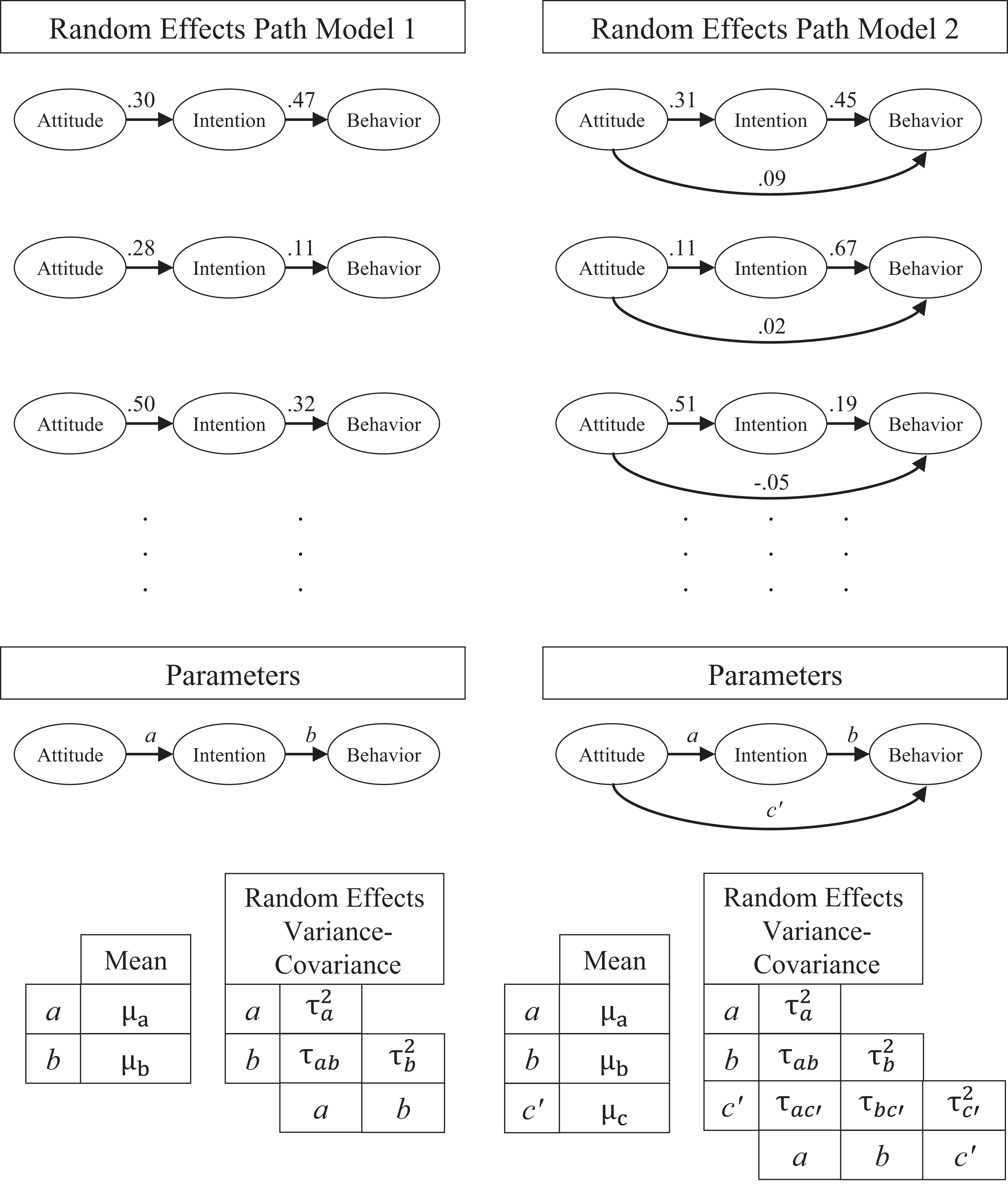
Examples of random effects (RE) path models.

Unfortunately, parameter-based MASEM is rarely feasible in practice. It is common that for a model of interest, very few studies measured all variables in the model. It is also undesirable to exclude studies that measured some but not all the variables. Therefore, the common practice is to form an average correlation matrix based on available information and then test one or more models on this average correlation matrix. We denote this model in correlation-based MASEM as the MCM path model. This approach is called the correlation-based MASEM approach (M. W.-L. Cheung & Cheung, 2016; denoted as cMASEM in the following) and is the dominant approach in MASEM.

Correlation-Based MASEM

All common approaches within cMASEM, except for the full-information MASEM (FIMASEM) proposed by Yu, Downes, Carter, and O’Boyle (2016; to be reviewed later), involve two stages. First, an average sample correlation matrix is computed. Second, a path model, called MCM path model in the present paper, is fitted to this correlation matrix. The common approaches differ on the procedures used in these two stages. In the VOMASEM approach (proposed by Viswesvaran & Ones, 1995), each bivariate relation is meta-analyzed separately to form the average sample correlation matrix. For example, with four variables and hence six bivariate relations, six meta-analyses will be conducted. The average sample correlations from these meta-analyses will then be used to form the average sample correlation matrix (e.g., Premack & Hunter, 1988; Viswesvaran, Schmidt, & Ones, 2005). Approaches similar to this one were used as early as the 1980s (e.g., Premack & Hunter, 1988) but are still popular nowadays in organizational research (see e.g., Beus et al., 2015; Courtright, Thurgood, Stewart, & Pierotti, 2015; Knight & Eisenkraft, 2014). In the generalized least squares approach (GLS; Becker, 1992, 1995; see e.g., Ouellette & Wood, 1998) or the multilevel approach (Kalaian & Raudenbush, 1996; Raudenbush, Becker, & Kalaian, 1988), all the available sample correlations are jointly analyzed using a regression model, with the correlations as dependent variables, to compute the average sample correlation matrix. In the TSSEM approach (M. W.-L. Cheung, 2015a; M. W.-L. Cheung & Chan, 2005), structural equation modeling (SEM) is used to estimate the average sample correlation matrix. These approaches differ in their assumptions and estimation. However, all approaches basically come up with a correlation matrix that is intended for estimating the population correlation matrix or the average population correlation matrix in cases of heterogeneity (see the next section). In this stage, some procedures use random effects model. For example, if the Hunter-Schmidt procedure is used, the correlations in each cell of the correlation matrix may be tested for homogeneity and the variation of population correlations estimated (e.g., Joseph, Jin, Newman, & O’Boyle, 2015). It is also possible to adopt an RE model in GLS and TSSEM when forming the average sample correlation matrix.

After the average sample correlation matrix has been computed, a path model or a structural model with one or more latent factors is fitted to the matrix. In VOMASEM, the average correlations in the matrix usually do not have the same total sample size due to missing data (correlations not reported or variables not measured in some studies). A number (e.g., harmonic mean, median) is selected to be the representative sample size, and then the average sample correlation matrix along with this sample size are submitted to an SEM program as if the matrix were from a single large sample. Though rarely stated clearly in studies using VOMASEM, it seems that the mean correlation matrix is usually treated as a covariance matrix when fitting a model. In the GLS, multilevel, and TSSEM approaches, the sampling variance-covariance of the correlations can be estimated and used in SEM programs directly instead of the sample size. Although these cMASEM approaches differ on how to implement the second stage, they basically estimate the population parameters as in typical structural equation modeling, with differences in modeling the sampling variances and covariances.

To the best of our knowledge, all the common procedures mentioned previously do not make use of the random components in Stage 2 even though random effects are modeled when computing the mean correlation matrix in the first stage. All model parameters in Stage 2 are assumed to be fixed. In other words, a fixed effects model is actually adopted in Stage 2 of cMASEM. For example, in their meta-analysis of Big Five’s effects on workplace safety, Beus et al. (2015) found non-negligible random effects for correlations between some variables in the first stage, and moderators such as study context and age were used to explain such heterogeneity. However, in the second stage, when fitting the mediation model, the correlations were treated as homogeneous, and the path model was interpreted as in primary studies, with no random effects. This is a common practice for other similar MASEM studies (e.g., Joseph et al., 2015; Ng & Feldman, 2015; but see Knight & Eisenkraft, 2014, which used subgroup analysis in Stage 2 to investigate possible impact of moderators on path coefficients). In a review by Sheng, Kong, Cortina, and Hou (2016) of cMASEM studies (they did not use the term cMASEM, but most of studies they identified used methods in this category), many studies did not include moderators when testing path models in Stage 2. This is conceptually inconsistent because on the one hand, heterogeneity is found and interpreted in the correlation matrix, but on the other hand, this heterogeneity is ignored when testing and interpreting the model fitted to the correlation matrix.

To take into account heterogeneity in model parameters implied by heterogeneity in the correlation matrices, Yu et al. (2016) proposed the FIMASEM method. Although they used VOMASEM (denoted as traditional MASEM in their paper) and TSSEM (and they denoted the application of FIMASEM to TSSEM as TS-FIMASEM), in principle, FIMASEM can be applied to all cMASEM approaches that yield both a mean correlation matrix and an estimate of the random effects in the correlation matrix. In addition to fitting a model to the mean correlation matrix, a large number of random correlation matrices are generated, using a normal distribution with means equal to the mean correlation matrix and standard deviations equal to the random effects estimated in Stage 1. The hypothesized model is then fitted to each of these random correlation matrices. The heterogeneity in model parameters is examined through the distribution of the model parameters from simulated correlation matrices. Heterogeneity in goodness of fit can be similarly investigated.

The FIMASEM is a promising extension to fill the gap of estimating the degree of heterogeneity of model parameters in cMASEM without the need for parameter-based MASEM. However, it is still an emerging approach that needs more empirical studies. Moreover, similar to other cMASEM approaches, it relies on the accuracy of the Stage 1 results, that is, the estimation of the mean correlation matrix and its random effects. The focus of the present study is on Stage 1 and its impact on Stage 2. Therefore, we will not further investigate FIMASEM in the present study.

Estimation in cMASEM

Two issues on estimation will be investigated in the following sections. First, we will examine to what extent the parameter estimates of the MCM path model fitted in cMASEM can provide unbiased point and interval estimates of the means of the parameters in the RE path model. Despite the lack of techniques for estimating random effects directly in the second stage of cMASEM, one can argue that this approach can still estimate parameters in the RE path model. Moreover, if random effects in the correlation matrix have been accounted for in Stage 1, one can argue that the Stage 2 confidence intervals should have taken into account random effects in model parameters. The assumption that cMASEM estimates parameter means in the RE path model is required when researchers acknowledge random effects in Stage 1 but then interpret the model parameters as fixed in Stage 2. For example, in Hong et al.’s (2013) investigation of the effect of service climate on customer satisfaction and financial outcomes through proposed mediators, they found that service contexts (personal service vs. nonpersonal service) did significantly moderate the correlations between service climate and some of the mediators as well as outcome variables. Nevertheless, researchers can defend this approach by arguing that the Stage 2 path analysis results can still estimate the average direct and indirect effects of service climate on the outcome variables.

The issues that we will investigate in the following are not confined to any particular implementation of the cMASEM approach. We would like to examine whether cMASEM can in principle unbiasedly estimate the parameter means of the RE path model if: (a) the model being fitted in Stage 2 is not misspecified, (b) both the number of studies and the sample sizes of the studies are large, and (c) all studies provided the full correlation matrix (i.e., no missing correlation). We will show that even under these ideal conditions, things can go wrong. Therefore, in the next section, we will not focus on any particular implementation of cMASEM approach.

Example: A Simple Mediation Model

We will use a simple mediation model as an example and examine how parameter variation and covariation may affect the implied population correlations. This model has three variables, X (independent variable), M (mediator), and Y (dependent variable). The effect of X on M is a, the effect of M on Y is b, and the direct effect from X to Y is c’. Under random effects model, these parameters may vary and/or covary. The implied population correlations are

ρ_{M X} = a

ρ_{Y X} = c' + a b

ρ_{Y M} = b + a c'

Table 1 shows the expectations, random effect variances, and random effect covariances of the implied population correlations (derived in Online Appendix A). In these equations, μ_U denotes the expected value of u, $τ_{U}^{2}$ denotes the variance of u, and τ_UV denotes the covariance of u and v. Note that these are the variances and covariances of the population parameters across studies, not sampling variances or covariances.

Table 1.

Expectations, Variances, and Covariances of Implied Correlations.

	Expectation			Variance			Covariance
Model	ρ_MX	ρ_YX	ρ_YM	ρ_MX	ρ_YX	ρ_YM	$(ρ_{M X}, ρ_{Y X})$	$(ρ_{M X}, ρ_{Y M})$	$(ρ_{Y X}, ρ_{Y M})$
All parameters vary and covary	μ_a	$μ_{c^{'}} + μ_{a} μ_{b} + τ_{a b}$	$μ_{b} + μ_{a} μ_{c^{'}} + τ_{a c^{'}}$	$τ_{a}^{2}$	$μ_{b}^{2} τ_{a}^{2} + μ_{a}^{2} τ_{b}^{2} + τ_{c^{'}}^{2} + τ_{a}^{2} τ_{b}^{2} + 2 μ_{a} μ_{b} τ_{a b} + {(τ_{a b})}^{2} + 2 μ_{b} τ_{a c^{'}} + 2 μ_{a} τ_{b c^{'}}$	$μ_{c}^{2} τ_{a}^{2} + μ_{a}^{2} τ_{c ′}^{2} + τ_{b}^{2} + τ_{a}^{2} τ_{c ′}^{2} + 2 μ_{a} μ_{c ′} τ_{a c ′} + {(τ_{a c^{'}})}^{2} + 2 μ_{c ′} τ_{a b} + 2 μ_{a} τ_{b c ′}$	$μ_{b} τ_{a}^{2} + μ_{a} τ_{a b} + τ_{a c^{'}}$	$μ_{c ′} τ_{a}^{2} + τ_{a b} + μ_{a} τ_{a c ′}$	$μ_{b} μ_{c ′} τ_{a}^{2} + μ_{a} τ_{b}^{2} + μ_{a} τ_{c ′}^{2} + (μ_{b} + μ_{a} μ_{c ′}) τ_{a b} + (μ_{c ′} + μ_{a} μ_{b}) τ_{a c ′} + (1 + μ_{a}^{2} + τ_{a}^{2}) τ_{b c ′} + τ_{a b} τ_{a c ′}$
All parameters vary but uncorrelated	μ_a	$μ_{c ′} + μ_{a} μ_{b}$	$μ_{b} + μ_{a} μ_{c ′}$	$τ_{a}^{2}$	$μ_{b}^{2} τ_{a}^{2} + μ_{a}^{2} τ_{b}^{2} + τ_{c ′}^{2} + τ_{a}^{2} τ_{b}^{2}$	$μ_{c}^{2} τ_{a}^{2} + μ_{a}^{2} τ_{c ′}^{2} + τ_{b}^{2} + τ_{a}^{2} τ_{c ′}^{2}$	$μ_{b} τ_{a}^{2}$	$μ_{c ′} τ_{a}^{2}$	$μ_{b} μ_{c ′} τ_{a}^{2} + μ_{a} τ_{b}^{2} + μ_{a} τ_{c ′}^{2}$
Example 1: $μ_{a} = .40$ , $μ_{b} = .30$ , $μ_{c^{'}} = .00$ . Parameters vary ( $τ_{a}^{2}$ , $τ_{b}^{2}$ , and $τ_{c ′}^{2}$ > 0) but uncorrelated ( $τ_{a b} = τ_{a c ′} = τ_{b c ′} = 0$ )
	.40	.12	.30	$τ_{a}^{2}$	$.09 τ_{a}^{2} + .16 τ_{b}^{2} + τ_{c^{'}} + τ_{a}^{2} τ_{b}^{2}$	$.16 τ_{c ′}^{2} + τ_{b}^{2} + τ_{a}^{2} τ_{c ′}^{2}$	$.30 τ_{a}^{2}$	.00	$.40 (τ_{b}^{2} + τ_{c ′}^{2})$
Example 2: $μ_{a} = .40$ , $μ_{b} = .30$ , $μ_{c^{'}} = .00$ . Parameters vary ( $τ_{a}^{2}$ , $τ_{b}^{2}$ , and $τ_{c'}^{2}$ > 0) and covary (τ_ab, $τ_{a c'}$ , and $τ_{b c'}$ ≠ 0)
	.40	$.12 + τ_{a b}$	$.30 + τ_{a c ′}$	$τ_{a}^{2}$	$.09 τ_{a}^{2} + .16 τ_{b}^{2} + τ_{c^{'}} + τ_{a}^{2} τ_{b}^{2} + .2 τ_{a b} + {(τ_{a b})}^{2} + .60 τ_{a c^{'}} + .80 τ_{b c^{'}}$	$.16 τ_{c ′}^{2} + τ_{b}^{2} + τ_{a}^{2} τ_{c ′}^{2} + {(τ_{a c^{'}})}^{2} + .80 τ_{b c ′}$	$.30 τ_{a}^{2} + .40 τ_{a b} + τ_{a c ′}$	$τ_{a b} + .40 τ_{a c ′}$	$.40 (τ_{b}^{2} + τ_{c ′}^{2}) + .30 τ_{a b} + .12 τ_{a c ′} + (1.16 + τ_{a}^{2}) τ_{b c ′} + τ_{a b} τ_{a c ′}$

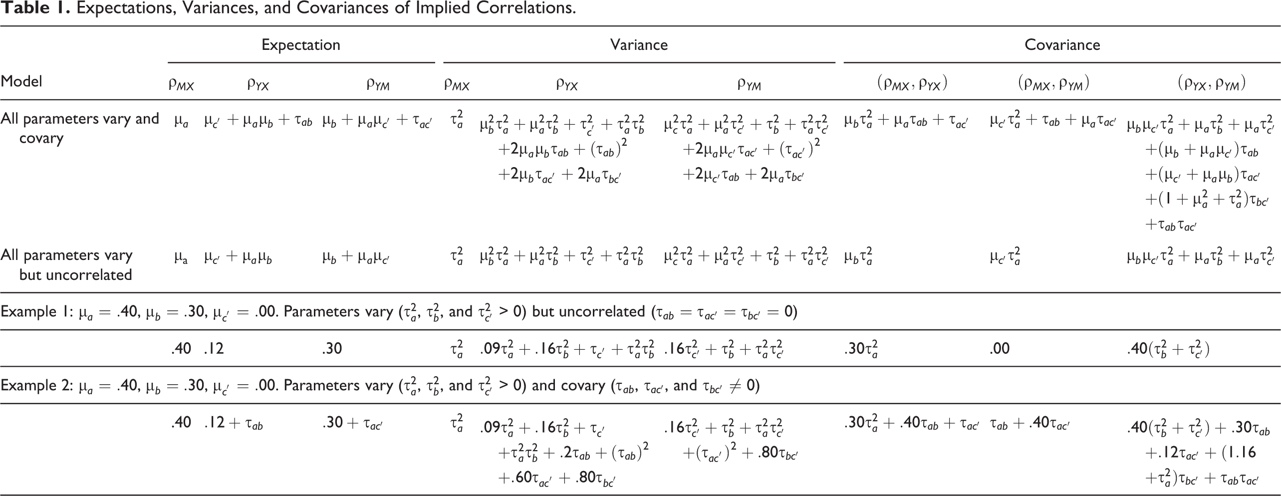
Table 1 also shows the case in which the model parameters vary but do not covary. Three observations need to be discussed. First, the expectations of two implied population correlations, ρ _YX and ρ _YM , depend on the random effect covariances among parameters (τ _ab and τ _ac′ , respectively). To the extent that a covary with b or c’, the expectation of these correlations may be different from those when the parameters have zero random effect covariances. Second, even if the parameters vary but have zero random effect covariances, the implied population correlations may still have nonzero random effect covariances (see the last three columns in Table 1). In this mediation model, the three implied population correlations have zero random effect covariances only for some combinations of the expectations and random effect variances of the model parameters, such as μ _b = μ _c’ = 0 and $τ_{b}^{2}$ = $τ_{c'}^{2}$ = 0 (the effects of X and M on Y are fixed to zero) or μ _a = 0 and $τ_{a}^{2}$ = 0 (the effect of X on M is fixed to zero). Third, the implied population correlations ρ_YX and ρ_YM are the sum of a model parameter and the product of two other model parameters (ab and ac′, respectively). It is well known that the distribution of ab is nonnormal even if a and b are normally distributed (Craig, 1936; but note that the distribution of ab can approach a normal distribution in some special cases; see Aroian, 1947). However, to the extent that the other component (c’ in ρ _YX and b in ρ _YM ) is normally distributed, the implied population correlation may still be approximately normally distributed, especially when the variance of the other component is large and hence dominates the random effect variation of the implied population correlation. In sum, even if the random effects of the model parameters have a multivariate normal distribution, whether the random effects distribution of these two implied population correlations is approximately multivariate normal depends on the random effect variances and covariances of the random parameters.

In the following sections, we first investigate the possible impact of random effect variation without covariation on parameter estimation. We then examine the case with both random effect variation and covariation. Numerical examples will be used to help understand the practical impact of the random effect variances and covariances.

Parameters Vary but No Random Effect Covariation

First, we consider the case when the population parameters vary across studies but the random effect covariances among population parameters are zero across studies. The simple mediation model mentioned previously is used as an example. Let’s assume in the population, attitude (X) causes intention (M), and intention causes behavior (Y). Suppose the mean of a path (attitude to intention) is .40, the mean of b path (intention to behavior) is .30, and the mean of the c’ path (attitude’s direct effect on behavior) is zero. The expectations, random effect variances, and random effect covariances of the implied population correlation are shown in Table 1, Example 1. The equations suggest three implications on cMASEM. First, had a mediation model been fitted to the expected correlation matrix, the means of the effects of attitude and intention on behavior could be recovered (a = .40, b = .30, and c’ = .00) regardless of the random effect variances of the parameters. This suggests that in this model, if the model parameters have no random effect covariation, we can safely assume that cMASEM can yield unbiased estimates of the mean parameters as long as it can unbiasedly estimate the mean correlations.

Second, unless $τ_{a}^{2}$ and either $τ_{b}^{2}$ or $τ_{c'}^{2}$ (or both) are equal to zero (i.e., the effect of attitude on intention is fixed and either the effect of intention to behavior or the direct effect, or both, is fixed), at least one of the random effect covariances between implied population correlations is nonzero. To numerically illustrate the impact, let’s consider the correlation between ρ_MX and ρ_YX ( $R_{ρ_{M X}, ρ_{Y X}}$ ) and between ρ_YX and ρ_YM ( $R_{ρ_{Y X}, ρ_{Y M}}$ ),

R_{ρ_{M X}, ρ_{Y X}} = .30 τ_{a}^{2} / \sqrt{τ_{a}^{2} (.09 τ_{a}^{2} + .16 τ_{b}^{2} + τ_{c'}^{2} + τ_{a}^{2} τ_{b}^{2})}

R_{ρ_{Y X}, ρ_{Y M}} = .40 (τ_{b}^{2} + τ_{c'}^{2}) / \sqrt{(.09 τ_{a}^{2} + .16 τ_{b}^{2} + τ_{c'}^{2} + τ_{a}^{2} τ_{b}^{2}) (16 τ_{c'}^{2} + τ_{b}^{2} + τ_{a}^{2} τ_{c'}^{2})}

Suppose $τ_{a}^{2}$ = $τ_{b}^{2}$ = $τ_{c'}^{2}$ . If the standard deviation of a ( $τ_{a}$ ) is .05, $R_{ρ_{M X}, ρ_{Y X}}$ = .268 and $R_{ρ_{Y X}, ρ_{Y M}}$ = .663. If the direct path is fixed to zero ( $τ_{c'}^{2}$ = 0) and only a and b path vary (and $τ_{a}^{2}$ = $τ_{b}^{2}$ ), with the standard deviation of a equal to .05, $R_{ρ_{M X}, ρ_{Y X}}$ = .597 and $R_{ρ_{Y X}, ρ_{Y M}}$ = .796, even larger than those with c’ also varies. That is, for a simple mediation model, even if we believe the paths have small random effects but do not covary, we should usually expect nonzero random effect covariation in the correlations, which are estimated in Stage 1 of cMASEM. If the random effect covariation is fixed to zero in Stage 1 of cMASEM, the estimates of random effect variances may be biased, resulting in biased estimates of sampling variances and covariances of model parameters in Stage 2 and affecting the confidence intervals, statistical power, and Type I error in this stage.

This is a potential problem in cMASEM because it is sometimes necessary to assume in Stage 1 that the population correlations vary but do not covary. It is because the number of elements in the random effect covariance matrix increases exponentially with the number of variables. For three variables, as in a simple mediation model, there are 3 correlations and hence 6 random effects variances and covariances for these 3 correlations. For five variables, as in the popular theory of planned behavior (Ajzen, 1991), there are 10 correlations and hence 55 variances and covariances. Even in meta-analysis, there may not be enough data to reliably estimate this large random effect covariance matrix (M. W.-L. Cheung, 2015a, Example 7.6.1.3). To the extent that some correlations covary, as in the aforementioned case, fitting a diagonal random effects model can result in biased estimates of the covariance matrix used in the second stage and confidence intervals that tended to be too narrow or too wide. This is analogous to using a fixed effect model to meta-analyze correlations when the true variance is nonzero, resulting in biased estimates of the sampling variance of the mean correlation.

Third, the random effects distribution of the three implied population correlations may deviate from a multivariate normal distribution. However, the deviation is typically small. As an example, we randomly generated 5,000 sets of a, b, and c’ with means equal to .40, .30, and .00, respectively, normally distributed but uncorrelated. The distribution of ρ _YX is close to a normal distribution, with skewness only .06 and excess kurtosis only .06.

Parameters Vary and Covary

Next, we consider a case with random effect covariation among model parameters. The same simple mediation model is used, with mean a = .40, mean b = .30, and mean c’ = .00, and all three parameters vary and covary. The expectations, variances, and covariances of the implied population correlations were shown in Table 1, Example 2. The equations suggest three implications. First, different from the case of no random effect covariation, the expectations of the three implied population correlations depend on the random effects covariances (τ_ab and $τ_{a c'}$ ). If the random effects of the three parameters are .05 in standard deviation and the random effect correlations between a and b, a and c’, and a and c’ are all equal to .10, the expectations of ρ _YX and ρ _YM are .1203 and .3003, respectively. If the random effect correlations are .80, the expectations of ρ _YX and ρ _YM are .1220 and .3020, respectively. Had a mediation model been fitted to the expected population correlation matrix, the estimate of b path and c’ path would be .3002 and .0002 for random effect correlations of .10 and .3014 and .0013 for random effect correlations of .80. This is because the biases in the expectations are equal to the random effect covariances, which are bounded by the random effect variances. For example, if the random effect SD is .05, the random effect variance is .0025, and the maximum possible random effect covariance cannot exceed .0025. Even if the random effect variation is .15, with a random effect correlation of .80, the estimates of b and c’ paths will be .3129 and .0118, not much different from .30 and .00, the means of b and c’. Nevertheless, if the random effect variation is .20 and the random effect correlation is .80, then the estimates of b and c’ paths will be .3229 and .0209, a bias of .02. In sum, if the model parameters covary, the Stage 2 cMASEM estimates of the mean model parameters will be biased, but the magnitude of the bias will depend on the random effect variation and covariation of the model parameters. In some situations, it can be practically negligible.

Second, the implied population correlations have nonzero random effects covariances. Because the terms are additive, unless one or more random effect covariances are negative, the random effects covariances for the implied population correlations will only be larger than those in the case of variation without covariation. Therefore, we will not repeat the numerical illustration here. Similar to Example 1, fitting a diagonal random effect matrix in Stage 1 of cMASEM may adversely affect the confidence intervals and statistical tests of model parameters in Stage 2.

Third, the random effect distribution may deviate from a multivariate distribution but typically only slightly, as in the case of variation without covariation (Example 1).

An R Function to Explore the Distribution of Implied Population Correlations in Other Models

Although most of the results in the simple mediation discussed previously can be derived analytically, it becomes much more complicated even in a model with four or more variables, such as a parallel mediation model with two mediators. Even with two mediators, the variances and covariances of some implied population correlations involve the expectations of the product of the deviation from the means of three variables and can no longer be simplified to variances and covariances as we did in the previous model. Moreover, the assumption of normal distribution may no longer be tenable for more complicated models. As the number of variables increases, the probability of generating an invalid correlation matrix (one that is nonpositive definite) increases, resulting in rejection of some configurations of model parameters. For example, for a three-predictor regression model, assuming that all three predictors are uncorrelated, it is impossible to have all three standardized coefficients equal to .60 because this will result in a negative implied error variance of the standardized outcome variable (–.08). In other words, the multivariate distribution of the standardized parameters is bounded, resulting in a truncated multivariate normal distribution (Tallis, 1961). This will cast doubt on the appropriateness of the simplification we did for the simple mediation model. In short, it is impractical to require researchers to explore a model analytically as we did if the models of interest have four or more variables.

One possible alternative to explore the impact of random effects in parameters on the implied population correlations is by simulation. We developed a function in R 3.3.3 (R Development Core Team, 2017) to facilitate researchers to explore path models more complicated than the simple mediation model we discussed previously. We described how to use this function in Online Appendix B.

It is beyond the scope of the present paper to examine other models. Scripts for some sample models are available from the link in Online Appendix B to illustrate how the function can be used to explore models such as a mediation model with three mediators in parallel or in serial and a regression model with three correlated predictors. The function, though in early development, can serve as a template for researchers to adapt for models of concern in their studies.

Reanalyzing Two Real Data Sets

The previous discussion is based on hypothetical cases. It is not clear how large random effect variances and covariances can be in real MASEM data sets and how much the choice of random effect model in Stage 1 can affect Stage 2 results in cMASEM. To explore the magnitude of random covariation and the potential impact of the inclusion or exclusion of random effect covariation in modeling random effects, we reanalyzed two data sets provided in metaSEM, the R package commonly used for TSSEM (M. W.-L. Cheung, 2015b). These two data sets were also analyzed in M. W.-L. Cheung and Cheung (2016), though their focus was on the differences between cMASEM and parameter-based MASEM rather than random effects per se.

The first data set is a collection of 50 correlation matrices from studies investigating the theory of planned behavior (TPB; Ajzen, 1991), reported in S.-F. Cheung and Chan (2000). Only four variables in the model were included: attitude toward a behavior (ATT), subjective norm regarding the behavior (SN), behavioral intention to perform the behavior (BI), and the performance of the behavior (BEH). Some studies did not measure all four variables. The mean and median sample sizes were 163.6 and 131, respectively. The model to be examined is a complete mediation model, with ATT and SN affect BEH through the mediator BI.

The second data set consists of 46 correlation matrices of life satisfaction (LS), job satisfaction (JS), and job autonomy (JA) obtained from 42 nations (WVS; World Value Survey Group, 1994). All correlation matrices included these three variables. The mean and median sample sizes were 849.1 and 866, respectively. The model to be examined is a complete mediation model, with JA affects LS through the mediator JS.

For each data set, two sets of TSSEM analysis were conducted; one modeled both random effect variances and covariances (full RE model), and the other modeled only random effect variances (diagonal RE model), assuming that the correlations do not have random effect covariation. The R scripts along with the results are available at Open Science Framework (https://osf.io/n2a5b/?view_only=06e7bc3045234fa9a27f73861ee6725b).

We first examined the degree of random effect covariation, available only in full RE model. For the ease of interpretation, the matrices of random effects were converted to correlation matrices such that the random covariation can be interpreted as correlations rather than covariances. As shown in Table 2, for the TPB data set, the estimated random correlation ranged from .062 to .758 in magnitude, mean = .303, and median = .385. For the WVS data set, there are only three random correlations, ranging from .201 to .823, mean = .456, larger than that in the TPB data set. This suggests that in real data sets, the random covariation between correlations can be moderate or larger when presented as correlations.

Table 2.

Estimates of Random Covariation by Full Random Effects Model, Converted to Correlation (ρ).

S. F. Cheung and Chan (2000)
	ATT ∼∼ SN	ATT ∼∼ BI	ATT ∼∼ BEH	SN ∼∼ BI	SN ∼∼ BEH	BI ∼∼ BEH
ATT ∼∼ SN	1.000
ATT ∼∼ BI	.385	1.000
ATT ∼∼ BEH	–.062	.535	1.000
SN ∼∼ BI	.758	.468	.044	1.000
SN ∼∼ BEH	.222	.184	.663	.393	1.000
BI ∼∼ BEH	–.228	.129	.660	–.128	.519	1.000
World Value Survey
	LS ∼∼ JS	LS ∼∼ JA	JS ∼∼ JA
LS ∼∼ JS	1.000
LS ∼∼ JA	.823	1.000
JS ∼∼ JA	.201	.344	1.000

Note: ATT = attitude; SN = subjective norm; BI = behavioral intention; BEH = behavior; LS = life satisfaction; JS = job satisfaction; JA = job autonomy. X ∼∼ Y denotes the correlation between X and Y.

We then examined the mean correlations estimated by full and diagonal RE models. Table 3 shows that the differences in point estimates are negligible, with magnitude .01 or less except for two correlations in the TPB data set (largest difference = .025). This suggests that the choice of RE model may have little impact on point estimation of the mean correlations.

Table 3.

Estimates of Mean Correlations by Diagonal Random Effects or Full Random Effects.

	ATT ∼∼ SN	ATT ∼∼ BI	ATT ∼∼ BEH	SN ∼∼ BI	SN ∼∼ BEH	BI ∼∼ BEH
S. F. Cheung and Chan (2000)
Full	.358	.486	.274	.309	.134	.439
Diagonal	.359	.476	.299	.300	.149	.435
Diff	.001	–.010	.025	–.009	.014	–.004
	LS ∼∼ JS	LS ∼∼ JA	JS ∼∼ JA
World Value Survey
Full	.369	.216	.435
Diagonal	.369	.217	.434
Diff	.000	.001	–.001

Note: Diff = the difference in estimate or confidence interval (CI) width between diagonal random effects results and full random effects results (diagonal – full); ATT = attitude; SN = subjective norm; BI = behavioral intention; BEH = behavior; LS = life satisfaction; JS = job satisfaction; JA = job autonomy. X ∼∼ Y denotes the correlation between X and Y.

Table 4 shows the estimated random effects variances for the correlations being meta-analyzed, available in both diagonal and full RE models. For the ease of interpretation, the random effects were presented as standard deviations. In terms of magnitude, the differences are small, ranging from .002 to .020 in magnitude. However, for both data sets and all correlations, the estimates by the diagonal RE model were consistently lower than those by the full RE model.

Table 4.

Random Effects by Diagonal Random Effects or Full Random Effects (in Standard Deviation, τ).

	ATT ∼∼ SN	ATT ∼∼ BI	ATT ∼∼ BEH	SN ∼∼ BI	SN ∼∼ BEH	BI ∼∼ BEH
S. F. Cheung and Chan (2000)
Full	.154	.129	.142	.136	.090	.144
Diagonal	.139	.120	.126	.116	.077	.141
Diff	–.015	–.009	–.016	–.020	–.014	–.004
	LS ∼∼ JS	LS ∼∼ JA	JS ∼∼ JA
World Value Survey
Full	.074	.071	.096
Diagonal	.070	.066	.094
Diff	–.003	–.004	–.002

Last, we compared the parameter estimates given by the two RE models. Both the point estimates and the confidence intervals were presented in Table 5. The differences in point estimates ranged from .002 to .024 in magnitude in the TPB data set, with largest difference at the effect of intention on behavior (.459 for diagonal RE model and .435 for full RE model, difference .024). The confidence interval is also slightly narrower for the diagonal RE model (.089 vs. .099) for this effect. In the WVS data set, the largest difference was found in the effect of job satisfaction on life satisfaction (.386 for diagonal RE model and .347 for full RE model, difference = .039). The widths of the confidence intervals by these two models, on the other hand, had negligible differences (less than .006).

Table 5.

Parameter Estimates by Diagonal Random Effects or Full Random Effects.

	Estimate	Diff	95% Confidence Interval		CI Width	Diff
S. F. Cheung and Chan (2000)
Full random effects
Intention ∼ Subjective Norm	.157		.119	.195	.076
Attitude ∼∼ Subjective Norm	.360		.311	.410	.099
Behavior ∼ Intention	.435		.386	.485	.099
Intention ∼ Attitude	.424		.381	.468	.087
Diagonal random effects
Intention ∼ Subjective Norm	.144	–.013	.096	.191	.095	.019
Attitude ∼∼ Subjective Norm	.359	–.002	.313	.405	.092	–.007
Behavior ∼ Intention	.459	.024	.415	.504	.089	–.010
Intention ∼ Attitude	.438	.014	.393	.483	.090	.003
World Value Survey
Full random effects
Job Satisfaction ∼ Job Autonomy	.463		.432	.494	.061
Life Satisfaction ∼ Job Satisfaction	.347		.323	.372	.049
Diagonal random effects
Job Satisfaction ∼ Job Autonomy	.460	–.003	.433	.487	.054	–.007
Life Satisfaction ∼ Job Satisfaction	.386	.039	.365	.408	.043	–.006

Note: Diff = the difference in estimate or confidence interval (CI) width between diagonal random effects results and full random effects results (diagonal – full). DV ∼ IV denotes the path coefficient regressing DV on IV. X ∼∼ Y denotes the correlation between X and Y.

There is an interesting phenomenon when comparing the differences in the estimates of mean correlations and the estimates of model parameters. Probably due to the use of estimated random effects in Stage 2, differences in the former may not correspond to differences in the latter. In the TPB data set, the largest difference was found in the attitude-behavior correlation in Stage 1 but was found in the effect of intention on behavior in Stage 2. In the WVS data set, the two RE methods yield negligible differences in Stage 1 in estimating mean correlations but yield a difference of .039 (the largest difference in the examples) in the effect of job satisfaction on life satisfaction.

The results suggest that in real data sets, random effect correlation can be substantial. The differences in results, on the other hand, may be practically small for most parameters. The results shed some light on what may happen in real cases. However, systematic investigation in cases with known population characteristics can help us understand a broader range of situations. Moreover, the effect of random effect distribution on estimation cannot be determined analytically easily because it involves the joint effect of three variances and three covariances. In the following section, we will present a simulation study to investigate the impact of random variation and covariation and the choice of RE model on Stages 1 and 2 results in cMASEM.

Simulation Study

A complete mediation model with three random model parameters, the a path (from the independent variable, X, to the mediator, M), the b path (from the mediator to the dependent variable, Y), and the direct path, c’, from X to Y, was used as the mean population model. The c’ path had nonzero random variation with mean equal to zero. Therefore, the mean model is a complete mediation, while direct path was positive in some populations and negative in some other populations.

Factors

Five factors were manipulated. First, we selected two numbers of studies (k), 25 and 50, to cover the range of sample sizes usually found in MASEM reviews. Second, we examined two sample sizes (n), 100 and 250. All studies in a condition had the same sample size to avoid introducing too many factors and make the results difficult to interpret. Third, we examined two levels of means for a path and b path (μ _a and μ _b , respectively, Figure 2), .10 and .30. We examined only models with means of a path and b path equal. Fourth, as in Yu et al. (2016), we examined two levels of random effect variation (in SD, τ _a , τ _b , and τ _c’ ), .10 and .20. The random variations of the path coefficients model were identical for all parameters (i.e., τ _a = τ _b = τ _c = .10 and τ _a = τ _b = τ _c = .20). The three model parameters were drawn from a multivariate normal distribution. Fifth, we investigated four levels of random effect covariation (expressed as correlation, ρ_ab, ρ_ac, and ρ_bc) of the model parameters: .00, .30, .50, and .80.

Figure 2.

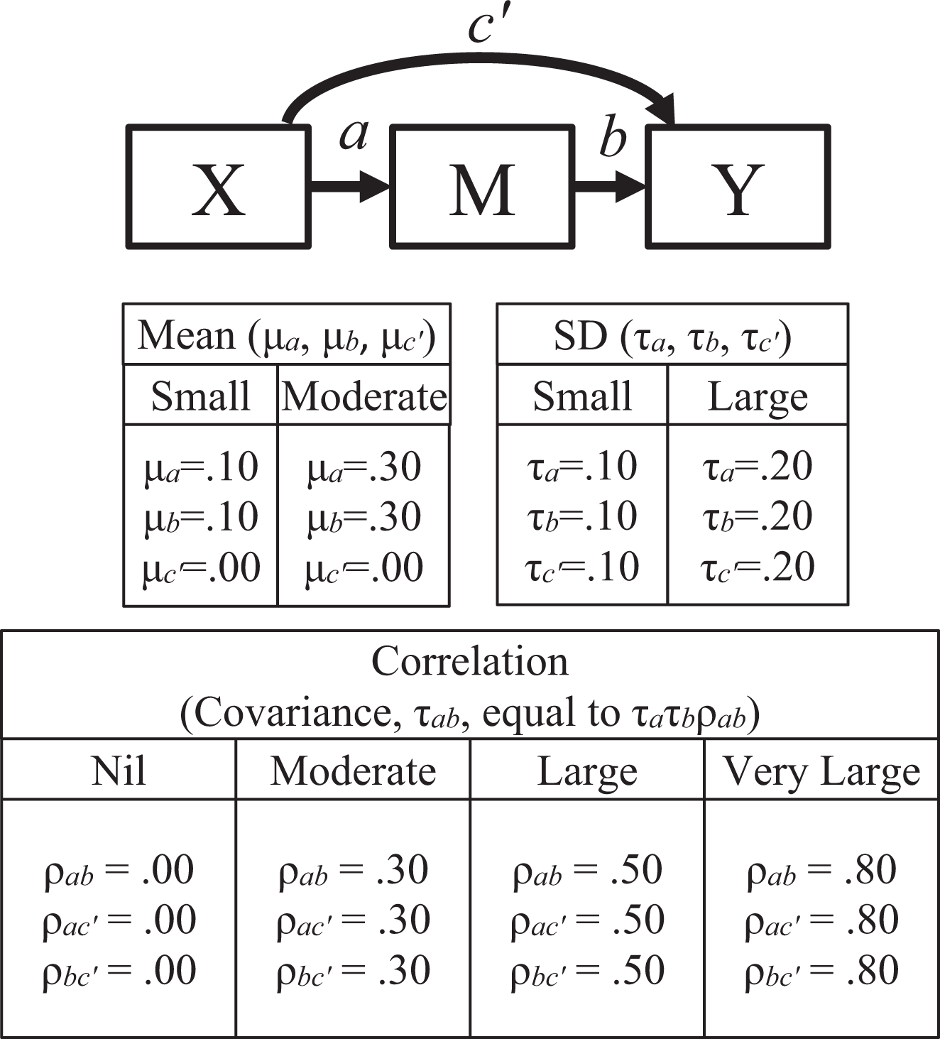
How the model parameters depend on the three factors in the simulation study: Random direct path model.

Data Generation

We generated 10,000 sets of random a, b, and c for each of the 32 combinations of sample sizes, parameter means, random variations, and random covariations. Sets of parameters with at least one of them greater than .95 or implies a nonpositive definite population correlation matrix was replaced by generating another set of parameters. For each set of parameters, n cases of X, M, and Y were generated from a multivariate normal distribution. The sample correlation was then computed, resulting in 10,000 sample correlation matrices for each condition. These sets of population parameters and the implied population correlation matrices were considered the population for the model in corresponding conditions. For each of the two numbers of studies (25 and 50), the target number of sample correlation matrices were randomly selected without replacement, repeated 2,000 times, resulting in 2,000 replications for each condition. The R files of the populations (in RDS format) can be downloaded from Open Science Framework (https://osf.io/zhtrn/?view_only=b56ed3bed7dc4be1b6ebdab09b94a441). In the present study, all studies have no missing correlations.

cMASEM Methods

Stage 1: Estimating mean and random effects of the correlation matrix

We examined three procedures. The first two are based on the SEM-based TSSEM procedure proposed by M. W.-L. Cheung (2014, 2015a) and implemented in the R package metaSEM (version 0.9.12). TSSEM-Diag procedure assumes a diagonal RE model in which correlations have random effect variations but zero random effect covariations. TSSEM-full allows for both random effect variations and covariations. In VOMASEM procedure, one meta-analysis is conducted for each cell in the correlation matrix. Following Yu et al. (2016), we adopted the Hunter-Schmidt procedure (Hunter & Schmidt, 2004; Schmidt & Hunter, 2015) implemented in the metafor R package (Viechtbauer, 2010, version 1.9-9). Similar to TSSEM-Diag, the random effect variation estimates are available in VOMASEM for each cell.

Stage 2: Fitting a path model to the mean correlation matrix

A just-identified partial mediation was fitted in this stage. TSSEM was conducted by the metaSEM package. Following the common practice, in VOMASEM, the mean correlation matrix was submitted to path analysis as if it were a covariance matrix (using the lavaan R package; Rosseel, 2012, version 0.5-23.1097). Without missing data, the total sample size is equal to the harmonic mean and median of sample sizes across cells, two common choices of sample size in Stage 2 of VOMASEM. Therefore, we used the total sample size in path analysis.

Evaluation of the Methods

In the present study, our focus is on estimating the model parameters in the RM. Therefore, we only examined the estimation of model parameter in Stage 2 of cMASEM.

We compared the three procedures on the following criteria: bias, root mean square error (RMSE, equal to the square root of [bias² + standard error²]), the coverage probability of the 95% confidence interval (CI), the Type I error rate in testing the nil mean direct path (c’), and the statistical power in testing the a and b paths.

Results

Bias

As shown in Figure 3, all three procedures had negligible bias across conditions for the three paths (less than .01 for a path and less than .03 for b path and c’ path). As expected from our analytical examination, the bias increased for b path and c’ path as random effect variation and covariation increased. However, even for large random covariation (.80), the bias was still only .03 or less, which is small for a standardized coefficient. As the sample size increased, the already small bias further decreased. The number of studies, on the other hand, had little impact on the bias.

Figure 3.

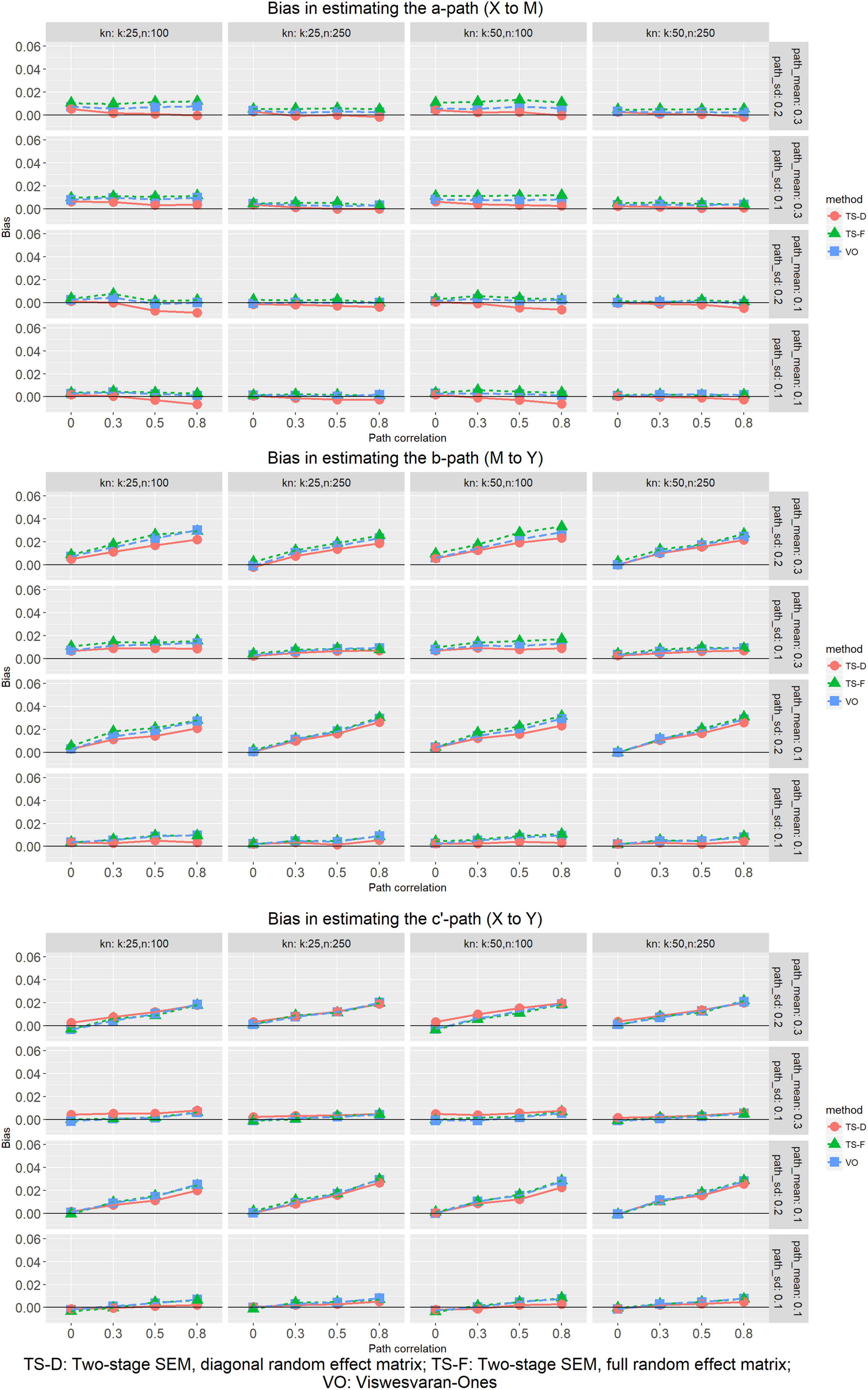
Bias in estimating the path parameter means.

RMSE

As shown in Figure 4, all three procedures yielded virtually the same RMSE in all conditions in estimating the path parameter means. For all three procedures, RMSE decreased when the number of studies increased, the sample size increased, and the random effect variation decreased. As expected from our analytical examination, the RMSE in estimating the b path and the c’ path increased as the random effect covariation increased.

Figure 4.

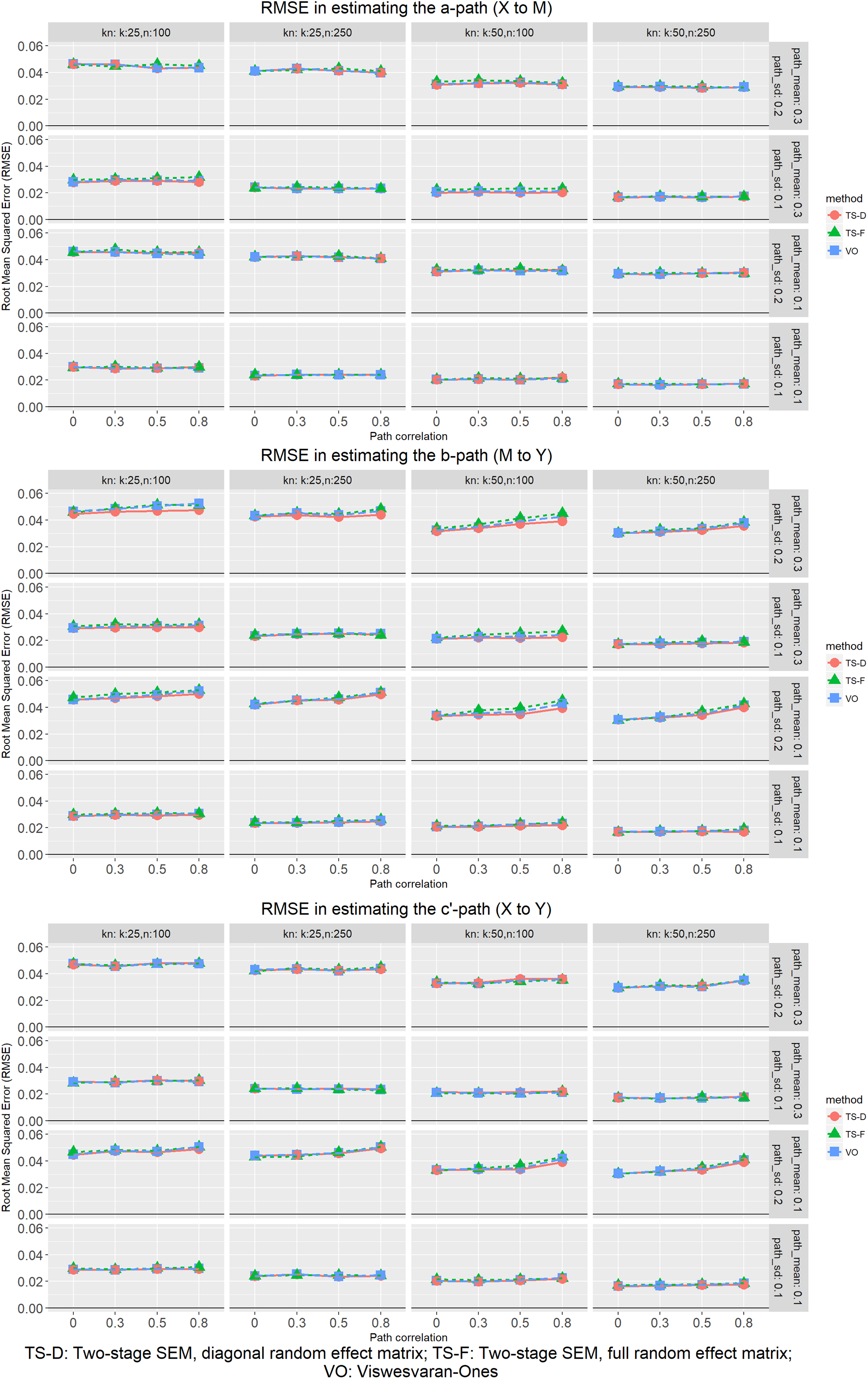
Root mean square error in estimating the path parameter means.

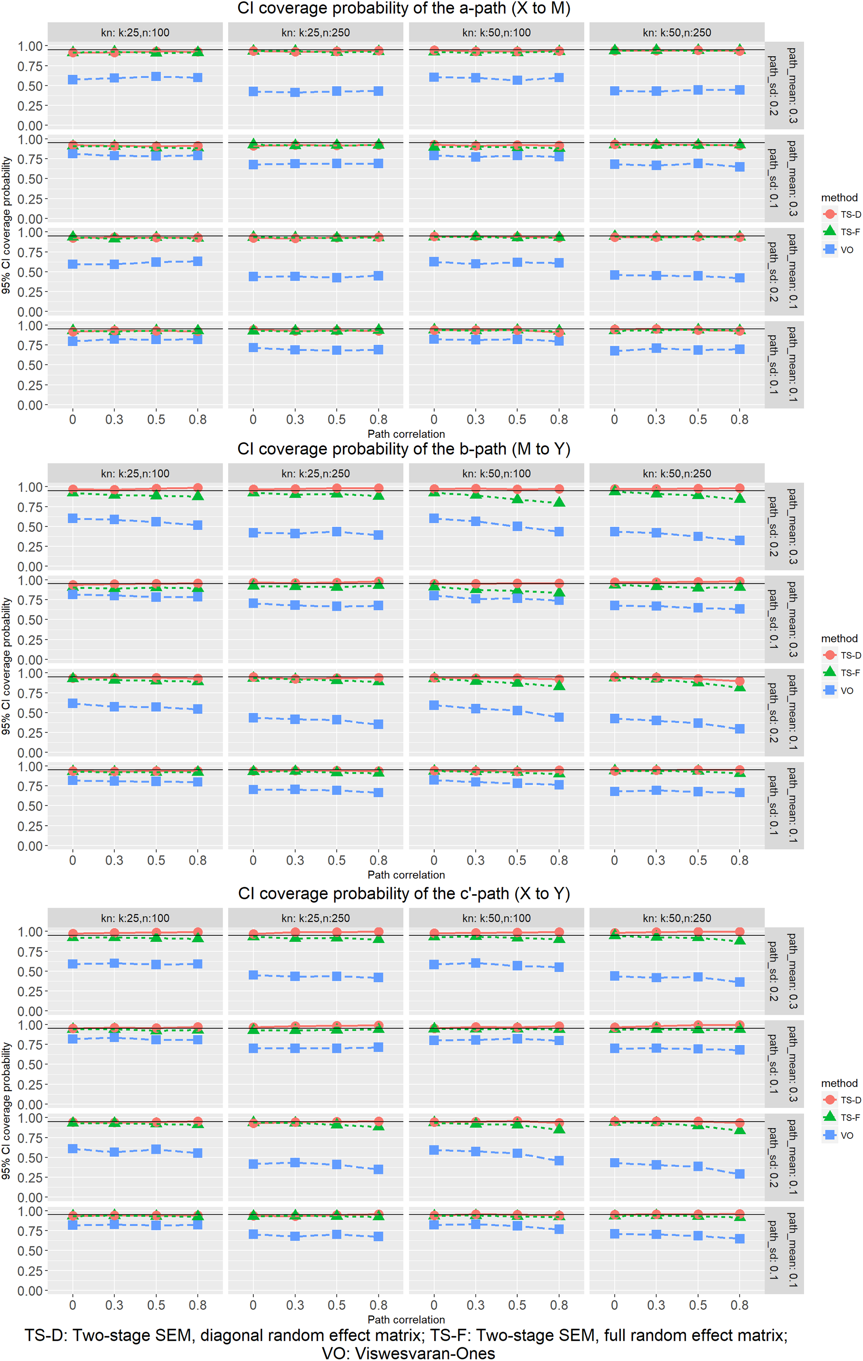
Confidence Interval (95%) Empirical Coverage Probability

Figure 5 shows the empirical coverage probabilities of the 95% CI for the three methods. The coverage probabilities of the two TSSEM procedures were close to the nominal level (95%) in most situations, with one exception. In estimating the b path and the c’ path, if the random effect variation was .20 (in SD) and/or the parameter mean was .30, the TSSEM-full coverage probabilities decreased as random effect covariation increased and the number of studies increased. Nevertheless, the deviation from the nominal level decreased as the sample size increased. Moreover, the deviation from the nominal level was noticeable only when the random effect covariation was unusually large for all parameters.

Figure 5.

Coverage probabilities of the 95% confidence intervals for path parameter means.

The coverage probabilities of VOMASEM, on the other hand, were consistently lower than those of the two TSSEM procedures in all conditions, even in estimating the a path. The VOMASEM coverage probability decreased as the sample size increased, the random effect variation increased, and the random effect covariation increased. One possible explanation is the absence of the estimated random effect in Stage 2 of VOMASEM. The use of the total sample size in Stage 2 of VOMASEM implicitly assumes that variation of the mean correlations from Stage 2 is solely due to sampling variation. Therefore, the larger the random effect, the more the Stage 2 analysis underestimates the sampling variation, resulting in confidence intervals that are narrower than they should be to have the desired level of coverage probabilities. This is analogous to using fixed effect meta-analysis when random effect is present. Because the sampling distributions of the standardized path parameter estimates are not expected to be symmetric, we examined the mean widths of the confidence intervals from the three procedures. As shown in Figure 6, the mean widths of VOMASEM were consistently narrower than those by the TSSEM procedures, supporting our tentative explanation.

Figure 6.

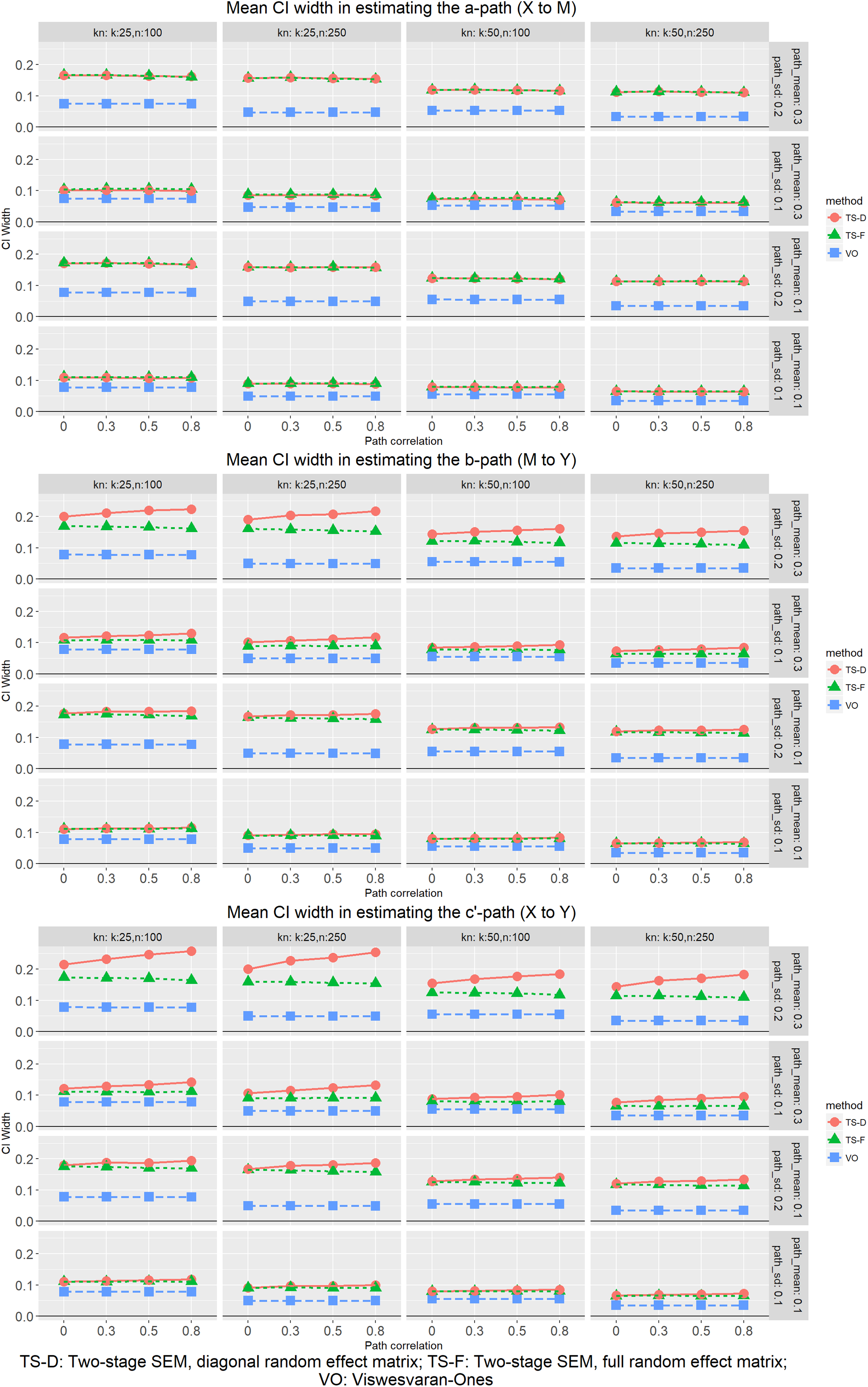
Mean widths of the 95% confidence interval in estimating path parameters.

Note that for the c’ path, which has a population mean of zero, Type I error rate equals to one minus coverage probability (the probability of not including zero). Therefore, the results mentioned previously also mean that the TSSEM procedures had Type I error rates close to the nominal level except that TSSEM-Full showed slight over-rejection when the random effect covariation was large. VOMASEM had inflated Type I error rates in all conditions, and this inflation increased as the sample size increased, the random effect variation increased, and the random effect covariation increased, probably due to not considering Stage 1 random effect estimates as suggested previously.

Power in Testing the a Path and b Path

As shown in Figure 7, VOMASEM had the highest power rate (virtually 100% in nearly all conditions). The TSSEM procedures were similar in power rates, about .80 or higher when the number of studies was 50. With only 25 studies, the power rates of TSSEM procedures could be as low as 60% when parameter means were .10. Because confidence intervals are used in Stage 2 hypothesis testing, the high power of VOMASEM can be explained by its narrower confidence interval compared to TSSEM procedures as discussed previously.

Figure 7.

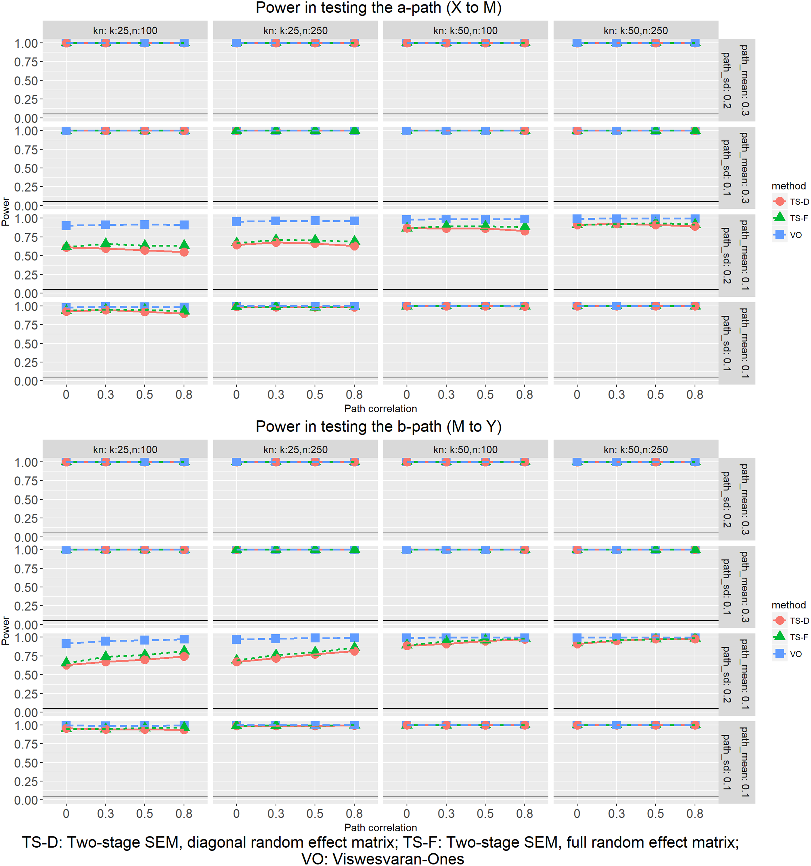
Power in testing the a path (X-M) and the b path (M-Y).

General Discussion and Recommendations

As argued in previous sections, a simulation study is needed because random variation and covariation can result in biases in point estimate, biases in sampling variances (due to biases in estimating random effects), and nonnormal random effects distribution. The performance of a cMASEM procedure is influenced by the joint effect of these three aspects. It is difficult to have simple guidelines or predictions on how random effects variation and covariation can affect the results. Nevertheless, bearing in mind possible exceptions, we would like to propose the following recommendations and reminders based on our results.

First, in point estimation, because random effect covariances in model parameters are bounded by the random effect variances in model parameters, practically the biases in estimating the standardized path coefficients may be of magnitude of .01 or at most .02. Large biases only occur in extreme cases that rarely occurred in realistic situations.

Second, results of the current simulation suggest that confidence intervals from VOMASEM have suboptimal coverage (see Figure 5) in conditions examined. One possible reason is the choice of sample size in Stage 2. Without missing data, it may appear that the total sample size is a natural choice for Stage 2. However, compared to TSSEM, VOMASEM does not consider dependence in the correlations (Yu et al., 2016). As we demonstrated previously, correlations have random effect covariation even if the model parameters vary but are uncorrelated, resulting in larger sampling variation in Stage 2. The results suggest that the total sample size is too large as a proxy to reflect the sampling variation. However, there is no simple way to determine what the appropriate sample size should be, even without missing correlations. TSSEM has been developed exactly to handle this problem by estimating the sampling variance directly. In the current simulation, both TSSEM procedures and the VOMASEM procedure yielded satisfactory or at least acceptable performance in point estimation. The TSSEM procedures yielded superior confidence interval estimation, and the VOMASEM procedure had higher statistical power.

Third, the simulation results suggest that the TSSEM-Diag performed as well as, or better than, TSSEM-Full in the aspects examined. These two procedures had negligible practical differences in bias and RMSE (differences less than .01 for standardized path coefficients), while the confidence interval coverage probabilities of TSSEM-Diag tended to be slightly higher than those of TSSEM-Full. One possible reason for this difference is the number of parameters involved in the full RE model. In Stage 1 of TSSEM, even for three variables, six random effect components are estimated (three variances plus three covariances). Large sample sizes may be required to estimate them accurately. As shown Figure 5, the differences between the two methods decreased as the sample size increased, partly supporting this speculation. Therefore, unless the average sample size was large, the TSSEM-Diag might be preferable to TSSEM-Full. However, more studies are needed to compare TSSEM-Diag and TSSEM-Full in models more complicated than the present one.

Last, in the few conditions in which TSSEM procedures yielded biased estimates or CIs had suboptimal coverage, the problem can increase with the number of studies. This is an important issue in meta-analysis because paradoxically, the more studies we have, the more incorrect the results will become. If researchers suspect that their situations are similar to one of the conditions with large bias or CI suboptimal coverage, the results should be interpreted with caution.

Future Directions

Future research effort is needed to address six issues. First, simulation studies should be conducted to examine to what extent FIMASEM can be used to estimate the random effects in model parameters. In the present study, we focused on estimating the means of model parameters. However, the analysis also suggested that the random effects distribution of the correlations may not be multivariate normal even if the random effects distribution of the model parameter is multivariate normal. Simulation studies are needed to assess how much the assumption of multivariate normality in FIMASEM may affect the estimation of random effects in model parameters. Second, we investigated only conditions with no missing data. We do not expect that the problems found in some conditions will be lessened when there are missing correlations. However, it is possible that the satisfactory performance of a procedure in some conditions may become unsatisfactory in the presence of missing correlations. Third, robust TSSEM may be developed based on current robust methods in SEM to lessen the impact of nonnormal distribution in random effects.¹ Fourth, our analytic discussion and simulation study focus on a simple mediation model. More studies are needed to confirm whether the impact of random effects is also practically minimal in more complicated models. Fifth, further studies can investigate other situations that involve product terms, such as multilevel models with higher level random effect covariations. Last, alternative approaches without the aforementioned problems should be explored. Directly meta-analyzing the sample estimates of the model parameters could be a possible candidate. For example, parameter-based MASEM (M. W.-L. Cheung & Cheung, 2016) avoids all the problems that involve the implied correlation matrix and the average correlation matrix. However, this approach has its own limitations. It requires full correlation matrices from all studies, which is rarely possible in meta-analytic studies. Researchers can explore techniques that allow parameter-based MASEM to handle missing data as TSSEM does.

Supplemental Material

Online_Appendices - Correlation-Based Meta-Analytic Structural Equation Modeling: Effects of Parameter Covariance on Point and Interval Estimates

Online_Appendices for Correlation-Based Meta-Analytic Structural Equation Modeling: Effects of Parameter Covariance on Point and Interval Estimates by Shu Fai Cheung, Rong Wei Sun, and Darius K.-S. Chan in Organizational Research Methods

Footnotes

Declaration of Conflicting Interests

The author(s) declared no potential conflicts of interest with respect to the research, authorship, and/or publication of this article.

Funding

The author(s) disclosed receipt of the following financial support for the research, authorship, and/or publication of this article: This research was supported by the Multi-Year Research Grant (MYRG2016-00068-FSS) from University of Macau.

ORCID iD

Shu Fai Cheung

Supplemental Material

Supplemental material for this article is available online.

Note

References

Ajzen

(1991). The theory of planned behavior. Organizational Behavior and Human Decision Process, 50, 179–211.

Aroian

L. A.

(1947). The probability function of the product of two normally distributed variables. The Annals of Mathematical Statistics, 18, 265–271.

Becker

B. J.

(1992). Using results from replicated studies to estimate linear models. Journal of Educational Statistics, 17, 341–362.

Becker

B. J.

(1995). Corrections to “using results from replicated studies to estimate linear models.” Journal of Educational Statistics, 20, 100–102.

Becker

B. J.

Schram

C. M.

(1994). Examining explanatory models through research synthesis. In Cooper

Hedges

L. V.

(Eds.), The handbook of research synthesis (pp. 357–381). New York, NY: Russell Sage Foundation.

Beus

J. M.

Dhanani

L. Y.

Mccord

M. A.

(2015). A meta-analysis of personality and workplace safety: Addressing unanswered questions. Journal of Applied Psychology, 100, 481–498.

Cheung

M. W.-L.

(2014). Fixed- and random-effects meta-analytic structural equation modeling: Examples and analyses in R. Behavior Research Methods, 46, 29–40.

Cheung

M. W.-L.

(2015a). Meta-analysis: A structural equation modeling approach. Chichester, UK: John Wiley & Sons.

Cheung

M. W.-L.

(2015b). metaSEM: An R package for meta-analysis using structural equation modeling. Frontiers in Psychology, 5, 1521.

10.

Cheung

M. W.-L.

Chan

(2005). Meta-analytic structural equation modeling: A two-stage approach. Psychological Methods, 10, 40–64.

11.

Cheung

M. W.-L.

Cheung

S. F.

(2016). Random-effects models for meta-analytic structural equation modeling: Review, issues, and illustrations. Research Synthesis Methods, 7, 140–155.

12.

Cheung

S. F.

Chan

D. K.-S.

(2000). The role of perceived behavioral control in predicting human behavior: A meta-analytic review of studies on the theory of planned behavior. Unpublished manuscript, Chinese University of Hong Kong.

13.

Colquitt

J. A.

LePine

J. A.

Noe

R. A.

(2000). Toward an integrative theory of training motivation: A meta-analytic path analysis of 20 years of research. Journal of Applied Psychology, 85, 678–707.

14.

Courtright

S. H.

Thurgood

G. R.

Stewart

G. L.

Pierotti

A. J.

(2015). Structural interdependence in teams: An integrative framework and meta-analysis. Journal of Applied Psychology, 100, 1825–1846.

15.

Craig

C. C.

(1936). On the frequency function of xy. The Annals of Mathematical Statistics, 7, 1–15.

16.

Hedges

L. V.

(2016). Applying meta-analysis to structural equation modeling. Research Synthesis Methods, 7, 209–214.

17.

Hedges

L. V.

Vevea

J. L.

(1998). Fixed- and random-effects models in meta-analysis. Psychological Methods, 3, 486–504.

18.

Hong

Liao

Jiang

(2013). Missing link in the service profit chain: A meta-analytic review of the antecedents, consequences, and moderators of service climate. Journal of Applied Psychology, 98, 237–267.

19.

Hunter

J. E.

Schmidt

F. L.

(2004). Methods of meta-analysis: Correcting error and bias in research findings (2nd ed.). Thousand Oaks, CA: Sage Publications.

20.

Joseph

D. L.

Jin

Newman

D. A.

O’Boyle

E. H.

(2015). Why does self-reported emotional intelligence predict job performance? A meta-analytic investigation of mixed EI. Journal of Applied Psychology, 100, 298–342.

21.

Kalaian

H. A.

Raudenbush

S. W.

(1996). A multivariate mixed linear model for meta-analysis. Psychological Methods, 1, 227–235.

22.

Knight

A. P.

Eisenkraft

(2014). Positive is usually good, negative is not always bad: The effects of group affect on social integration and task performance. Journal of Applied Psychology, 100, 1214–1227.

23.

Liu

Huang

J. L.

Wang

(2014). Effectiveness of job search interventions: A meta-analytic review. Psychological Bulletin, 140, 1009–1041.

24.

T. W. H.

Feldman

D. C.

(2015). Ethical leadership: Meta-analytic evidence of criterion-related and incremental validity. Journal of Applied Psychology, 100, 948–965.

25.

Ouellette

J. A.

Wood

(1998). Habit and intention in everyday life: The multiple processes by which past behavior predicts future behavior. Psychological Bulletin, 124, 54–74.

26.

Premack

S. L.

Hunter

J. E.

(1988). Individual unionization decisions. Psychological Bulleting, 103, 223–234.

27.

R Development Core Team. (2017). R: A language and environment for statistical computing. Vienna, Austria: R Foundation for Statistical Computing. Downloaded from https://www.R-project.org/.

28.

Raudenbush

S. W.

Becker

B. J.

Kalaian

(1988). Modeling multivariate effect sizes. Psychological Bulletin, 103, 111–120.

29.

Rosseel

(2012). lavaan: An r package for structural equation modeling. Journal of Statistical Software, 48, 1–36.

30.

Schmidt

F. L.

Hunter

J. E.

(2015). Methods of meta-analysis: Correcting error and bias in research findings (3rd ed.). Thousand Oaks, CA: Sage.

31.

Shadish

W. R.

(1996). Meta-analysis and the exploration of causal mediating processes: A primer of examples, methods, and issues. Psychological Methods, 1, 47–65.

32.

Sheng

Kong

Cortina

J. M.

Hou

(2016). Analyzing matrices of meta-analytic correlations: Current practices and recommendations. Research Synthesis Methods, 7, 187–208.

33.

Tallis

G. M.

(1961). The moment generating function of the truncated multi-normal distribution. Journal of the Royal Statistical Society, Series B (Methodological), 23, 223–229.

34.

Viechtbauer

(2010). Conducting meta-analyses in R with the metafor package. Journal of Statistical Software, 36, 1–48.

35.

Viswesvaran

Ones

D. S.

(1995). Theory testing: Combining psychometric meta-analysis and structural equations modeling. Personnel Psychology, 48, 865–885. doi:10.1111/j.1744-6570.1995.tb01784.x

36.

Viswesvaran

Schmidt

F. L.

Ones

D. S.

(2005). Is there a general factor in ratings of job performance? A meta-analytic framework for disentangling substantive and error influences. Journal of Applied Psychology, 90, 108–131.

37.

World Values Study Group. (1994). World Values Survey, 1981-1984 and 1990-1993 [Computer file]. Ann Arbor, MI: Inter-university Consortium for Political and Social Research.

38.

Downes

P. E.

Carter

K. M.

O’Boyle

E. H.

(2016). The problem of effect size heterogeneity in meta-analytic structural equation modeling. Journal of Applied Psychology, 101, 1457–1473. doi:10.1037/apl0000141

Supplementary Material

Please find the following supplemental material available below.

For Open Access articles published under a Creative Commons License, all supplemental material carries the same license as the article it is associated with.

For non-Open Access articles published, all supplemental material carries a non-exclusive license, and permission requests for re-use of supplemental material or any part of supplemental material shall be sent directly to the copyright owner as specified in the copyright notice associated with the article.

0.00 MB

0.24 MB