




Abstract
Electroencephalography (EEG) was the first of the noninvasive brain measures in neuroscience. Technical advances over the last 100 years or so have rendered EEG a true brain imaging technique. Here, we provide an accessible primer on the biophysics of EEG, on measurement aspects, and on the analysis of EEG data. We use the example of event-related potentials (ERPs), although the issues apply equally to other varieties of EEG signals, and provide an overview of analytic methods at the base of the so-called electrical neuroimaging framework. We detail the interpretational strengths of electrical neuroimaging for organizational researchers and describe some domains of ongoing technical developments. We likewise emphasize practical considerations with the use of EEG in more real-world settings. This primer is intended to provide organizational researchers specifically, and novices more generally, an access point to understanding how EEG may be applied in their research.
Electrophysiological measures date back to the late 19th century and to individuals such as Hermann von Helmholtz, Emil Du Bois-Reymond, Andrew Huxley, Richard Caton, and Hans Berger (Niedermeyer, 2010). Whereas these physiologists were all pioneers in measuring the electrical activity of nerves, Caton was the first to measure the electrical activity of exposed cerebral hemispheres of animals, such as cats, rabbits, and monkeys. Hans Berger is widely recognized as the “discoverer” of human electroencephalography (EEG), after having recorded for the first time human cortical electrical activity at the scalp in the 1920s. Since that time, there have been significant advances along two main axes. On the one hand, the hardware used for data acquisition has allowed for simultaneous recording from hundreds of electrodes distributed over the scalp with sub-millisecond sampling rates (Figure 1). On the other hand, advances in signal processing—certainly itself facilitated by innovations in computer technology—have allowed for more informative inferences regarding the underlying processes (and sometimes mechanisms) giving rise to the signals recorded at the scalp. Advances in signal processing have also allowed for real-time analyses based on continuous activity or single-trial events that are essential for applications in clinics (e.g., brain-computer interfaces) as well as for acquisition in real-world settings critical for applications in organizational research.

EEG electrode montages. EEG montages can range from relatively few (e.g., 16) to several hundred. Here we illustrate the scalp coverage as one progresses from 16 to 32 to 64 to 128 and to 256 electrodes.
Collectively, these advances arguably allow for EEG to be used as a very temporally precise neuroimaging tool (see, e.g., Michel, Koenig, Brandeis, Gianotti, & Wackermann, 2009; Michel & Murray, 2012; Michel, Murray, et al., 2004; Murray, Brunet, & Michel, 2008) that moreover has several major practical strengths (Table 1). Because of the long history of electrophysiologic recordings in nonhuman animals, EEG may more readily allow for translational inference across species. Nevertheless, the exact generation and functional significance of EEG remains a domain of active research and a certain degree of debate, due to issues such as the complexity of the underlying physiology and the level of macro-, meso-, and microscopic levels of description at which the researcher wishes to concentrate (Cohen, 2017; Kajikawa & Schroeder, 2011; Lopes da Silva, 2013; Pesaran et al., 2018). Such issues notwithstanding, EEG (and electrophysiology more broadly) is an exceptionally powerful neuroscientific tool widely used not only in humans, but also across species and contexts from the laboratory to the real world (e.g., Enriquez-Geppert, Huster, & Herrmann, 2017; Matusz, Dikker, Huth, & Perrodin, 2018).
Commonly Reported Strengths and Weaknesses of EEG in Research Settings.
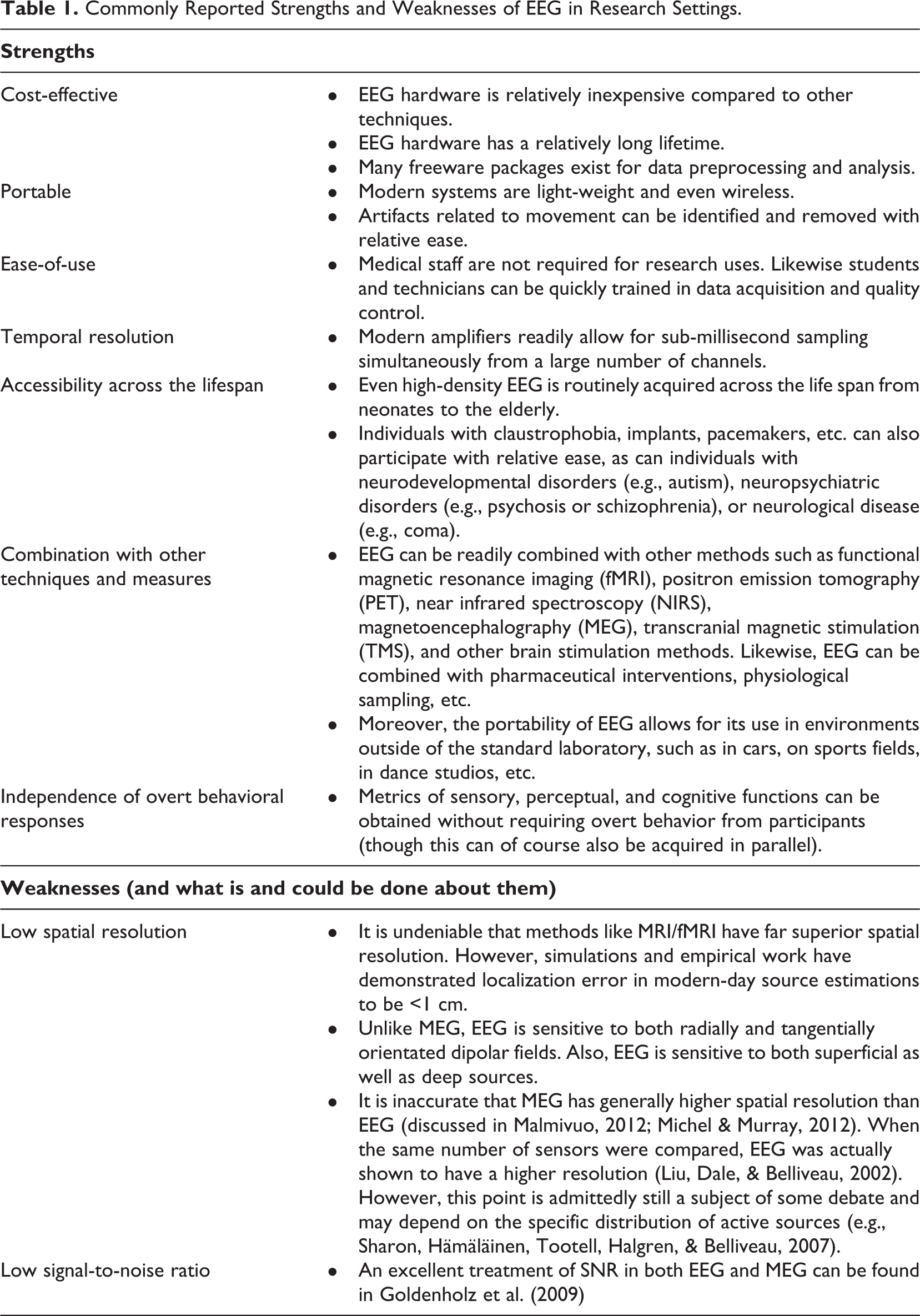
In this primer, we focus on providing organizational researchers with (a) an overview of what EEG measures, (b) some considerations with respect to experimental design and the constraints EEG measures may impose (as well as some opportunities emerging from new analysis techniques), (c) some considerations with regard to dependent measures derived from EEG recordings (with a particular emphasis on the example of event-related potentials [ERPs] for the sake of simplicity and accessibility), and (d) some of the limitations of the EEG method in the context of organizational research. We would encourage motivated readers to consult more extensive reviews and textbooks on specific domains of EEG methods and analysis techniques, which we have done our utmost to highlight throughout this primer.
What EEG Measures
Put simply, EEG measures electrical activity (voltage) related to electrical activity of the brain. As will be detailed below, the electrical activity that EEG can detect is just a portion of all the varieties of electrical activity going on both in the brain and elsewhere. In an effort to use an accessible metaphor, the reader can think of the electrical activity of neurons as comprising both flashes of lighting and its associated thunder. Action potentials are like lightning insofar as they are short lasting and high amplitude electrical pulses. Postsynaptic potentials, which are detailed below, are like thunder insofar as they are longer lasting and of generally lower, though still mixed, amplitude. Although the signal of interest for neuroscientists is the electrical activity of the brain, there are also (unfortunately) other sources of electrical “noise” that often (if not always) are picked up by electrodes on the scalp. These include such things as muscle activity (cardiac, ocular, etc.) as well as nonphysiologic activity (e.g., interference from electrical equipment, power lines, etc.). We return to the topic of EEG data acquisition and analysis below. However, it is foremost germane to describe briefly the kind of brain activity that is, and is not, measured by EEG (we refer readers interested in the biophysics of EEG to Nunez & Srinivasan, 2006).
Neurons are excitable cells with intrinsic electrical properties. 1 They are electrically polarized to about –70 millivolts by the separation of intracellular and extracellular charges, with more negatively charged proteins in the intracellular space. 2 This membrane potential, also called the resting potential of the neuron, is supported by a differential distribution of ions (sodium, potassium, calcium, and chloride). Potassium (K+) and sodium (Na+) influx and efflux, controlled by a sodium-potassium pump, play the main roles in maintaining this resting potential. When a neuron is at this –70 mV resting potential, the sodium channels are shut. When activated, that is when the influx and efflux of ions changes (e.g., sodium channels open in the case of depolarization), neurons produce ionic currents at the level of cellular membranes. In this way, the resting potential of the neuron is disturbed. It is either depolarized (i.e., increased positive polarization due to Na+ influx) or hyperpolarized (i.e., increased negative polarization). A depolarized neuron whose membrane potential is approximately –55 mV will generate action potentials, which are the rapid and orchestrated propagation of current along the length of the neuron’s axon due to these changes in transmembrane potential. Action potentials are suppressed in a hyperpolarized neuron. The current flow associated with an action potential (like any electrical current) also produces electric and magnetic fields around the neuron. However, action potentials are not the main contributor to EEG (e.g., Lopes da Silva, 2013).
Instead, when a neuron generates an action potential it leads to neurotransmitter release at the ends of axons (i.e., at terminal boutons). This neurotransmitter release, which in turn depolarizes or hyperpolarizes the next neuron (i.e., the postsynaptic neuron), results in postsynaptic potentials. Excitatory postsynaptic potentials (EPSPs) result in depolarization of the postsynaptic neuron, whereas inhibitory postsynaptic potentials (IPSPs) result in hyperpolarization of the postsynaptic neuron. These postsynaptic potentials (or more precisely these postsynaptic currents that result in measurable potentials) are all generated at the juncture between the presynaptic neuron that just fired an action potential and the postsynaptic neuron. Let us consider the case of the synaptic cleft being near the apical dendrites of the postsynaptic neuron (i.e., its top). At the site of an EPSP, there is a local current sink generated in the extracellular space (i.e., a negativity) because the adjacent intracellular space is depolarized (i.e., became more positive). In turn, there is effectively a passive current source at the postsynaptic neuron’s soma (i.e., its middle) largely due to the anatomic geometry of pyramidal neurons. This sink-source configuration is referred to as a current dipole, which is essentially like a AA battery (Figure 2). The same occurs in the case of IPSPs, but of opposite polarity (source-sink configuration). These EPSPs and IPSPs are not causally related to whether or not the postsynaptic neuron itself ultimately generates an action potential, because they have to change the membrane potential of the postsynaptic neuron enough to result in its depolarization (discussed in Kajikawa & Schroeder, 2011). More important, these postsynaptic potentials (or more precisely from a biophysics standpoint, postsynaptic currents, though we use the term “postsynaptic potentials” hereafter to remind readers that EEG measures EPSPs and IPSPs rather than action potentials) are the main source of activity measured by EEG. In this regard, it is important to bear in mind that EEG is recording not postsynaptic potentials of individual neurons, but rather local populations of similarly orientated neurons that are essentially simultaneously active. This last aspect—being essentially simultaneously active—is one key contributor to the detectability of this variety of neural signal to the scalp. A second contributing factor is volume conduction of postsynaptic potentials, which recent evidence would suggest is isotropic in cortex, largely independent of the frequency of the signal (even if power follows a “1/f” distribution; He, 2014), and may extend over larger distances than previously thought (Kajikawa & Schroeder, 2011; Logothetis, Kayser, & Oeltermann, 2007). Both of these aspects contribute less in the case of action potentials, which are both short-lived (<1 ms duration) and essentially limited in their volume conduction to the neuronal axon. Any contribution of action potentials to scalp EEG is likely therefore limited.

Biophysics of EEG signal generation. (A) A schematized presynaptic and postsynaptic pyramidal neuron are illustrated. Typically, pyramidal neurons are organized perpendicular to the cortical surface, with dendrites toward the cortical surface and axons pointed toward the gray-white matter border. (B) When the presynaptic neuron results in an excitatory postsynaptic potential (EPSP), here shown at the locus of the apical dendrites, there is a concomitant current source within the intracellular space of the postsynaptic neuron and a current sink in the surrounding extracellular space. Concurrently, there is a passive current at the soma (cell body) of the postsynaptic neuron that results in an intracellular current sink and extracellular current source. (C) This extracellular current sink and current source can be modeled as a current dipole (i.e., a battery). These postsynaptic currents in extracellular space are what is recorded by EEG.
How EEG Is Measured
The basic hardware behind EEG acquisition is straightforward. Electrodes are conductive materials placed on the scalp. 3 Many EEG systems improve the electrode-skin contact, and by extension the quality of recordings, with electrolytic gels or solutions. However, advances are also being made in the use of so-called dry electrode systems that do not require such (Fiedler et al., 2015), and arguably hasten electrode application time and increase accessibility of the technique, including in real-world settings where extensive subject preparation may not always be feasible. In all EEG systems, the electrodes are connected to amplifiers that function to boost the power of a signal (nowadays these are typically digital rather than purely analog). Because digital amplifiers are by definition discontinuous (i.e., they do not measure at each moment in time nor each subunit in strength), they have both a sampling rate in time (measured in hertz) and amplitude resolution (measured in bits). We would encourage newcomers to EEG to consult some of the introductory and highly accessibly books written on laboratory setup and other fundamentals of EEG/MEG (magnetoencephalography; e.g., Hari & Puce, 2017; Luck, 2014). The hardware for acquiring EEG data is relatively straightforward from the engineering standpoint (though continual and consequential improvements are of course still ongoing). Experimenters can choose from a slew of commercially available systems, according to their specific needs and budgets.
The choice of specific hardware notwithstanding, we here first focus on the fact that the measurement of voltage (i.e., potentials) entails the differential measurement between the electrode and a reference site. The need for a reference site is a universal issue in electrophysiology and EEG, but not magnetoencephalography. We then dovetail to the related issue of how many channels the experimenter could and “should” record. This issue is pertinent to both the topic of referential measurements, as well as to the interpretational power of EEG signals and the use of EEG as a brain imaging technique. However, the issue of how many channels is further embroiled in a practical reality imposed by the experimental setup and by an interest in collecting data in as ethologically relevant contexts as possible. Finally, we discuss the types of signals available from multichannel EEG and how to analyze/interpret them, using ERPs as an example.
As detailed above, EEG is primarily measuring postsynaptic potentials of the brain. By definition, voltages refer biophysically to the work needed to move charge between two points without accelerating them. More practically, this means that voltage is the difference between an “active” electrode and the “reference” electrode. By way of analogy, this approach is akin to the geographer’s measurement of altitude relative to sea level. The EEG is simply the measurement of this voltage as a function of time—that is, a time series. A long history of EEG has indeed effectively “stopped” here and considered exclusively the time series quality of the data. At first, this focus was a practical constraint; there were at best a few active electrodes and limited computational methods available. Researchers (and clinicians) would then analyze features of the EEG time series, including frequency spectra and ERPs.
Frequency spectra are obtained by decomposing the time series into a set of sine waves (e.g., via Fourier transformation). 4 Early studies a priori delimited frequency bands and in turn went on to characterize phenomena such as sleep stages or consciousness based on the power distribution of these frequency bands. In such a framework, the EEG can be divided into delta (δ: ∼0.2-3.5 Hz), theta (θ: ∼4-7.5 Hz), alpha (α: ∼8-13 Hz), beta (β: ∼14-30 Hz), gamma (γ: ∼30-90 Hz), and (very) high frequencies (>90 Hz; Lopes da Silva, 2013). One downside has been that a given frequency band was often effectively treated as if it were directly reflective of a specific brain process in a nearly 1:1 manner. Empirical data, in fact, do support these a priori bands being reflective of the structure intrinsic to EEG data (Lopes da Silva, 2013). However, there is also mounting recognition of the contribution of nonsinusoidal signals to analyses based on frequency decompositions, which presume exclusively sinusoidal signals (Gerber, Sadeh, Ward, Knight, & Deouell, 2016; Lozano-Soldevilla, Ter Huurne, & Oostenveld, 2016). Second, increased attention has been given to the presence of irregular, arrhythmic activity, which exhibits scale-free behavior (He, 2014; see also Van de Ville, Britz, & Michel, 2010). A given spectral component might result from either or both synchronized oscillations or arrhythmic activity (He, 2014). Finally, there is also an improved characterization of how activity at one frequency can accelerate or decelerate so as to appear at another frequency (Herrmann, Murray, Ionta, Hutt, & Lefebvre, 2016; Lefebvre, Hutt, Knebel, Whittingstall, & Murray, 2015; Van Zaen et al., 2010; Van Zaen, Murray, Meuli, & Vesin, 2013). All of these observations and characterizations have catalyzed further improvements in EEG signal analysis and our understanding of the biophysics of the brain’s electrical activity, though this is by no means complete yet (Cohen, 2017; Kajikawa & Schroeder, 2011; Lopes da Silva, 2013).
Frequency decompositions of EEG have historically received a great deal of attention, with many hoping that such would help bridge gaps between single-unit recordings and behavior (Buzsáki & Draguhn, 2004). More important for the purposes of this primer, the frequency decompositions can be used to quantify (and distinguish between) both induced brain activity, which is neither phase-locked nor time-locked to a stimulus or other event, as well as evoked brain activity, which is both phase-locked and time-locked (reviewed in Tallon-Baudry & Bertrand, 1999). Oscillations in frequency decompositions can be defined, at any point in time, by their amplitude (µV) and phase (ranging from 0-360° or 0-2π when measured in radians). Given the specific degree of phase-locking of oscillations to stimulus presentation, for example, these can be further decomposed into spontaneous, induced, and evoked activity (Herrmann & Demiralp, 2005). In this framework, spontaneous activity is completely uncorrelated with the occurrence of an experimental condition; induced activity is correlated with experimental conditions, but is not strictly phase-locked to its onset; and evoked activity is strictly phase-locked to stimulus onset. ERPs are the time-locked responses to external (or sometimes internal or even missing) events, such as stimulus presentation (e.g., the presentation of an image or sound; Vaughan, 1969). Typically, ERPs are identified by signal averaging repetitions of the same/similar events in order to increase the signal-to-noise ratio in the time series (see, e.g., Luck, 2014, for an accessible introduction to ERPs, Picton et al., 2000, for a general set of guidelines, or Woodman, 2010, for an introduction to ERPs in studies of attention). However, we would emphasize that event-related activity can be observed reliably in single-trial data of humans (De Lucia, Michel, Clarke, & Murray, 2007; Herrmann, Rach, Vosskuhl, & Strüber, 2014; Tzovara, Murray, Plomp, et al., 2012) as well as nonhuman primates (Shah et al., 2004). As such, ERPs are not a simple phase alignment of spontaneous EEG activity, but also include truly evoked activity (for discussion and empirical data, see Lefebvre et al., 2015; Shah et al., 2004).
However, it is important to return to understanding EEG as the measurement of the electric fields of the brain and, more specifically, to those postsynaptic potentials that are detectable at the scalp surface. For researchers interested in characterizing and understanding brain mechanisms, rather than a neural correlate of a presumed process, then a single time series is insufficient by far to characterize brain activity fully. By the same analogy as above, a geographer cannot characterize a mountain range and its peaks and valleys by only measuring the altitude of a single point. 5 In short, this is the main added value of recording EEG from many channels. However, this is by no means the only one. There are important analytical advantages as well, which we describe next.
How EEG Is Analyzed: From Time Series to Spatial Analyses
The reader should have gleaned at least two facts from the preceding sections. First, EEG is a measurement of voltage, which by definition necessitates the quantification of the difference between an active site and a reference. Second, EEG is a measure of postsynaptic currents that are associated with potentials on the scalp surface. In biophysical terms, the brain and its coverings act as a volume conductor. In practical terms, a given electrode does not solely measure brain activity from immediately beneath it, but rather to a certain degree from the entire brain. These two facts have historically led to (and to some extent continue to result in) gross misuse and misinterpretation of EEG data, regardless of the quality of the experimental design. Using our geographer analogy above, consider how a new terrain is to be charted accurately and in turn navigated safely by others when the map is based on a single measure of amplitude (relative to an arbitrarily defined sea level) that could be situated anywhere in this new terrain.
Here, we use the example of ERPs to illustrate how these above facts about EEG can result in misuse and misinterpretation. We then demonstrate how these pitfalls can be mitigated (if not altogether avoided). Finally, we briefly describe new domains of EEG signal processing pertinent for organizational researchers.
The Reference Problem: From the No-Switzerland Principle to the Swiss Alps Principle
Measurements of voltage are referential. This is an unavoidable truth of electrophysiological recordings. However, the consequences of this reality are not always conveyed or appreciated. For one, users of EEG should realize that there is no perfect reference. There is no electrically neutral spot on the scalp (or body surface for that matter); something that has been referred to as the No-Switzerland Principle (Luck, 2014), likely playing on the notoriety of Switzerland’s neutrality (Table 2). One consequence of the underlying biophysics is that the shape of the EEG time series or ERPs at a given scalp site will change when the reference changes (compare Figures 3A and 3B). This is true for spontaneous data through preprocessed and postprocessed averages. Therefore, the variance around any mean value (e.g., spectral power in the case of frequency decompositions, amplitude in the case of ERPs, etc.) will also change when the reference changes. A further consequence is that the results of statistical contrasts will also change with a changing reference. These consequences can be a major drawback of using EEG and ERPs both in research and in clinical practice. To illustrate why, consider the following gedankenexperiment. A law firm has hired you to use EEG to determine if a patient, who allegedly witnessed a crime in a rehabilitation clinic, exhibits intact memory processes and can give reliable testimony. You record EEG and ERPs while you show the patient initial and repeated presentations of objects as a way to test the integrity of implicit memory. Using one reference you observe a statistically reliable difference (Figure 3A), whereas with another reference you observe none (Figure 3B). Which results are accurate? Analyses of voltage waveforms yields ambiguous results and any inferences are inconclusive. We refer to the consequences of the No-Switzerland Principle as the Iowa Principle (Table 2). The Iowa Principle applies regardless of whether you record from and analyze one electrode (Figure 3) or many electrodes (at least in a mass univariate manner; Figure 4). 6 A related and important issue is the selection of which electrodes and potentially also which periods of time to analyze when data have been collected from more than one electrode. One might be tempted to make this choice based on prior literature, which in principle is a reasonable idea. However, in doing so one should be cognizant of how prior literature may also have been influenced by their choice of the reference, analyzed electrodes, analyzed time periods, and so on. That is, replicating prior “errors” is not forcibly a beneficial endeavor. It should also be pointed out that changing the reference does not simply shift in space the loci (i.e., which electrodes) that exhibit a statistically robust effect (see Figure 1 in Tzovara, Murray, Michel, & De Lucia, 2012). Specifically, the Iowa Principle describes some of the consequences of the fact that voltage waveforms and power spectra are reference-dependent. The data and statistical analyses thereof will therefore change with the choice of the reference (Figure 4). The results of any such analyses will be ambiguous and of limited interpretational value either in terms of the experimental research questions or underlying neurophysiological mechanisms. In these respects, the Iowa Principle can lead to researchers effectively being lost in the middle of nowhere.
Principles of EEG/ERPs.
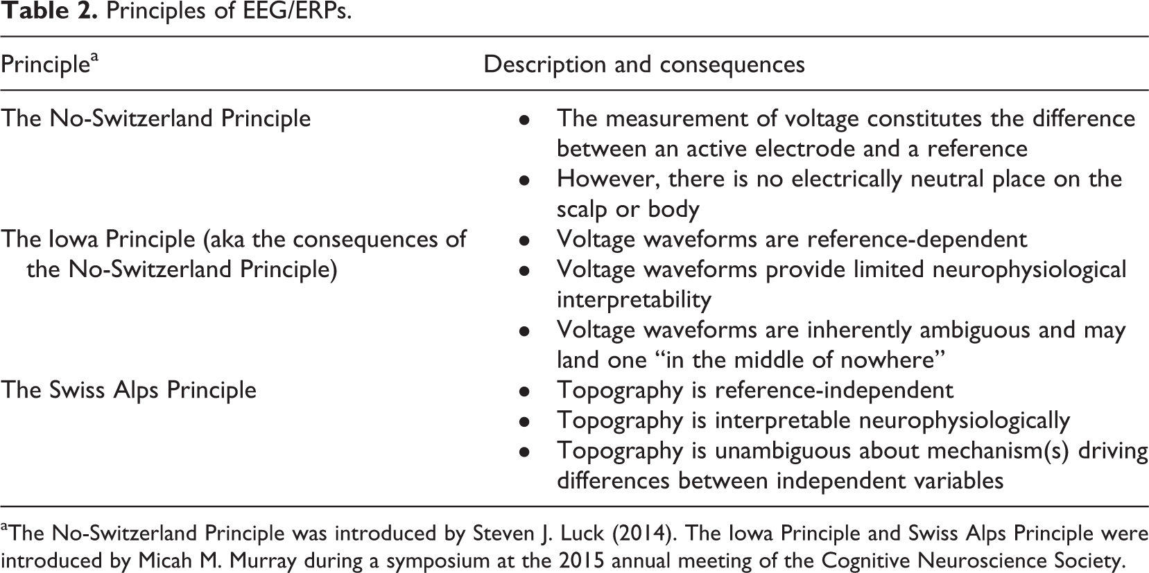
aThe No-Switzerland Principle was introduced by Steven J. Luck (2014). The Iowa Principle and Swiss Alps Principle were introduced by Micah M. Murray during a symposium at the 2015 annual meeting of the Cognitive Neuroscience Society.
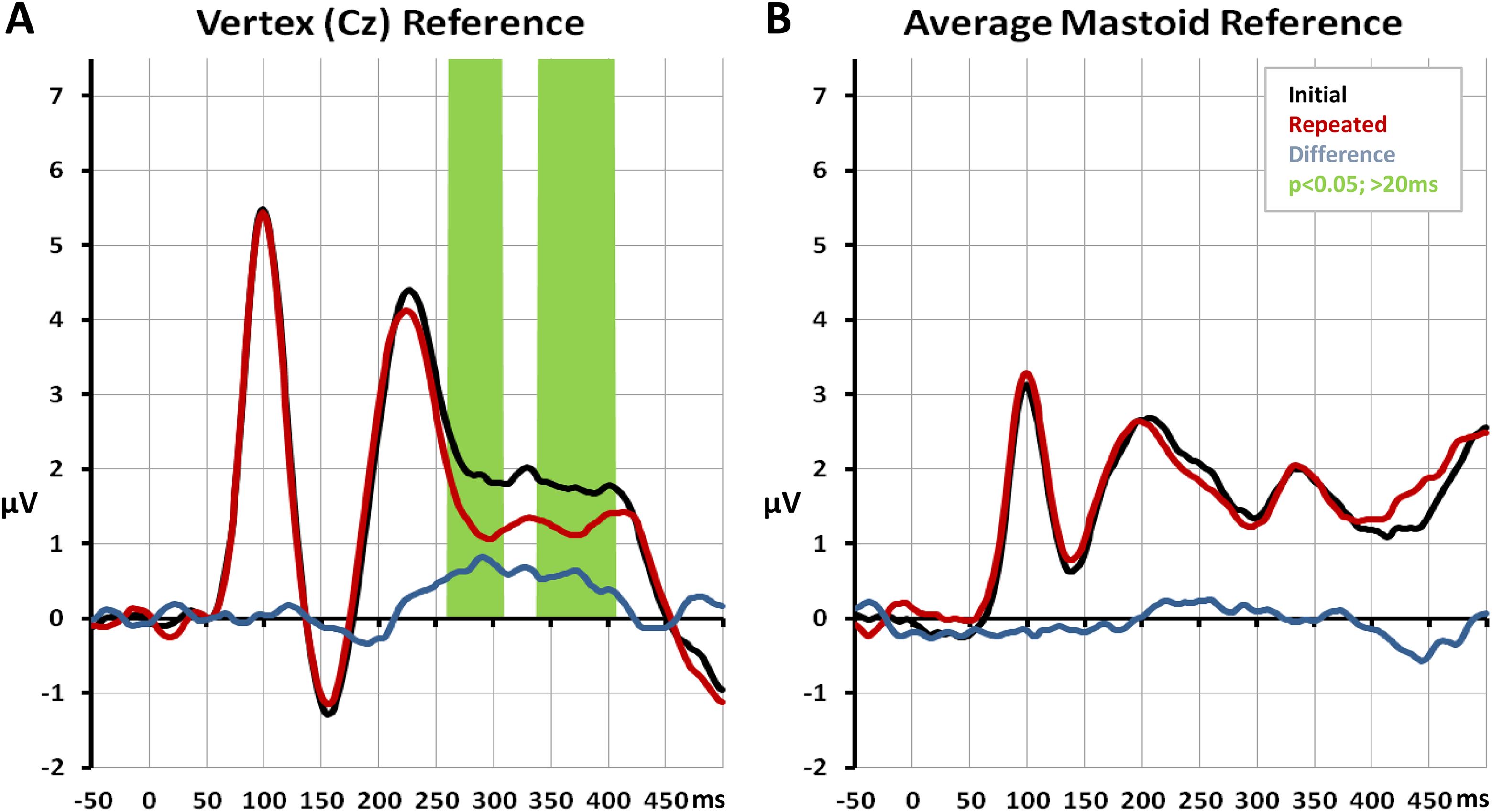
Effects of the reference choice on voltage waveforms and their statistical analysis. The data in panels A and B are identical, except that a vertex reference was used in panel A and an average of the mastoids (loci on the bony protrusion behind each ear) was used in panel B. There is a statistical robust difference observed with one, but not the other, reference choice.

Effects of the reference choice on topographic maps and mass univariate statistical analyses. The data in panels A and B are identical, except that vertex reference was used in panel A and an average of the mastoids was used in panel B. These data are the topographic maps across time poststimulus onset of the same data as in Figure 3, which shows time series from one electrode. The reader should note that whereas the colors ascribed to any point on the topographic map may change as a function of the chosen reference, the shape of the topography (i.e., its peaks and valleys) does not; it is reference independent. The reader should also note that the results of statistical analyses will also change dramatically as a function of the chosen reference.
These consequences of the reference problem may lead some to abandon altogether the use of EEG/ERPs in favor of methods that are not subject to the reference problem (e.g., MEG). Others might opt to ignore the issue and to arbitrarily select a given reference site, perhaps in the hope that all will be “fine” if their colleagues also make the same choice and thus replicate their findings. We would emphasize that this option would in no way resolve the ambiguity issues related to whether or not the findings based on voltage time series indeed truly represent the measured brain processes, nor would one gain insights into the underlying brain mechanisms (i.e., the law firm in the above example would never get an unequivocal response to the mandate they issued to you). Still others instead consider other features of the EEG/ERP that are reference-independent and coincidentally demonstrate the added value of recording from many electrodes. This last tactic is the basis of an analysis framework referred to as electrical neuroimaging (Michel et al., 2009; Michel & Murray, 2012; Murray, De Lucia, Brunet, & Michel, 2009; Murray et al., 2008; Tzovara, Murray, Plomp, et al., 2012).
In order to understand better what we mean by reference-independent, we can return to our geographer analogy. Imagine the abovementioned new terrain. The geographer, whom we will call Alexis, receives a major grant that allows for measuring all of the peaks, valleys, and lakes of the mountain range, based on the notion of sea level defined by the geographer’s government. In this way, Alexis generates a map describing the altitude gradients across this new terrain. At an international conference, Alexis encounters another geographer, Morgan, who has been on a similar mission financed by another government. They discuss their respective maps. However, Alexis soon learns that Morgan’s map has been drawn relative to sky level, which Alexis discovers is the summit of the tallest mountain in Morgan’s homeland. Alexis and Morgan meet to discuss and compare their respective maps. They lay them out on a table side by side. Alexis and Morgan immediately notice that the numbers they each use to characterize various geological formations are not the same. They therefore wonder how to compare their maps. Fortunately, another colleague, Dietrich, points out that the contour lines are the same on both maps and the ground truth of the shape of the terrain remains unchanged, regardless of whether sea level or sky level was used as the reference for altitude. 7 We refer to this fact as the Swiss Alps Principle (Table 2; Figure 4).
What this analogy demonstrates and the Swiss Alps Principle describes is how the shape of the electric field at the scalp—the topography—is independent of the choice of the reference. Whereas this global feature is reference-independent, local features (i.e., numbers ascribed to specific mount peaks in our analogy or voltages at specific electrodes in EEG/ERP data) are entirely reference-dependent. What the reader should also sense is that the description and quantification of the topography (as well as differences between topographies) is helped by higher spatial sampling of the electric field at the scalp—one added value of higher-density electrode montages.
We have emphasized the pitfalls of reference-dependent measures. However, the researcher must nonetheless choose a reference to record and analyze EEG/ERPs. Is this a catch-22 scenario, or is there a “wise” choice to be made? There are several reasons, in our opinion, in favor of using the common average reference, which is the mean across all electrodes at a given moment in time (Lehmann & Skrandies, 1980; Murray et al., 2008). For one, if a researcher’s analysis pipeline includes source estimations (i.e., methods to reconstruct the intracranial sources of surface-recorded data), then the data are by definition recalculated to a common average reference. Source estimation methods are based on the biophysical assumption of quasi-stationarity, which states that the sum of all currents inside the brain at a given moment in time equals zero. This is mathematically identical to the common average reference. Second, the relatively low cost of high-density (i.e., >64 channel) EEG systems allows for researchers to have reasonably good and equidistant coverage of the scalp, making the calculation of the common average reference feasible, including the detection of artifacts as well as preprocessing and “cleaning” of the data. High-density recordings also make the use of global measures of the electric field at the scalp more sensitive. How many electrodes are sufficient and what the optimal distance between electrodes should be are important topics beyond the scope of this primer (discussed in Michel, Murray, et al., 2004; Mumtaz & Malik, 2018; Yao, 2017).
Reference-independent and neurobiologically interpretable measures can be obtained from EEG/ERP data with mathematically simple formulas that we will describe next. However, it is perhaps first worthwhile to recall the kinds of information researchers typically seek to obtain from using EEG. These include distinguishing between modulations in response strength, modulations in the active brain network, changes in the timing/latency of brain processes, or any combination of these mechanisms either at a given moment in time or over a period of time. These types of questions apply both in within-subject designs as well as in between-subject designs (as well as the infinite combinations thereof). Moreover, in the current trend of “big data” and multicenter studies, it is crucial to have easy-to-use ways of homogenizing datasets. Reference-independent, global measures of the electric field at the scalp can fulfill this need (Koenig et al., 2002).
Global Measures of the Electric Field at the Scalp
During the early days of multichannel EEG recordings in the 1970s, pioneers such as Herbert Vaughan Jr. in the Bronx, New York, and Dietrich Lehmann in Zurich, Switzerland (as well as their colleagues) immediately recognized the abovementioned issues related to reference-dependent measures in EEG signal processing. They were already proposing that researchers concentrate on global, topographic measures of the electric field at the scalp (reviewed in Lehmann & Skrandies, 1980, 1984; Vaughan, 1982).
Vaughan Jr. was avant-garde in many respects. Aside from coining the term event-related potential in 1969 (Vaughan, 1969), he was one of the first to concentrate on localization of scalp-recorded brain activity as well as on the neurophysiological mechanisms underlying EEG/ERPs. Vaughan Jr. and his colleagues introduced multicontact depth electrodes into their research with nonhuman primates, which allowed for recording both multiunit activity and local field potentials from all of the cortical laminae simultaneously (reviewed in Schroeder et al., 1995; Vaughan, 1982). This is akin in many regards to the recording of EEG at the scalp from multiple electrodes. Their analyses included the calculation of the current source density (CSD) profile across the contacts, which mathematically is the second spatial derivative or Laplacian of the local field potentials (Nicholson & Freeman, 1975). Vaughan Jr. and his colleagues (as well as some of their contemporaries; e.g., Nunez & Srinivasan, 2006) also applied a similar approach to scalp-recorded data in humans (e.g., Gomes et al., 2001; Murray, Foxe, Higgins, Javitt, & Schroeder, 2001; Saron, Schroeder, Foxe, & Vaughan, 2001). In nontechnical language, the CSD characterizes the topography across the electrodes (it calculates the change in the change of voltage between adjacent electrodes). The CSD provides both a topographic map of current flow perpendicular to the scalp surface, removing current flow parallel to the scalp (i.e., sharpened maps vs. voltage topographies) as well as reference-free time series at electrode positions (e.g., Kayser & Tenke, 2015a; see also a special issue on the topic, discussed in Kayser & Tenke, 2015b).
Lehmann and Skrandies introduced two measures: global field power (GFP) and global dissimilarity (DISS; Lehmann & Skrandies, 1980, 1984). GFP is a measure of response strength. It is calculated as the root mean square of the sum of the squared values from each electrode (vs. the average reference). It represents a version of the reference-free formulation of GFP, which is calculated using the differences between all pairs of electrodes, that has been scaled by the square root of the number of electrodes (Lehmann & Skrandies, 1980, 1984; see also Murray et al., 2008). GFP is always positive and can be analyzed like any other time series. The reader should note, however, that this formula is nonlinear and thus the average GFP is not equal to the GFP of the average. DISS is a measure of how similar or different two topographies are (these can be two maps in time, across conditions, populations, etc.). DISS is calculated as the root mean square of the squared differences between values from each electrode, which have first been scaled by their instantaneous GFP to have the same strength (Lehmann & Skrandies, 1980, 1984; see also Murray et al., 2008). DISS can range in values between 0 and 2, with a value of 0 indicating that the two topographies are identical and with a value of 2 indicating that the two topographies are inverted with respect to each other. DISS is directly related to the Pearson product-moment correlation [C = (2-DISS 2 )/2], which ranges from –1 to 1. DISS can be straightforwardly analyzed with nonparametric randomization tests (Koenig, Kottlow, Stein, & Melie-García, 2011; Kondákor, Pascual-Marqui, Michel, & Lehmann, 1995; Murray et al., 2008). One key interpretational benefit of DISS is that a change in the topography of the electric field at the scalp forcibly indicates there to be a change in the configuration of the underlying intracranial sources (Helmholtz, 1853; Lehmann, 1987; Vaughan, 1982). Thus, these two simple metrics, GFP and DISS, provide the research with reference-independent and orthogonal assessments of response strength and response topography, while also taking full advantage of the entire electrode montage (the researcher need not pick and choose which electrodes to analyze). Since the introduction of GFP and DISS in 1980, additional analysis tools have been developed that characterize and analyze these features (reviewed in Brunet, Murray, & Michel, 2011; Lehmann, 1987; Michel et al., 2009; Michel & Koenig, 2018; Murray et al., 2008; Wackermann, Lehmann, Michel, & Strik, 1993). For example, these tools have led to a fuller understanding of spontaneous EEG and its temporal structure across the life span (Koenig et al., 2002) as well as its scale-free properties (Van de Ville et al., 2010). GFP and DISS have likewise served to better characterize the temporal structure of ERPs, wherein components are defined by their topographic distribution and latency (reviewed in Michel & Murray, 2012; Murray et al., 2008).
Source Localization and Connectivity
As previously emphasized, advances in EEG analysis permit it to be regarded as a brain imaging tool. These advances include the ability to estimate the loci of active sources in the brain based on surface recordings at the scalp. A challenge to this endeavor is the fact that the brain and its coverings act as a volume conductor; sources inside the brain can be detected across the scalp surface to one degree or another. On the one hand, this means that researchers cannot assume that a signal at a given electrode reflects activity emanating from directly beneath it. On the other hand, it results in the solution to the so-called electromagnetic inverse problem being ill-posed and nonunique. This inverse problem refers to determining the intracranial source(s) of the EEG signals measured on the scalp. Solutions to the nonuniqueness of the inverse problem have been formulated through various mathematical formulations, some of which incorporate biophysical constraints (reviewed in Michel & He, 2012; Michel, Murray, et al., 2004). There are two general families of solutions to the inverse problem: equivalent current dipoles and distributed. Equivalent current dipole models a priori specify the number of sources to estimate. Distributed models do not make any assumptions about the number of brain electric sources (Figure 5). Nevertheless and independently of the model used, the solution space must be predefined (e.g., sources can be only in the brain and moreover only in the gray matter). It is likewise important that source estimations are guided by data-driven and theory-driven biophysical assumptions (e.g., Grave De Peralta Menendez, Murray, Michel, Martuzzi, & Gonzalez Andino, 2004). Despite some shortcomings, results from inverse solution modeling have been validated by other neuroimaging and intracranial recordings, and thus offer a reliable estimation of the 3-dimensional distribution of neuronal activity in the whole brain at each moment in time (Michel & He, 2012; Michel & Murray, 2012).

Distributed source estimations allow for modeling of the intracranial currents throughout a matrix of solution points (shown here as blue spheres) that covers the entire brain.
Beyond localizing sources in the brain, researchers are increasingly interested in describing the neural synchrony or communication between different brain areas with functional connectivity measures (Michel & Murray, 2012; Stam & van Straaten, 2012). Connectivity methods permit researchers to see past the surface structure of the EEG, which is usually illustrated in Fourier analysis and ERPs, and into the “deep” structure of brain organization (Fingelkurts, Fingelkurts, & Kähkönen, 2005). The main rationale guiding connectivity analysis is that brain states are arguably characterized by patterns of interactions between specific brain regions (Fingelkurts et al., 2005; Stam & van Straaten, 2012). Functional connectivity describes communication between neural networks, neuroanatomical connectivity describes the likely physiological substrate itself, and effective connectivity is defined as the influence that a neural system exerts over another one (Fingelkurts et al., 2005). Functional connectivity should also be considered alongside other varieties of connectivity, including but not limited to neuroanatomical connectivity and effective connectivity. Connectivity measures will undoubtedly continue to be a major domain of research in the coming years.
EEG in Organizational Research
So where does EEG/ERP find its applications in organizational research? What types of questions could we address, and why should we use EEG recordings to complement classical behavioral studies? As previously stated, EEG is widely used for the study of brain and cognitive states. Perception, attention, motivation, and their neural correlates can all be studied with EEG. If an organizational scholar wishes to understand what neural processes support these states, or how certain influential factors, such as work-related stress or discrimination, can impact them (see, e.g., Becker, Cropanzano, & Sanfey, 2011; Ward, Volk, & Becker, 2015), a neuroscientific approach might be particularly well-suited. When using EEG to investigate a certain brain process, it is important to first ensure that it is the right method to use. In this regard, we encourage the reader to consult the other articles in this special issue for discussions on specific methods and topics. Like every other neuroscientific method, EEG rests on specific physical and physiological assumptions and is subject to certain technological limitations, which are not always completely fulfilled or taken into account (see Tables 1 and 2).
EEG has allowed scientists to look at the real-time unfolding of neural processes, which has helped enormously in the quest to characterize brain mechanisms and cognitive processes (Kappenman & Luck, 2011). One major application of EEG data has been in describing brain states, such as sleep and dreaming (Huber, Ghilardi, Massimini, & Tononi, 2004; Siclari et al., 2017; Tononi & Cirelli, 1999), coma (Fingelkurts, Fingelkurts, Bagnato, Boccagni, & Galardi, 2011; Tzovara et al., 2013), relaxation (Jacobs & Friedman, 2004), or cognitive states, such as focused attention (see, e.g., Woodman, 2010). Moreover, different pathologies have demonstrated specific EEG patterns, such as spike activity during epileptic seizures (Michel, Lantz, et al., 2004), or abnormal EEG/ERPs in schizophrenia (Javitt & Freedman, 2015; Luck et al., 2011) and depression (Fingelkurts et al., 2007).
In order to give an example from organizational research, if one wants to test depression levels in employees within a certain company, one can apply EEG while displaying positive and negative images to their employees. Previous studies show that people with depressive symptoms tend to show an attentional bias to negative stimuli (for a review, see Peckham, McHugh, & Otto, 2010). Therefore, one could then look at the temporal aspects of ERPs induced by positive and negative images in order to ascertain how the activity differs between the two and if some employees show a negative attentional bias.
Brain states can also be described, for example if one wishes to understand how electrical activity is functionally organized during a state of focused attention in the brain. Otherwise, EEG is also used for recording brain activity in experimental conditions, where stimulus-related activity is investigated in corresponding brain regions or across the scalp (Schomer & Lopes da Silva, 2011). Sensory-evoked potentials (visual, somatosensory, auditory, etc.) are elicited by the respective stimuli, and their shape, strength, topography, and location can be statistically analyzed (Michel & Murray, 2012; Murray et al., 2008). When matched to behavior, these results can yield reliable interpretations on the simultaneous activity and processes taking place (including their sequence).
Practical Benefits of EEG in Organizational Research
As this special issue demonstrates, neuroscientific methods in general offer multiple benefits for organizational theory. Reasons such as expanding the research toolbox to complement the subjectivity of self-reports and other behavioral measures, enhancement of our understanding of constructs and their relationships, and new ways to refine theory are some of the quoted benefits that neuroscientific methods can bring to organizational research (Ward et al., 2015). These methods would also allow for a better understanding of the relationship between organizational behavior and our brains (Lindebaum & Zundel, 2013). As with any technique, the danger of overinterpretation or otherwise misconstruing the explanatory power of the data lies not as much with the method as with the researchers themselves (Cropanzano & Becker, 2013). Thus, neuroscientific methods should complement, and not supplant, traditional methods (Becker & Cropanzano, 2010; Buchanan & Bryman, 2009). Such being said, EEG itself as a method offers some practical benefits over other methods, which include its sub-millisecond temporal resolution, its low cost of application, and its good applicability in some clinical and real-world domains (Table 1).
Given its temporal resolution, EEG is method of choice for researchers wanting to assess the temporal organization of cognitive phenomena or brain states. In addition, it is easy to use and requires minimal maintenance and fewer staff to operate as compared to a magnetic resonance imaging (MRI) or MEG system. The cost of undergoing an EEG study is very low compared to that of undergoing other brain imaging/mapping procedures, such as MRI or positron emission tomography (PET). Even high-density EEG (64 electrodes or above) is nowadays cheap and quickly implemented. These methods could be easily adopted by scholars of organizational behavior (Becker et al., 2011). Advancements in technology offer EEG systems that have long lives, with only, for example, some caps or electrode bundles to replace once in a while. Moreover, recent developments have offered extremely quick, uncomplicated, and comfortable methods of using EEG systems.
Organizational Cognition and Underlying Brain Mechanisms
As emphasized above, EEG is a particularly appropriate method to use when temporal dynamics of brain or cognitive processes are the focus of interest. These can vary from processes like attention and perception (brain processes) to decision making, motivation, planning, implicit and explicit attitudes, and analytical reasoning (cognitive processes). Leadership research is one domain that has regularly employed EEG methods (Hannah, Balthazard, Waldman, Jennings, & Thatcher, 2013; Waldman, 2013). For example, emotions and their relationship to leadership have been widely studied in the social sciences (see, e.g., Beatty, 2000; George, 2000; Gooty, Connelly, Griffith, & Gupta, 2010; Humphrey, 2002; Madera & Smith, 2009; Prati, Douglas, Ferris, Ammeter, & Buckley, 2003). Theories regarding the possible relationships between emotions and leadership have been formulated, and some researchers have investigated how emotional balance could be related to leadership (Waldman, Balthazard, & Peterson, 2011). Furthermore, combined with neuroscientific observations, such as the observation of dysfunctions in the neural processing within frontal brain regions in antisocial behavioral disorders, and the association of frontal regions with social and emotional skills (Waldman et al., 2011), the authors hypothesized that successful leaders should be associated with better emotional functioning, and thus with better frontal functioning. They further hypothesized that this should find expression in patterns of increased connectivity—or communication—between frontal brain regions. Leader self-complexity has also been studied with EEG measures (Hannah et al., 2013), and correlated with adaptive decision making. The authors observed that EEG data and psychological self-reports explained a high amount of variance in an adaptive decision-making task. Other examples of applications of EEG in organizational research include studies of teamwork (Stevens, Galloway, Wang, & Berka, 2012) and conflict (Ward et al., 2015), ergonomics and sleep effects on work performance (see, e.g., Mitler, Miller, Lipsitz, Walsh, & Wylie, 1997; Torsvall & Åkerstedt, 1987), as well as distinctions in top performers (Waldman et al., 2013).
Individual differences can also be investigated with EEG methods. Goal-directed interventions can also be informed by EEG results. From simple feedback to neurofeedback and training, and all the way to clinical interventions, EEG results can be employed for developmental purposes, such as training some of the brain’s functions (Enriquez-Geppert et al., 2017). This then allows the brain to regulate itself and function better, for example by better regulating the intensity of stress reactions (reviewed in Waldman et al., 2011). Although even simple feedback techniques have proved very useful when properly employed (for a review, see Kluger & DeNisi, 1996), neurofeedback techniques may offer a promising brain workout.
Limitations and Considerations
We would hasten to note several, nonexhaustive limitations and considerations when applying neuroscientific methods in general to the study of organizational behavior. One limitation concerns the scientific reductionism that neuroscientific methods typically entail (if not require; Becker et al., 2011; Edwards, 2013; Healey & Hodgkinson, 2014; Lindebaum & Zundel, 2013; Ward et al., 2011, p. 13). One cannot readily reduce complex processes and behavior (e.g., leadership, charisma, etc.) to electrochemical activity in the brain. Some authors underscore the importance of context in organizational neuroscience (see, e.g., Healey & Hodgkinson, 2014; Rousseau & Fried, 2001), pointing out that not all influences on performance lie within the individual. However, the problem of reductionism has itself been debated (see, e.g., Bickle, 2012), and current reductionism tendencies are being steered toward more holistic interpretations, as is visible, for example, in the transition from modular brain region analysis toward functional connectivity analysis across the spectrum of brain imaging and mapping techniques. However, it is still important that the results of neuroscientific methods are not being sensationalized either by scientists or the media.
A second consideration is causality (see, e.g., Antonakis, Bendahan, Jacquart, & Lalive, 2010). It is difficult to infer causal relationships between behavior and neural activation. This problem of reverse inference has been observed by organizational theorists (see, e.g., Lee, Senior, & Butler, 2012; Nicolaou & Shane, 2014), who have pointed out that it is impossible to directly infer complex social behavior from brain activation (Lee et al., 2012; Lindebaum & Zundel, 2013) due to the multiple realization problem (Putnam, 1967). This problem states that a diverse combination of neural processes can manifest in the same psychological state (Bickle, 2010). Moreover, when multiple brain regions are measured, some of these regions might activate by chance due to the experimental manipulation. Thus, scholars are cautioned against trying to pinpoint the roots of behavior in neural activation (Lindebaum & Zundel, 2013).
Another issue that has been raised by organizational theorists is the reverse side of using neuroscientific results to optimize behavior (Cropanzano & Becker, 2013), that is, the phenomenon of “pathologizing” healthy but less effective leaders due to insufficient performance (Lindebaum, 2013, 2016; Waldman et al., 2011). Scholars are thus urged to use caution in their interpretation of neuroscientific results and in the application of intervention techniques based on such results. This limitation should not discourage the use of such techniques to develop specific skills, as they have a huge potential of influencing the malleability of knowledge and abilities (Mishra, Anguera, & Gazzaley, 2016; Ward et al., 2011, p. 34). Nevertheless, these techniques are imperfect, and results are valid only if one follows a thorough method. In addition, and again as this special issue demonstrates, it is important for researchers to understand not only the physiological underpinnings of the signals measured with a given neuroscientific technique, but also the technique’s analytical and interpretational assumptions and constraints (e.g., the issue of neurovascular coupling in fMRI; Cropanzano & Becker, 2013). However, these issues do not suggest that these methods should not be used. Neuroscience has proven a very powerful and reliable tool for the investigation of brain processes, bringing invaluable information for the study of both healthy and pathological brain and cognitive states.
A fourth important issue with using neuroscientific methods is the real-world ethological validity of laboratory experiments (e.g., Matusz et al., 2018; Senior & Lee, 2013; Ward et al., 2011, p. 33). When response tendencies are identified in laboratory settings, they might not translate to behavior in real-world situations. These tendencies might be suppressed by other situational factors or behaviors, and thus, further research in these contextual variables is also needed (Ward et al., 2011, p. 33). This artificiality of laboratory results has also been a long-standing issue in the fields of organizational psychology and neuroscience itself (see, e.g., Dipboye & Flanagan, 1979; Spooner & Pachana, 2006); thus, this limitation is about the generalizability of laboratory experiments per se. However, many commentators, in psychology and in organizational sciences, do not see this issue as major, and there is much more concordance between laboratory and field findings than some sceptics may assume (Anderson, Lindsay, & Bushman, 1999). Nevertheless, the gains of being able to isolate a phenomenon from influencing factors, and study it in such isolation, have often proven greater than the cost of transferring knowledge from the laboratory to real-world settings. In addition, measuring objective biological indicators is less prone to biases as compared to measuring perceptions and using cross-sectional surveys, as is often done in organizational sciences (Antonakis, 2017). As Nicolaou and Shane (2013) recommend, one should view these techniques neither as perfect nor as fundamentally flawed.
Conclusions and Outlook
To conclude, neuroscientific methods, and specifically—EEG, have important explanatory contributions to add to concepts of organizational behavior. Moreover, findings on the neural bases of organizational behavior could inform neuroscience in return (Healey & Hodgkinson, 2014). Linking organizational behavior to cortical functioning in a truly interdisciplinary manner (Waldman, 2013) will surely shed further light on such behavior, which, in turn, can inform managerial and even clinical interventions. As we have tried to detail in this primer, EEG is a particularly powerful neuroscientific method. However, like any method it must be understood in terms of its physiological bases, and also in terms of the issues pertaining to signal processing. EEG neither reads minds nor is it a worthless pseudo-phrenological activity (Logothetis, 2008). This primer sought to motivate organizational scholars to have a fuller understanding of EEG and its potential use in their research, highlighting analytical and interpretational issues that nowadays can be readily circumvented. It is argued that only in this way can we properly use tools such as EEG, and thus obtain valid and reliable results.
Footnotes
Declaration of Conflicting Interests
The author(s) declared no potential conflicts of interest with respect to the research, authorship, and/or publication of this article.
Funding
The author(s) disclosed receipt of the following financial support for the research, authorship, and/or publication of this article: Financial support has been provided by the Swiss National Science Foundation (320030-149982, 320030-169206, and 51NF40-158776), by the Foundation Asile des Aveugles, and by a grantor advised by Carigest SA.
