



Abstract
Recent developments in theories and data collection methods have made intensive longitudinal data (ILD) increasingly relevant and available for organizational research. New methods for analyzing ILD have emerged under the multilevel modeling framework. In this article, we first delineate features of ILD (including autoregressive relationships, trends, cycles/seasons, and between-subject variability in temporal trends). We discuss the analytic challenges for handling ILD using traditional analytic tools familiar to organizational researchers (e.g., growth models, single-subject time series analyses). We then introduce a statistical approach for handling ILD from the multilevel modeling framework: dynamic structural equation modeling (DSEM). We provide three examples using simulated data sets to demonstrate how to apply DSEM to examine ILD with a software program familiar to organizational researchers (i.e., Mplus). Finally, we discuss issues related to applying DSEM, including centering, missing data, and sample size.
Keywords
Data sets with a long series of repeated measurements from the same subjects, namely, intensive longitudinal data (ILD), are increasingly relevant and available to organizational research. Developments in both theories and methodology have propelled this emerging trend of working with ILD. On the one hand, theories about individuals, teams, and organizations are paying more attention to the role of time and process-oriented mechanisms (Cronin & Vancouver, 2019; Kozlowski, Chao, Grand, Braun, & Kuljanin, 2013; Wang, Zhou, & Zhang, 2016). For example, research of individual workers’ motivations, behaviors, attitudes, and well-being have advanced to studying within-person changes over time as well as the between-person differences in the trajectories of changes (e.g., Beal, Weiss, Barros, & MacDermid, 2005; Fuller et al., 2003; Gabriel & Diefendorff, 2015). In work groups and teams research, researchers are starting to unpack the emergence process driven by a series of interactions among team members (e.g., Grand, Braun, Kuljanin, Kozlowski, & Chao, 2016). In addition, theories of firm-level relationships have also incorporated time to explicate the interaction between organizations and their external environment (e.g., Kim & Ployhart, 2014). Moreover, a stream of research is particularly concerned about process-oriented mechanisms that underlie observed changes, such as self-regulation processes in individual and team goal pursuits (e.g., Vancouver, Weinhardt, & Schmidt, 2010; Zhou, Wang, & Vancouver, in press), emergence processes in teams (e.g., Grand et al., 2016), and the emergence of human capital resources in firms (e.g., Ployhart & Moliterno, 2011). These more complicated theories need to be tested by longitudinal studies that provide more fine-grained observations of the phenomena over time (Wang et al., 2016).
On the other hand, new technologies and data collection methods have enabled organizational researchers to access data—either through primary data collection or archival data analyses—that include more extended series of observations from the same subjects. A few developments on this front are worth noting. First, experience sampling method (ESM) has guided studies that collect repeated measurements from the same individuals and teams over the course of multiple days, weeks, or even months (Beal, 2015; Song, Liu, Shi, & Wang, 2017; Zhou, Song, Alterman, Liu, & Wang, 2019). With new devices that allow high-frequency, undisrupted data collection and transmission (e.g., wearable fitness trackers), high-frequency assessment methods allow researchers to obtain more intensive measurements than traditional ESM (Gabriel, Diefendorff, Bennett, & Sloan, 2016). In addition, teams researchers have been interested in using wearable sensors to help document more detailed information about team members’ movements and communications (Chaffin et al., 2015).
As for secondary analyses using archival data, new information and communication technologies have boosted the volume of raw data and the type of data available for organizational research (Barnes, Dang, Leavitt, Guarana, & Uhlmann, 2015). For example, organizations have an ever increasing volume of digitalized information about the organizations as collectives (e.g., firm performance) as well as employees and organizational units (e.g., compensation records, customer satisfaction ratings, and email traces). The online presence of individual workers and firms also provides an enormous amount of content and interactions generated by users (e.g., customer reviews on Yelp, social networks among job seekers on LinkedIn). However, organizational researchers should be aware that these newer forms of primary data (e.g., data collected by wearable fitness trackers) or archival data (e.g., Tweets and Facebook comments) are very likely to have a much lower signal-to-noise ratio in the raw data than conventional design-driven data (e.g., primary field survey data or census data). Thus, great care should be taken to validate the measurements derived from these newer forms of raw data. The statistical methods we will describe later should only be applied to measurements derived from raw data that have acceptable psychometric properties.
The needs for testing complex theories and the new opportunities for data accruement call for new statistical methods; otherwise, theories may not be properly tested and new data opportunities can be missed. By collapsing across measurements or using qualitative descriptions of temporal patterns, existing studies may have overlooked interesting nuances in their ILD that can provide important theoretical insights. To move beyond forcing ILD into lower-frequency data, we need to overcome challenges posed by ILD to traditional analytic methods familiar to organizational researchers (e.g., growth models, single-subject time series analysis). However, there has been limited discussions about statistical methods for ILD, especially in micro and meso organizational research. For example, in one of the leading research methods journals, Organizational Research Methods, only a limited number of articles have been devoted to methods for ILD (e.g., Dass & Shropshire, 2012; Jebb & Tay, 2017). Moreover, these articles mostly focused on explaining the basic concepts of longitudinal data analyses with limited discussions about the issues specific to formally modeling ILD. In particular, Jebb and Tay (2017) focused on exploratory data analyses techniques, and the method introduced in Dass and Shropshire (2012) uses continuous smooth curves created from observed data as the basic analysis units. Considering that most organizational researchers would be interested in a tool that allows testing a priori hypotheses in a sample of subjects (i.e., N > 1), we believe that a statistical method for ILD built from a multilevel modeling framework can be particularly valuable to organizational researchers.
In the rest of this article, we first describe features of ILD and challenges for analyzing ILD. We also provide an overview of statistical models and concepts that serve as the foundation for multilevel models for ILD. We then introduce one of the most promising approaches for specifying and estimating multilevel models for ILD: dynamic structural equation modeling (DSEM). We will also provide demonstrations of DSEM using the software Mplus (L. K. Muthén & Muthén, 2017), which is already familiar to many organizational researchers. When describing these modeling techniques, we assume users already know what effects are to be tested a priori (i.e., theory-driven model testing). Tools for exploratory analyses of time series using graphs or other methods (e.g., periodogram) are explained in Jebb and Tay (2017).
What Are Intensive Longitudinal Data and the Challenges for Analyzing ILD?
A few key terms will be used throughout this article. First, longitudinal designs are often categorized into two types (Collins, 2006): longitudinal panel design, where there are relatively fewer measurements separated by longer intervals (e.g., four measurements of newcomer role clarity separated by one month in between), and intensive longitudinal design, where there are at least 15 to 20 measurements and the time interval between measurements is much shorter (e.g., 96 measurements of mood once every 15 min). This article focuses on data collected from the intensive longitudinal design. Traditionally, in studies using longitudinal panel design, the number of subjects is almost always larger than the number of measurements, whereas in studies using intensive longitudinal design, the number of subjects can be one or a few, much smaller than the number of measurements. However, it should be noted that some longitudinal research falls somewhere in between and may be able to utilize a variety of designs and analytic methods. In addition, in ILD, the number of subjects does not necessarily need to be smaller than the number of measurements. Second, we use subject to refer to study units from which repeated measurements are taken, such as individuals whose emotional states are captured over time or firms whose performance levels are measured over time. Thus, we use the term ILD to refer to a data set including a large volume of within-subject observations from a sample of multiple subjects.
Features of Intensive Longitudinal Data
ILD from a single subject can include one or more basic features of time series: autocorrelations, trends, and cycles (Jebb & Tay, 2017). First, time series are characterized by correlations between observations at adjacent measurements, which is called autoregressive relationship, autocorrelation structure, serial dependency, or lagged relationship with the variable itself (Box, Jenkins, Reinsel, & Ljung, 2016; Hamaker, Asparouhov, Brose, Schmiedek, & Muthén, 2018; Schafer & Walls, 2006; Shumway & Stoffer, 2017). For example, in Figure 1, the amount of drinking at a later time tends to follow the amount of drinking occurring immediately before. The levels of an individual’s or a firm’s performance at adjacent moments (e.g., between 2 days or 2 weeks) are correlated with each other. Second, trends are changes in the absolute level of a variable in a given time window. For example, as illustrated in Figure 1, participant A’s drinking shows a weak negative trend from the beginning to the end of the study. Trends are widely studied in organizational research, and growth models are often used to represent theories about trends (e.g., Judge, Klinger, & Simon, 2010; Wang, 2007). Third, there can be cycles and seasons in ILD. As illustrated in Figure 1, both time series from participants A and B go up and down about once every five measurements. Assuming these measurements are from every Monday to Friday, this cyclic pattern may reflect changes in work-related stressors over the course of a week. We use cycle to refer to the number of measurements that a stable cyclical pattern takes to repeat itself once and frequency to refer to the number of cycles per measurement (i.e., frequency = 1/cycle; Shumway & Stoffer, 2017). Seasons and cycles differ depending on whether the length of each repeated pattern is fixed or not (Jebb & Tay, 2017). In this article, we do not differentiate these two terms in order not to overcomplicate our discussion.

Time series from individual subjects.
In addition to these features in any single time series, a set of time series that forms an ILD also includes between-subject differences in these within-subject temporal features. For example, in Figure 1, in comparison to participant A’s time series, participant B’s drinking stays the same at the end versus at the beginning of the study. Furthermore, within one set of ILD, some subjects can be nested in the same higher-level units. For example, participants in a drinking study can be nested in dyads (e.g., mentor-protégé, husband-wife) or teams (e.g., teammates serving the same client). In summary, variability in an entire set of ILD (e.g., variances in drinking behavior) reflects the combined effects of within-subject differences (e.g., time-varying emotional states), between-subject differences (e.g., personality traits), and between-group differences (e.g., a couple’s marriage quality, group climate).
Note that even when these temporal features exist in the population of interest and a theory clearly identifies these components, whether an ILD set from a particular sample shows these features can be influenced by the design used in data collection, including duration of the study, schedule of measurements, and time interval between measurements (or measurement frequency). For example, assuming that data generation is driven by a slow growth and a strong serial dependent process, when the study duration is too short, the data may not capture the growth trend and once the autoregressive relationship is accounted for in the analyses, trend parameter would not be meaningful anymore. It is also possible that a panel design is used where measurements are not close enough to each other and misses important information about the internal dynamics of a system (e.g., stability, inertia, and self-regulation). Other possible scenarios include that the study period is too short to allow a full cycle to finish or a large interval together with a fixed schedule is used that systematically misses certain parts of the cycles (e.g., a total of five measurements on five Mondays when the system goes through a cycle every Monday to Friday). Considering these issues, it is important to identify the “optimal” design elements before data collection by drawing on prior theories, methodology literature, and existing empirical studies (if properly designed); discussion with subject matter experts; and conducting pilot studies (Dormann & Griffin, 2015; Ployhart & Vandenberg, 2010).
Another important issue is that although ILD is composed of multiple time series, not all statistical procedures for single-subject time series directly apply to ILD, especially when ILD includes more than just autoregressive relationships. A key concept in traditional single-subject time series analysis is stationarity. As defined in Shumway and Stoffer (2017), “a strictly stationary time series is one for which the probabilistic behavior of every collection of values {
An Example and Simulated Data
We use employee drinking behavior as a running example throughout this article. Prior research has shown drinking behavior has both within-person and between-person variations, and it is associated with both work and nonwork factors (e.g., S. Liu, Wang, Bamberger, Shi, & Bacharach, 2015; S. Liu, Wang, Zhan, & Shi, 2009; Wang, Liu, Zhan, & Shi, 2010). In our example, a researcher who studies employee drinking follows a group of 200 participants for 21 weeks. The amount of drinking after work hours and the urge to drink experienced at work (simply called urge in the rest of this article) are measured once each workday (i.e., Monday to Friday, excluding weekends), which yields a total of 105 measurements per participant. The researcher also measures individual differences (including age, gender, neuroticism, organizational drinking norm) prior to daily measurements and outcomes (including weight, job performance, and overall psychological well-being) at the end of the study. In general, the researcher is interested in (a) whether previous day’s drinking is related to next day’s drinking (i.e., an autoregressive relationship); (b) whether drinking after work hours and drinking urge felt at work on the next day are related to each other (i.e., cross-lagged relationships); (c) whether the magnitude of within-person fluctuation in drinking is consistent across individuals; (d) whether individual differences are associated with the average level of drinking, magnitudes of autoregressive relationships, the magnitudes of cross-lagged relationships; and (e) whether the average level of drinking, magnitudes of autoregressive relationships, and magnitudes of cross-lagged relationships are related to more distal outcomes. In addition, although the researcher does not have a priori hypotheses about the fluctuation in drinking from week to week, he or she knows that the job requirements of the participants tend to vary by cycles. Thus, the research wants to examine weekly cycles of drinking in supplemental analyses.
We simulated a data set for this example. Data simulation was conducted in software Mplus 8.2, and codes are available in Appendix A in the online version of the journal (Dataset 1; readers can also contact the first author for the simulated data sets). This data set included four variables, two with 105 repeated measurements and two subject-level variables. A total of 200 subjects were simulated. Data collected in studies with a similar design as our example can be organized following a general template illustrated in Table 1. In longitudinal analyses, structuring the data this way is also called using the long format or stacked format. It should be noted that although we use this example of repeated measurements nested in individuals for illustrative purpose, the techniques introduced here can also be applied to studying repeated observations from organizations over time.
An Illustration of an Intensive Longitudinal Data Set.

Note: N = number of subjects; T = number of measurements per subject; W and Z are subject-level variables; Y and X are measurement-level variables.
Analytic Challenges: Limitations of Existing Techniques
As mentioned earlier, data sets from traditional longitudinal studies often have extremely unbalanced number of subjects versus number of measurements (N > T in panel design and N = 1 < T in single-subject intensive longitudinal design). Existing longitudinal methods were mostly developed for data from one of these two traditional designs (e.g., growth models for panel design and time series analyses for single-subject design). A new analytic method for ILD needs to be able to accommodate the demands of model specification and model estimation posed by both types of designs.
From the model specification standpoint, multiple theoretical mechanisms can generate a time series (e.g., growth, a random walk, and self-regulation). An ideal method for analyzing ILD should be able to incorporate components that represent multiple theoretical processes as well as between-subject differences in these processes. Although some features in ILD can be modeled by methods popular in organizational research (e.g., growth models, single-subject time series models), these models are developed to answer different sets of questions, and thus there is no one model that incorporates all the features yet. For example, growth models, originally developed for panel data, usually focus on understanding and explaining the trends, while theories to be tested with ILD may concern the serial dependence in the data rather than the trends (Schafer & Walls, 2006). For instance, theories about drinking may describe day-to-day carryover effect in drinking over time but not increase in average drinking level. Although autoregressive relationships can be included in growth models, they are often specified as part of the residual variance structure rather than directly modeled as relationships between consecutive observations (e.g., Bliese & Ployhart, 2002). In addition, seasons and cycles have seldom been included in growth models. Traditional time series models are not adequate either as they are primarily developed for data from a single subject and thus do not include differences between subjects. In addition, only one outcome variable is modeled each time (i.e., univariate time series), and relationships at different levels cannot be estimated at once but require a two-step procedure. Some further limitations of traditional time series models include that missing data are often removed, which is associated with a host of well-known limitations (see Newman, 2014), and that observed subject mean is used for centering time-lagged predictors that can lead to bias in the estimate of the autoregressive relationships (i.e., Nickell’s bias; Nickell, 1981).
Even when the existing models are stretched to incorporate features of ILD, model estimation can be difficult. For example, when the number of observations per subject increases, it can be cumbersome to specify a growth model in a latent growth modeling framework or a cross-lagged model (both of which use a wide format). More importantly, the computational demands can be too high for such models with a large number of observations and will require a long time to reach model convergence (Asparouhov, Hamaker, & Muthén, 2018). Furthermore, growth models adapted for multivariate ILD are simply too complex, making it almost impossible to use maximum likelihood estimation (an estimation method commonly used in traditional growth modeling), while estimation methods used in traditional time series analyses are often developed for data from a single subject.
Therefore, considering these model specification and model estimation challenges, a new modeling technique that is specifically designed for ILD would help us more efficiently and accurately answer our research questions. The newer models based on this technique that we will elaborate in the following should be seen as extensions from existing methods. Therefore, before we introduce dynamic structural equation modeling approach, we first describe related concepts and a basic multilevel model for ILD.
Models for Intensive Longitudinal Data: An Overview
In this section, we discuss repeated measurements about a single variable (i.e., univariate time series) to explain the basic ideas of multilevel models for ILD. We first review two modeling approaches that relate to multilevel models for ILD: multilevel models for longitudinal panel data and time series models for a single subject. Building on these foundations, we describe a basic multilevel model for univariate ILD.
Multilevel Models for Data From Longitudinal Panel Design
We first revisit the multilevel models for data collected from panel design (e.g., drinking behavior measured once a week for 5 weeks since beginning a new job among newcomers). A two-level model can be specified with Level 1 as the measurement level (Equation 1) and Level 2 as the subject level (Equations 2 and 3).



Yti is subject i’s observation at measurement t (t = 1, 2, 3,…, T). Tti is time of measurement t for subject i. In this model, β0i and β1i represent subject i’s intercept and linear growth rate (i.e., trend parameters). γ00 and γ10 represent the average intercept and linear growth rate across all subjects, which are the fixed effects at the subject level. This model has several variances components that describe the deviations from within-person and between-person “norms.” Variance of eti (σ 2 ) is the amount of deviation or the magnitude of fluctuation at the within-person level from subject i’s trend. u0i and u1i describe the deviation of subject i’s trend from the average trend for all subjects. Accordingly, their variances (τ00 and τ11) and covariance (τ01) capture the amount of between-person variability in the data. Variances at the measurement level (σ 2 ) and the subject level (τ00, τ11, and τ01) are independent from each other. Extending this basic model, predictors at both the measurement level and the subject level can be included to account for variances in the outcome variable at both levels. In addition, predictors at the subject level can be included to account for variances in the random relationship between two measurement-level variables.
Time Series Models for a Single Subject
Time series analysis often deals with a large number of measurements from a single subject and is particularly concerned about autoregressive relationships. To visualize the degree of serial dependence in a time series, autocorrelation function (ACF) and partial autocorrelation function (PACF) plots are often used (Jebb & Tay, 2017; Shumway & Stoffer, 2017). In an ACF plot, autocorrelation (Y axis, ranging between –1 and +1) for each length of the lag (X axis, starting from 1 to a larger number) is graphed (see an example in Figure 2). Considering that autocorrelation between two measurements at a longer lag is influenced by the autocorrelations at shorter lags (e.g., autocorrelation between Yt–2 and Yt are influenced by the autocorrelation between Yt–2 and Yt–1 as well as the autocorrelation between Yt–1 and Yt), ACF plot should be supplemented by a PACF plot that controls for (i.e., partials out) effects of earlier lags (see an example in Figure 2).

Autocorrelation function (ACF) plot and partial autocorrelation function (PACF) plot for time series.
In time series analysis, one of the simplest ways to model an autoregressive relationship is to use the first-order autoregressive term, which is denoted by AR(1). Accordingly, one of the simplest models for univariate ILD is called an AR(1) model. In more complicated situations, higher-order autoregressive terms (AR[2], AR[3], etc.) can be included to account for influence from multiple earlier time periods. AR(p) model for a single subject can be written as:

In this model, β p represents the autoregressive effect of observation at time t – p on the observation at time t, with p denoting the number of lagged intervals. wt is the residual at time t. The variance of wt (σ 2 ) is called innovation in time series analysis, which captures the amount of variation in the data that cannot be explained by autoregressive relationships. In a time series generated solely by autoregressive processes, once the autoregressive effects have been properly specified, the residuals should distribute like “white noise” (Box et al., 2016). In other words, the residuals over time should follow a mean of zero and have the same magnitude of random fluctuation once all underlying dynamic relationships have been accounted for in the model. In an ACF plot for a time series formed by residuals that behave like white noise, autocorrelations should be close to zero regardless of the length of the lag.
Another way to model serial dependence is to use moving average terms. The simplest time series model with only first-order moving average term is called MA(1) model. A general MA(q) model for a single subject can be written as:

In this model, wt represents a value drawn from a white noise distribution at time t. θ q represents the effect of the white noise component at time t – q on the observation at time t, with q denoting the number of lagged intervals. When deciding how to specify AR and MA terms, researchers can start from inspecting ACF and PACF plots for the original time series. A rule of thumb is that (a) when ACF tails off and PACF stops after lag p, one can start from an AR(p) model; (b) when ACF stops after lag q and PACF tails off, one can start from an MA(q) model; and (c) when both ACF and PACF tail off, one can start from a model with both AR(p) and MA(q) terms (Shumway & Stoffer, 2017). 1
A more general time series model that integrates both autoregressive and moving average terms and uses differencing to account for trends is called ARIMA(p, d, q) model (autoregressive integrated moving average model). In addition to the AR(p) and MA(q) terms on the right side of the equation, on the left side of the equation, differencing of d lags is used (see Equation 6). By including this differencing function, ARIMA model can be used for analyzing nonstationary data (Box et al., 2016; Shumway & Stoffer, 2017). Note that although we introduce the MA model and this general ARIMA model here, in the following discussion, we focus on AR(1) model. Higher-order autoregressive terms, moving average terms, and differencing terms can be integrated in DSEM as well (see details in Asparouhov et al., 2018 2 ).

Multilevel Model for Univariate Time Series
Building on the idea of modeling between-subject differences in within-subject trajectories as in panel data models and the idea of modeling autoregressive relationships as in single-subject AR(1) model, multilevel time series analysis (sometimes called dynamic multilevel modeling) includes both autoregressive relationship (Equation 7) and between-subject averages (i.e., fixed effects) and variabilities (i.e., Level 2 residual variances) of mean of the outcome variable (Equation 8), autoregressive relationship (Equation 9) and within-subject residual variance (Equation 10).




Although Equations 7 to 10 appear to be similar to Equations 1 to 3, the conceptual meanings of the parameters are quite different. In the Level 1 model, “time” (i.e., trend) is not necessarily included as compared to the multilevel model for panel data (see Equation 1 vs. Equation 7). We will revisit the issue of modeling trends in the later section on DSEM. Moreover, similar to the AR(1) model for a single subject, observation of variable Y at time t – 1 (Yt–1, i) is included as a Level 1 predictor of observation at a later time (Yti). It is important to note that in multilevel time series analyses using DSEM, variance decomposition is fundamental. Therefore, time-lagged outcomes as predictors (e.g., Yt−1, i in Equation 7) in Level 1 equations are all cluster mean centered (using latent means) rather than raw scores, which are denoted by superscript “(W)” (see Hamaker et al., 2018). This applies to Equations 7, 11, 12, 22, 24, and 25. 3 As Rovine and Walls (2006) summarized, the magnitude and direction of this autoregressive relationship tells us “to what extent can we expect to predict the next occasion from the current occasion” (p. 124) and whether there is “some set of previous occasions (i.e., lags) that can predict future behavior across the whole length of the series” (p. 125). This autoregressive relationship can be considered as the “inertia, carryover, and regulatory weakness” of a subject (Hamaker et al., 2018, p. 8). In the drinking example, the autoregressive relationship captures the association between the amount of previous day’s drinking and the amount of next day’s drinking. Assuming that drinking is not a desired behavior, a stronger positive autoregressive relationship of drinking indicates a weaker self-regulation capacity and a stronger inertia of drinking. In panel data with a small number of measurements, autoregressive relationships can be estimated by treating all measurements as separate outcome variables and having each pair of adjacent measurements linked by a structural path (either as time-invariant or time-varying effects) in a cross-lagged model (see an example in Y. Liu, Mo, Song, & Wang, 2016). However, a cross-lagged model would be very cumbersome to specify for ILD as there are many more repeated measurements.
Similar to the multilevel model for panel data, in the Level 2 model of multilevel model for ILD, some parameters represent the average effects across all subjects (i.e., fixed effects), and others represent the differences among subjects (i.e., Level 2 residual variances). First, π00 represents the average level of the outcome variable across all subjects (e.g., the average daily amount of drinking throughout the study for all individuals), which captures the long-term equilibrium, “trait,” or the level toward which a system recovers after temporal deviations (Hamaker et al., 2018). u0i represents the difference between subject i’s average level and the grand mean (e.g., difference between an individual worker and the sample in average daily amount of drinking). Second, π10 represents the average autoregressive relationship across all subjects (e.g., on average, how strong and in what direction prior day’s drinking is related to next day’s drinking), and u1i represents the difference between subject i’s autoregressive relationship and the average autoregressive relationship.
Third, multilevel model for ILD can specify within-subject variance as a random effect using the log function: log(σ i 2 ). As reviewed earlier, within-subject variability captures the extent to which unexplained variances in subject i’s measurements fluctuate around his or her trajectory specified by the other parameters in the model (e.g., mean and autoregressive relationship). The dispersion of these residuals (i.e., magnitude of the fluctuation) can vary systematically between subjects. For example, among newcomers entering organizations with a clearly perceived norm of drinking, their drinking throughout the socialization period may fluctuate less. Using the log function to specify the within-subject variance ensures that the estimate of variance is always positive (Hamaker et al., 2018). Finally, similar to multilevel model for panel data, time-varying predictors (e.g., urge, interpersonal conflict at work) can be included in Level 1 model to account for within-subject level variances. Effects of these time-varying predictors capture the reactivity or sensitivity of subjects to time-varying stimuli (e.g., how strong a worker reacts to interpersonal conflict at work by increased drinking). At the subject level, time-invariant predictors (e.g., gender, personality traits) can be included to account for variability across subjects in means, autoregressive relationships, cross-lagged relationships, and size of within-subject variability. For example, a researcher can test whether individuals with high (vs. low) neuroticism have stronger cross-lagged relationships between urge and drinking.
Dynamic Structural Equation Modeling Approach
The general multilevel model for ILD described previously has been discussed in different modeling frameworks that specify and estimate the parameters in different ways (Walls, Jung, & Schwartz, 2006). For example, linear mixed modeling can be used to specify a collapsed form of the model described in Equations 7 through 9, and different estimation methods can be used to estimate model parameters (e.g., empirical Bayes estimation vs. standard Bayesian estimation; see Rovine & Walls, 2006; Walls et al., 2006). DSEM is one approach to specify and estimate multilevel models for ILD. DSEM integrates four modeling techniques (i.e., multilevel modeling, time series modeling, structural equation modeling, and time-varying effects modeling) and uses Bayesian methods for model estimation (Asparouhov et al., 2018; Asparouhov & Muthén, 2010). We believe that the DSEM approach for ILD has a great potential for organizational research because it has several unique advantages compared to other modeling frameworks (Asparouhov et al., 2018; Asparouhov & Muthén, 2018; Hamaker et al., 2018). Specifically, first, DSEM integrates and includes both multilevel models for panel data and single-subject time series analysis, which makes it flexible for specifying multiple features in ILD, including autoregressive relationships, trends, cycles, between-subject differences, variability in residual variances, and time-varying effects. Second, incorporating the general latent variable modeling framework (B. Muthén, 2002), DSEM can easily include multiple repeatedly observed outcomes (i.e., multivariate time series) and multiple between-subject level outcomes simultaneously, allow both observed variables and latent factors (e.g., include measurement models), eliminate bias introduced by centering using observed subject means (i.e., Nickell’s bias), and model time series of latent class variables (Asparouhov, Hamaker, & Muthén, 2017). Third, using Bayesian estimation, DSEM also enjoys benefits of Bayesian approach, including computational efficiency and incorporating prior information about model parameters. Moreover, the general latent variable modeling framework together with Bayesian estimation gives DSEM flexibility for estimating complex composite effects such as indirect effects (which is often of interest to organizational researchers) as well as handling missing data and unequal time intervals between measurements (which is not uncommon in organizational studies).
Multilevel Model for Bivariate Time Series
Sometimes researchers are interested in the reciprocal relationships between two variables over time. For example, the amount of drinking on a prior day may not only influence the amount of drinking on the next day but also the urge to drink felt at work on the next day, while urge in turn influences the following day’s drinking (see Figure 3). DSEM allows including multiple time series in the same model, estimating reciprocal relationships and autoregressive relationships (both fixed effects and between-subject variability) at once rather than in a piecemeal fashion. A bivariate time series model can be specified as follows.

A multilevel model for bivariate time series.











As compared to the univariate model specified in Equations 7 to 10, Level 1 model in a bivariate model includes autoregressive relationships (c1i and c3i; e.g., carryover effects of drinking and urge 4 ) and cross-lagged relationships (c2i and c4i; e.g., reciprocal relationships between drinking and urge). In the Level 2 model, means of both variables (Equations 13 and 14), both autoregressive relationships (Equations 15 and 17), and reciprocal cross-lagged relationships (Equations 16 and 18) can all include fixed effects (π Y 00, π X 00, π10, π20, π30, and π40) and variability across subjects (variances of uY0i, uX0i, u1i, u2i, u3i, and u4i). In addition, a bivariate model can further include within-subject variances of X and Y (Equations 19 and 20) as well as their covariance (Equation 21) as random effects that have both fixed effects across all subjects (π Y 50, π X 50, and π60,) and between-subject variability (variances of uY5i, uX5i, and u6i,). Random effects of within-subject variances of the two time series capture the magnitudes of fluctuations over time (e.g., fluctuations in drinking and urge). Their covariance represents the extent to which fluctuation in one variable is associated with fluctuation in another. We followed the example provided in Hamaker et al. (2018) to use a latent factor to facilitate specifying the part of variance shared between the residuals (i.e., the logged negative value of the covariance between the residuals of the two outcomes was specified; see Figure 3), which has a between-subject mean (π60) and a residual variance (variance of u6i) as well. Finally, within-subject level predictors can be included to explain within-subject differences in one or both outcomes, and between-subject level predictors can be included to explain differences across subjects in terms of the average levels, autoregressive relationships, cross-lagged relationships, and fluctuations in one or both outcomes.
Including Subject-Level Outcomes
Another unique advantage of DSEM is the flexibility for adding subject-level (i.e., Level 2), time-invariant outcomes of the means, autoregressive relationships, cross-lagged relationships, or within-subject residual variances. For example, as illustrated in Figure 3, in addition to estimating the effects of neuroticism on the average levels, carryover relationships, and reciprocal relationships of drinking and urge, we can also use DSEM to estimate how these components in turn influence workers’ job performance. Those who have a stronger carryover in urge may spend more time ruminating and have less regulatory resources left for performing their jobs. In DSEM, testing this relationship between a random slope and a time-invariant outcome can be done together with estimating the random slope between two Level 1 variables instead of going through a piecemeal two-step procedure.
Modeling Trends
Different longitudinal analyses approaches have treated trends in different ways. In single-subject time series analyses, it is commonly recommended to remove trends (i.e., de-trend) first before subsequent analyses. A trend may arise due to multiple theoretical processes, and yet trend itself is not necessarily a meaningful component in the theories (e.g., self-regulation process; Vancouver et al., 2010). In addition, an important statistical reason for de-trending is that trends violate stationarity, a critical assumption for various estimation procedures in single-subject time series analysis (Rovine & Walls, 2006; Shumway & Stoffer, 2017). A variety of methods have been developed in time series analysis to remove trends (e.g., see Jebb & Tay, 2017). Tests of stationarity of the de-trended time series (e.g., augmented Dickey-Fuller [ADF] test) can be conducted. In contrast, in growth modeling, trend itself represents a meaningful theoretical component. It should be noted that although “time” is included to help describe the trend, the passage of time per se should not be seen as the cause of trend (Ployhart & Vandenberg, 2010). For example, when describing increase in newcomer’s role clarity or decrease in retiree’s well-being over time, it is not the passage of time but some other processes (e.g., learning, aging) that create the changes in the outcomes (e.g., Song et al., 2017; Wang, 2007).
Accordingly, there are two general approaches for handling trends in ILD (Hamaker et al., 2018). First, if trend is not a theoretical component, including trend in the model is not necessary, and estimates of autoregressive relationships and other relationships in the model would reflect the multiple interrelated process mechanisms that together generate observed trends (Hamaker et al., 2018). Second, when theory provides clear guidance, DSEM allows including trends in the model. For example, assuming the researcher has clear a priori expectations about both a trend as well as a carryover effect in drinking, he or she can include a trend using one of two ways. The first way is to incorporate growth model components into DSEM by treating time of measurement as a within-subject level predictor (Hamaker, 2005). When the researcher has expectations of the functional form of a trend, polynomial terms of time can be included as within-subject level predictors. Comparing Equation 7 and Equation 22, the additional predictor is the linear term of time of measurement. Same as other Level 1 coefficients in this model, c2i can be modeled as a fixed or random effect across subjects. In the drinking example, fixed effect component and variability component of this coefficient of time capture the average trend in the amount of drinking (increase or decrease, if a linear term is used) and between-person differences in such a trend, respectively. The between-person difference in the trend of drinking can be further explained by individual differences (e.g., personality traits, coping styles).

The second way to model trends is to use a cross-classified model with both time and subject as Level 2 cluster variables (Asparouhov et al., 2018; Asparouhov & Muthén, 2016). In a cross-classified model, a within-cluster observation belongs to two different clustering variables that are not nested with each other. For example, in a study of individuals working in an organization with a function by product matrix structure, data about individuals are nested in two different types of clusters: functional area and product type. In DSEM, the most general model for ILD is a cross-classified model with subject as a cluster variable and time as the other cluster variable (Asparouhov et al., 2018). When time-specific effects are not included, the general form becomes a two-level model that only has subject as the Level-2 cluster variable (see the model specified in Equations 7-10). To model trend, DSEM includes a Level-2 time-level equation and in the simplest form, often used for exploratory purpose, variance of the outcome variable at the time-level is specified to represent changes in the outcome variable as time goes by. An important extension that can be made within the cross-classified model is to allow time-varying effects of Level 1 relationships (e.g., autoregressive relationships) and use time as a time-level predictor (see Equation 23). For example, a researcher may be interested in whether the carryover effect of drinking (as specified in Equation 7) weakens over time. 5

Modeling Cycles
As discussed earlier, ILD can include cyclical patterns. Cycles can be accounted for in the multilevel models for ILD in two different ways. One way is to use different parts of the cycles as predictor variables (e.g., use day of the week as a series of dummy variables; see examples in Walls et al., 2006; Zhou et al., 2017). For example, Level 1 model in Equation 7 can be expanded to add day of the week as predictors (with Monday as the referent category; see Equation 24). Another way is to use sine and cosine functions to represent cycles and include them as predictors in the model (Fok & Ramsay, 2006; see Equation 25). Although using sine and cosine functions can better represent continuous cyclical changes than using dummy-coded variables, this approach requires prespecified time intervals of each cycle (see Equation 25).


Subjects Nested in Dyads and Groups
ILD from dyads can be treated as bivariate time series (Laurenceau & Bolger, 2012). In our simulated example, if the researcher collects data from 200 pairs of mentor-protégé instead of individual workers about their drinking behaviors, the multilevel model for bivariate time series described earlier can be used to represent drinking of mentors (Equations 11, 13, 15, 16, and 19), drinking of protégés (Equation 12, 14, 17, 18, and 20), and the relationships between these two time series (Equation 21 and covariances among uY0i, uX0i, u1i, u2i, u3i, and u4i). This simple bivariate model can be further expanded to include other time series if multiple outcomes of each partner in the dyad (e.g., both drinking and urge) are repeatedly measured. Furthermore, the multivariate model can be used to represent ILD from a small group of subjects that have repeated measurements on the same outcome variable. However, as the group size becomes larger, it is more cumbersome to use multiple time series to represent multiple subjects nested in a group. Instead, a three-level model can be used with Level 3 representing the cluster within which subjects are nested (e.g., a division). It should be noted that the software program with a DSEM module, Mplus (Version 8 and beyond; L. K. Muthén & Muthén, 2017), does not include three-level DSEM yet in its latest version (Version 8.2). This type of model can be estimated in other multilevel modeling software (e.g., using SAS for univariate three-level models; see examples in Walls et al., 2006) or potentially using future versions of Mplus.
Model Estimation
When estimating multilevel models for panel data, maximum likelihood is a popular estimation method. In DSEM, Bayesian method is used rather than a frequentist method (e.g., maximum likelihood) because there are a large number of random effects in the model for which deriving sampling distributions would be intractable (Hamaker et al., 2018; Kaplan, 2014). Following the general principle of Bayesian estimation (see accessible introductions to Bayesian methods in Jebb & Woo, 2015; Kruschke, Aguinis, & Joo, 2012; Zyphur & Oswald, 2015), DSEM generates posterior distributions of model parameters based on prior distributions of the parameters (i.e., priors) and the likelihood of the data. Like in other applications of Bayesian methods (e.g., LoPilato, Carter, & Wang, 2015), when there is existing knowledge—from prior studies, meta-analysis, or different educated guesses from competing theories—about the parameters, this information can be used for specifying the priors in DSEM; otherwise, noninformative (also called diffuse or broad) priors can be used to indicate the lack of knowledge about the parameters (Kaplan, 2014; Zyphur & Oswald, 2015). For example, when estimates of the between-person level relationship between neuroticism and average amount of drinking can be obtained from meta-analysis or existing primary studies, this information can be used to specify the prior distribution of this parameter. When there are competing theories or lack of shared knowledge about the priors, researchers can specify different priors and examine differences in posterior distributions in sensitivity analyses (see Zyphur & Oswald, 2015).
Markov Chain Monte Carlo (MCMC) algorithms are used to obtain posterior distributions of the parameters (see Asparouhov et al., 2018, for details of the iteration process in DSEM). To describe the posterior distribution of each parameter, researchers can use the mean or median as point estimate and credibility interval at a certain percentage (e.g., 95% CV 6 ) to describe the probability (e.g., 95%) that the parameter is within a region. One of the benefits of using Bayesian estimation is that the posterior distributions of composite effects composed of several parameters in the model (e.g., indirect effects) can be formed easily by computing probability of the composite effect at every step of the iteration process (Asparouhov et al., 2018). This benefit can be particularly useful for organizational research that concerns a composite effect rather than a single coefficient in a model (e.g., a mediation relationship).
Model Evaluation and Comparison
In traditional multilevel modeling, model-data fit is generally evaluated in two ways: model-data fit indices and significance test results. When applying these in DSEM, there are some caveats. First, when using DSEM, in theory, deviance information criterion (DIC; which is a Bayesian counterpart of Bayesian Information Criterion for maximum likelihood estimation) can be calculated, and the model with a smaller DIC value is considered a better fit to the data. However, DIC is not always the most effective way for comparing multilevel models estimated via DSEM because in practice, how DIC value is calculated depends on whether and which latent variables are considered as parameters by the user (or software) and the estimate of DIC can be highly unstable when there is a large number of parameters in a model like DSEM (Asparouhov et al., 2018). Second, when model-data fit indices (e.g., chi-squares) are not available or reliable, researchers often follow the convention of assessing whether certain parameters have larger than zero effect (Bliese & Ployhart, 2002). Null hypothesis significance tests are not compatible with Bayesian method. Instead, researchers should inspect the posterior distributions of model parameters in DSEM. However, this method cannot be used for evaluating variance components, which are always larger than zero (Hamaker et al., 2018).
Following the time series analysis tradition, another way to evaluate whether a multilevel model for ILD has been parameterized properly is to examine the distribution of residuals. As we mentioned earlier, if important parameters have been properly incorporated in the model, especially parameters accounting for autocorrelation relationships, the residuals left in the time series should distribute like white noise. To examine whether this condition is satisfied and no additional parameters need to be introduced to account for the residuals, we can graph the residuals using ACF and PACF plots (Rovine & Walls, 2006). If a time series formed by residuals behave like white noise, autocorrelations should be close to zero regardless of the length of the lag. Although ACF and PACF plots provide visualization of autoregressive relationships in residual series, there is no numeric standard for deciding whether white noise condition is satisfied.
As Bayesian estimation is used, several additional tools should be used to examine whether model converges properly (Jebb & Woo, 2015; Kaplan, 2014; Zyphur & Oswald, 2015). First, when multiple Markov chains are used, posterior scale reduction (PSR) factor for each parameter should be examined. PSR is the ratio of the total (between- and within-chain) variation over the within-chain variation for a parameter. Since between-chain variation should be very small if the number of iterations is sufficient, PSR should generally be close to one for each parameter. Second, for each model parameter, Bayesian autocorrelation plot shows the correlation between estimates drawn from posterior distributions at different iterations separated by a certain interval in the iteration process (with X axis as the length of the interval in a chain; see an example in Figure 4). A small autocorrelation in the plot is desired (0.1 or lower; B. Muthén, 2010). If the autocorrelation plot suggests that the autocorrelation decreases as the length of interval increases, thinning is needed (i.e., saving one out of every certain number of iterations to form the final posterior distribution; B. Muthén, 2010). Third, trace plot shows estimate of a model parameter sampled in each chain of MCMC process over the number of iterations (Jebb & Woo, 2015). If there is no abnormality in model convergence, there should be no trend or large fluctuations/deviations in a trace plot (see Figure 5). In summary, when evaluating DSEM, diagnostic information from multiple sources should be used.
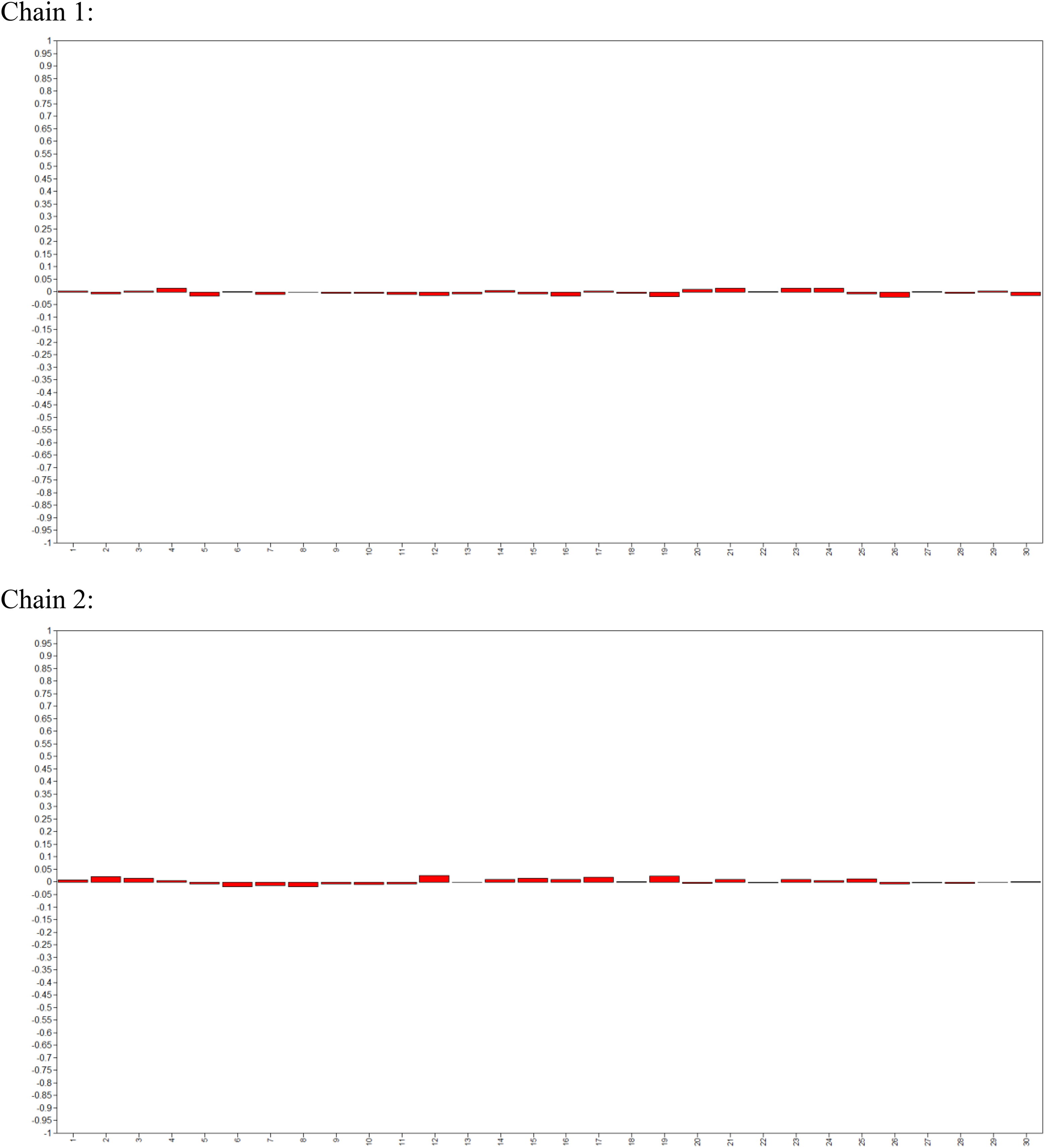
Bayesian autocorrelation plots.
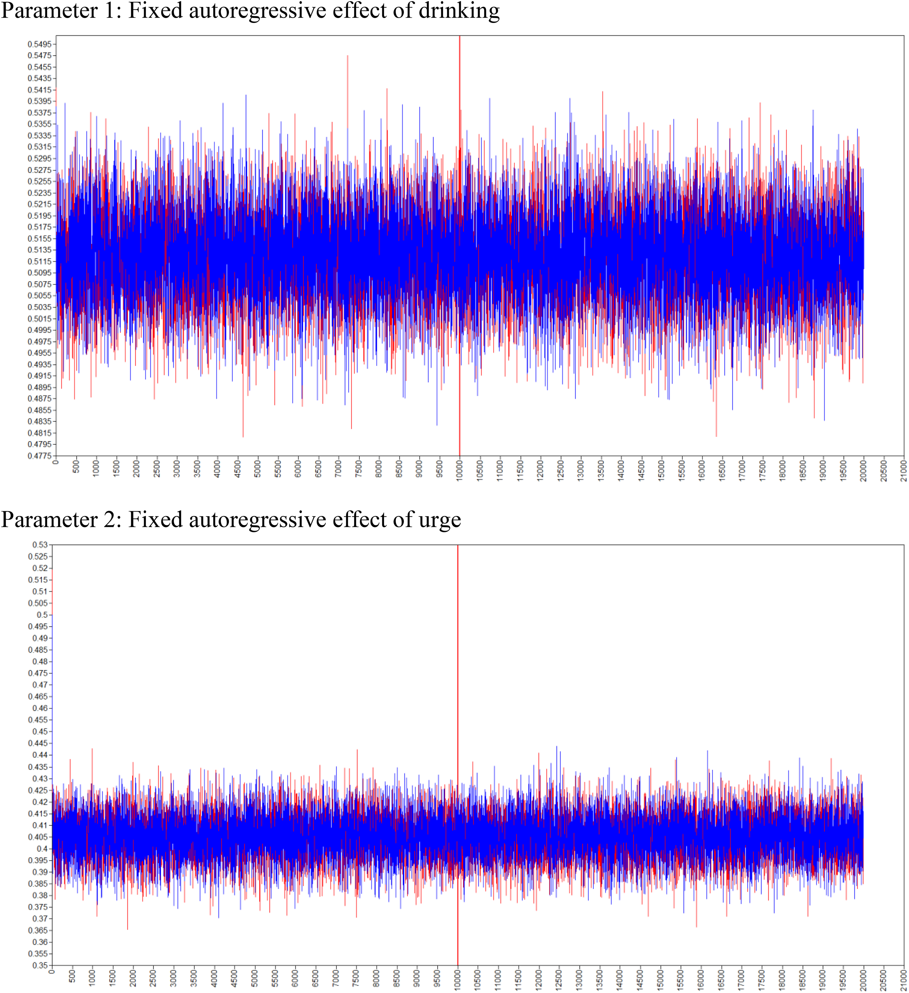
Trace plots.
Dynamic Structural Equation Modeling: Demonstrations
We provide three examples to demonstrate how to use DSEM to specify and estimate multilevel models for ILD in software Mplus 8.2. Syntax of all three examples are included in Appendix B (available in the online version of the journal). In data sets to be input to Mplus, lagged measurements (i.e., columns “Yt–1, i”, “Yt–2, i”, “Xt–1, i”, and “Xt–2, i” in Table 1) do not need to be manually created if DSEM will be used. Instead, users can use the “LAGGED” command in Mplus to identify time-lagged variables. In all three examples, we used the default, noninformative priors for model parameters since we had limited existing knowledge about these parameters (see Hamaker et al., 2018; B. Muthén, 2010, for the default priors used in Mplus for DSEM). We used 20,000 iterations in each example and a thinning of every 10th iteration. We used the default number of chains (i.e., two) and the default number of discarded iterations (i.e., the first half of each chain; also called burn-in period) in Mplus.
Example 1: Bivariate Time Series With Subject-Level Predictor and Outcome
In this example, we estimated a model with time series for two outcomes, a subject-level predictor, and a subject-level outcome. This example assumes that a researcher is interested in testing the reciprocal relationships between drinking and urge and how these reciprocal relationships are affected by neuroticism and in turn influence job performance (see Figure 3). The researcher also wants to account for other dynamic processes that may be involved. Therefore, the researcher specifies a model (see Equations B1–B12 in Appendix B available in the online version of the journal) that includes (a) random means of drinking and urge; (b) autoregressive relationships of drinking and urge, respectively; (c) cross-lagged relationships between drinking and urge; (d) random within-participant residual variances of drinking and urge, respectively, and their covariance; (e) subject-level effects of neuroticism on means, autoregressive relationships, cross-lagged relationships, random within-subject variances, and covariance; and (f) subject-level effects of means, autoregressive relationships, cross-lagged relationships, random within-subject variances, and covariance on job performance. If a cross-lagged model or a latent growth model were used, it would be extremely cumbersome to specify these effects, particularly those described in (b) autoregressive relationships of drinking and urge, respectively, and (c) cross-lagged relationships between drinking and urge. Moreover, without using Bayesian methods, estimating the model parameters would take a long time and could yield biased estimates if observed mean centering is used for time-lagged predictors (Asparouhov et al., 2018). We used simulated Dataset 1 (see syntax in Appendix A, available in the online version of the journal) for this demonstration. Population true values of parameters are reported in Table 2, for comparing estimation results.
Results From Example 1.

Note: N = 21,000 at within-person level, and N = 200 at person level. The default for point estimate of central tendency of posterior distribution in Mplus is median. One can also request mean or mode using “POINT” command within “ANALYSIS.”
Researchers should first examine whether the model converged properly. “TECH8” command in Mplus is used to request printing the optimization history (including PSR values) and “PLOT” command to request Bayesian autocorrelation plots and trace plots for all model parameters (see Example 1 syntax in Appendix B, available in the online version of the journal). PSR values are mostly close to one for each parameter, suggesting that the number of iterations is sufficient. Bayesian autocorrelation plots for one of the parameters (i.e., fixed autoregressive effect of drinking) are illustrated in Figure 4. As shown in Figure 4, small autocorrelations are achieved in each chain even at a short interval for this parameter. Similar patterns are shown in autocorrelation plots for other parameters in the model. Therefore, we do not add extra thinning. Trace plots for two parameters (i.e., fixed autoregressive effects of drinking and urge) are illustrated in Figure 5. Inspecting the trace plots for each parameter suggests that there is no abnormality in model convergence process. Taking all three pieces of information together, we consider that model converged properly in this example.
As reported in Table 2, posterior distributions show that given the observed data, there is ample evidence for a positive cross-lagged relationship between urget–1 and drinkingt (in the posterior distribution, the peak is at .605, and the 95% credibility interval ranges between 0.585 and 0.625; i.e., π20 = .605, 95% CV = [0.585, 0.625]) and a positive cross-lagged relationship between drinkingt–1 and urget (π40 = .020, 95% CV = [0.003, 0.037]). These results suggest that urge and drinking positively reinforce each other over time. For those who are more neurotic, there is a stronger cross-lagged relationship between urget–1 and drinkingt (π21 = .289, 95% CV = [0.264, 0.315]), whereas there is close to null relationship between neuroticism and the cross-lagged relationship between drinkingt–1 and urget (π41 = .010, 95% CV = [–0.013, 0.034]). There is no evidence that the strength of the cross-lagged relationship between urget–1 and drinkingt is related to job performance (π75 = .315, 95% CV = [–0.425, 1.082]) or that the strength of the cross-lagged relationship between drinkingt and urget–1 is related to job performance (π77 = .528, 95% CV = [–0.030, 1.088]). Comparing the values in the true model to these estimates (see Table 2) suggests that DSEM captured the true population values well.
In addition to these effects of interest to the researcher, results also show that on average across all individuals, there are positive autoregressive relationships for drinking (π10 = .513, 95% CV = [0.497, 0.528]) and urge (π30 = .405, 95% CV = [0.386, 0.424]), and these autoregressive relationships vary across individuals for both drinking (variance of u1i = .007, 95% CV = [0.005, 0.010]) and urge (variance of u3i = .011, 95% CV = [0.007, 0.015]). These results together suggest that drinking and urge have day-to-day carryover effects that signal lack of self-regulation and these carryover effects vary from person to person. Furthermore, results show that neuroticism is positively related to the average amount of drinking (π Y 01 = .328, 95% CV = [0.195, 0.463]), the autoregressive relationship of drinking (π11 = .103, 95% CV = [0.082, 0.124]), and magnitude of within-person variability in drinking (π Y 51 = .209, 95% CV = [0.001, 0.422]), which in turn are related to job performance (π72 = .554, 95% CV = [0.481, 0.631] for average amount of drinking; π74 = .759, 95% CV = [0.042, 1.502] for autoregressive relationship of drinking; and π78 = .504, 95% CV = [0.457, 0.552] for within-subject variability of drinking). Finally, as reported in the bottom part of Table 2, the within-subject variability of drinking (variance of uY5i = 1.192, 95% CV = [0.978, 1.475]) and urge (variance of uX5i = 1.075, 95% CV = [0.867, 1.353]) and the association between fluctuation of drinking and fluctuation of urge (variance of u6i = 1.591, 95% CV = [1.258, 2.021]) vary across individuals.
Example 2: Univariate Time Series With Time-Varying Predictor, Trend, and Time-Varying Effects
In this example, we demonstrate how trend of the outcome variable and effect of time-varying predictors can be modeled simultaneously in a cross-classified model. This example assumes that a researcher is interested in the impact of urge (which could be triggered by negative workplace events) on drinking among newcomers after the carryover effect of drinking itself is accounted for. The researcher also expects that the effect of urge on drinking becomes weaker over time as newcomers develop coping skills. In addition, the researcher expects that drinking linearly decreases over time as newcomers adjust to the new environment. To test these hypothesized relationships, the researcher specifies a model (see Equations B13-B18 in Appendix B, available in the online version of the journal) that includes (a) an autoregressive relationship of drinking, (b) effect of time’s linear term on drinking, (c) effect of urge on drinking, (d) effect of time’s linear term on urge-drinking relationship at the time level, and (e) residual variances of drinking, trend, and urge-drinking slope at the person level. We used simulated Dataset 2 (see syntax in Appendix A, available in the online version of the journal) for this demonstration.
The model converged properly. As reported in Table 3, at the between-person level, there is evidence that urge is related to drinking (π10 = .437, 95% CV = [0.366, 0.509]), and this urge-drinking relationship varies across individuals (variance of u1i = .194, 95% CV = [0.158, 0.241]). There is evidence that the urge-drinking relationship becomes weaker as time goes by (ψ11 = –.100, 95% CV = [–0.100, –0.099]), and this relationship fluctuates over time (variance of w1t = .002, 95% CV = [0.000, 0.005]). Over time, there is a negative trend of drinking across all individuals (π20 = –.203, 95% CV = [–0.208, –0.198]), and this trend does not vary among individuals (variance of u2i = .000, 95% CV = [0.000, 0.000]). Note that when the data were generated, trend parameter was not given any variability across individuals in the true model (see Appendix A, available in the online version of the journal). Thus, it is not surprising that estimate for this parameter was zero. In reality, researchers can use region of practical equivalence (ROPE) to assess practical significance of an effect (Jebb & Woo, 2015).
Results From Example 2.

Note. N = 21,000 at within-person level, and N = 200 at person level.
Example 3: Univariate Time Series With Cycles
In the final example, we demonstrate how cycles can be accounted for in DSEM by coding cycles into predictor variables. This example assumes that a researcher wants to conduct supplemental analyses to test whether there are weekly cycles in drinking. The researcher specifies a simple model (see Equations B19 and B20 in Appendix B, available in the online version of the journal) that includes an autoregressive effect and predictors representing cycles coded using sine and cosine functions (see Example 3 syntax in Appendix B, available in the online version of the journal). We used simulated Dataset 3 (see syntax in Appendix A, available in the online version of the journal) for this demonstration. The model converged properly. Results show that weekly cycles do exist in drinking (coefficient for sine function: c2 = 1.311, 95% CV = [1.269, 1.353]; coefficient for cosine function: c3 = 2.140, 95% CV = [2.107, 2.173]). Based on these results, the researcher may want to add cycles as control variables in further supplemental analyses.
Discussion
Theoretical Development and Research Design Issues
As Collins (2006) pointed out, an ideal longitudinal research should include at least three well-integrated elements: (a) a well-articulated theoretical model of change observed using (b) a temporal design that affords a clear and detailed view of the process, with the resulting data analyzed by means of (c) a statistical model that is an operationalization of the theoretical model. (p. 507)
First, ILD are well suited to test theories that concern dynamic processes (Wang et al., 2016). Although organizational research is starting to pay more attention to process-oriented mechanisms, “time” is still missing from many theories in our research (Cronin & Vancouver, 2019; Kozlowski et al., 2013; Mitchell & James, 2001). To guide proper statistical analyses using ILD, theories should inform the specification of the statistical models, including the models described here. For example, by articulating the mechanisms underlying observed trajectories (e.g., self-regulation processes, emergence processes), theories would need to inform whether there is a trend in the ILD and in what functional form (e.g., linear or quadratic), whether and how the state of the variable at an earlier time relates to its state at a later time (i.e., autoregressive relationship), whether the variable goes through cycles or seasons and at what frequency, as well as how multiple variables influence each other over time with their own changes considered. Moreover, theories would need to explain whether these temporal relationships vary across subjects and if so, the antecedents and consequences at the subject level that are related to these between-subject differences.
Second, although ILD afford a closer look at a phenomenon of interest, without a strong research design, it is extremely difficult to draw causal inferences from data alone. Using the drinking study as an example, a researcher may measure drinking and urge regarding the same time period (e.g., this morning) at the same time at each measurement. In statistical analyses, the researcher treats urge as a time-varying predictor that concurrently influences drinking (i.e., urget to drinkingt) and finds evidence for a non-zero relationship. In this case, it is not convincing to claim that there is a causal effect of urge on drinking for at least two reasons: urge does not proceed drinking in the cross-sectional design at each measurement and urge and drinking could be influenced by the same third time-varying variable not even measured in the study. To establish a causal relationship, the researcher would need to measure variables in a way that allows the study to establish temporal precedence of the cause, have sufficient statistical power to detect the effects, and be able to rule out alternative explanations.
Finally, ILD often have a larger volume of information than panel design data and thus allow more explorative analyses, which is a great opportunity for organizational researchers. However, when the explorative analyses results are not examined again in future studies, it is impossible to know whether the patterns discovered in the explorative analyses only exist in one particular set of ILD or they represent relationships among the larger population. In addition, some explorative analyses may not be reported fully in the manuscripts. For example, since DSEM allows researchers to specify priors, it is possible to try multiple priors and report only the priors that generate posterior distributions consistent with the hypotheses (see further discussion in Zyphur & Oswald, 2015). These issues related to reproducibility and replicability are certainly not unique for research utilizing ILD. In research using less intensive data, there has been an ongoing discussion of how to properly conduct and report planned and explorative analyses (e.g., see Hollenbeck & Wright, 2017, for a discussion on harking, sharking, and tharking; see Simmons, Nelson, & Simonsohn, 2011, for discussion on p-hacking). One way to address the reporting problem is to encourage conducting and reporting robustness checks. For example, when a large sample is available, researchers can split the sample into two and use one as a holdout sample for cross-checking model specification and estimation procedures that should be robust across subsamples (e.g., a particular estimator used). However, the holdout sample would share similar properties as the main study sample and may not be able to help assess generalizability across contexts. More importantly, in our opinion, the increased space for explorative tests in ILD calls for more replication studies in general (see different types of replication studies described in Bettis, Helfat, & Shaver, 2016). In the drinking research example, the researcher may first inspect the data set and notice weekly cycles in drinking. The researcher then comes up with a theory to “predict” this weekly cycle, incorporates cycles in the statistical model, and demonstrates that the model with cycles fits the data better than the one without and parameters representing cycles have larger than zero coefficients. In addition to the ethical debates regarding whether the researcher should reveal the post hoc inclusion of cycles in the statistical model, another important issue here is whether the cycles reported in this one study are specific to the sample. To find answers to this question, we would need more replication studies. In summary, we recommend a programmatic way to studying dynamic processes with ILD.
Other Considerations and Caveats
Centering decisions
Centering is an important issue in multilevel models in general because researchers want to decompose within- and between-subject effects of time-varying covariates (Curran & Bauer, 2011). Like in any other multilevel models, choice of centering options can affect modeling results. In multilevel models for ILD, there are two centering issues (Asparouhov & Muthén, 2019; Curren & Bauer, 2011): centering a concurrent covariate (i.e., Xti) and centering the time-lagged outcomes (i.e., Yt–1, i, Yt–2, i, etc.). There are four centering options for these two types of within-subject level predictors: (a) no centering, (b) grand mean centering, (c) centering by the observed sample mean of each subject (e.g.,
Prior simulation work demonstrates that latent mean centering using Bayesian estimation generally outperforms other centering options (see details and exceptional situations in Asparouhov et al., 2018; Asparouhov & Muthén, 2019). This is also the case for multilevel models for ILD. For example, estimates of the average autoregressive effects are more accurate when using latent mean centering with Bayesian estimator, which eliminates Nickell’s bias. In addition, missing data in time-varying covariate can be accounted for in DSEM through specifying multivariate time series models. In summary, the approach used in DSEM (i.e., latent mean centering with Bayesian estimator) effectively addresses potential issues associated with centering.
Measurement model
One advantage of DSEM is that it allows specifying measurement model in addition to the structural relationships (Asparouhov et al., 2018). Indictors of latent outcome variables that change over time can be categorical or continuous variables. In the drinking study, a researcher may want to include multiple continuous indicators of urge that are measured by having participants rate on a 5-point Likert scale how accurately a few statements describe their cognitive and emotional states at work. Categorical indicators can be included, such as, employment status (employed vs. unemployed) and promotion decision (promoted vs. not promoted). In addition to categorical indicators, latent categorical variables can be included as predictors or outcomes as well (e.g., whether drinking trajectories captured by ILD predict movers vs. stayers later in subjects’ careers). Developed under the general latent variable analyses framework, DSEM is apt at incorporating these additional components.
Missing data and unbalanced time structure
When all subjects go through the same design regarding time (i.e., same starting point, same time interval between measurements, same ending point), some subjects may miss some of the measurements. Similar to data from panel studies, missing data in ILD are better handled by modern missing data analyses techniques (e.g., full information maximum likelihood estimation) than listwise deletion (i.e., removing subjects with any missing values in any repeated measurements), removing any pair of measurements with missing in lagged proceeding measurements (e.g., removing any pair of Yt–1 and Yt when Yt–1 is missing), or using observed subject mean imputation (i.e., using a subject’s sample mean to fill in any missing measurements). To model missing data in DSEM, a researcher needs to clearly code the time of measurement for each subject. In Bayesian model estimation process, a missing value at a particular measurement point is sampled from a conditional posterior distribution of this measurement that depends on other data in the series and other parameters in the model (Hamaker et al., 2018). This procedure assumes that missing data occurs through missing at random (e.g., missing data in drinking are correlated with other variables in the study and are not correlated with values of drinking per se).
In addition to modeling missing data from studies with identical designs for all subjects, this procedure can also be used to account for unequal measurement time intervals across subjects. For example, due to logistics constraints, a researcher may be able to measure drinking only once every other day among a subgroup of participants. 8 In the data analyses phase, the researcher can “force” measurement intervals to be equal for all subjects by using the same interval to define the time of measurements for all subjects and code the measurements not available as missing data. Simulation studies suggest that quality of estimates from DSEM with missing data depends on various factors, including the amount of missing data, complexity of the model, and length of interval used to code uneven measurements (Asparouhov et al., 2018). Researchers generally should choose a time interval that is meaningful given the research context (e.g., use one day as the interval in the drinking study).
Sample size
Schultzberg and Muthén (2018) conducted a simulation study to evaluate the sample size requirements of univariate AR(1) model with random mean, autoregressive relationship, and random within-subject residual variance using DSEM. Results suggest that when a trade-off has to be made, a larger subject size (e.g., number of participants included in the drinking study) with a smaller number of measurements (e.g., number of days participants report drinking) should outperform a smaller subject size and a larger number of measurements (in terms of accuracy and reliability of parameter estimates and estimation efficiency). In addition, when random relationships between within subject–level variables (e.g., cross-lagged relationships between drinking and urge) are used as Level 2 predictors, a larger subject size is required than when these random relationships are used as outcomes. When multiple complex modeling components are included simultaneously (e.g., relationships among random autoregressive relationships, random within-subject residual variances and Level 2 outcomes), Schultzberg and Muthén recommend having at least 200 subjects and at least 100 measurements for each subject. More studies are still needed to fully understand sample size requirements for more complicated multilevel models for ILD.
Limitations of DSEM
As a method still in its infancy, DSEM is not without limitations. For example, when autoregressive relationships for categorical variables are included in DSEM, such autoregressive relationships have to be specified using additional latent factors rather than having direct relationships between observed variables (Asparouhov et al., 2018). In addition, depending on the theory and phenomenon of interest, other analytic approaches for ILD may be more efficient than DSEM. First, DSEM is a type of discrete time model; estimates of the parameters are tied to the time interval specified in the model (Dormann & Griffin, 2015; Hamaker et al., 2018). Thus, when the processes studied evolve continuously over time and extremely high-frequency measurements are available (i.e., measurements almost approaching “continuous” assessment), continuous time models (e.g., differential equation models; Hu, Boker, Neale, & Klump, 2014; Steele & Ferrer, 2011) are more appropriate than DSEM. Second, although cycles (or frequencies) can be accounted for in DSEM, DSEM mostly addresses questions about time domain. Time series data can be examined by time domain models (where the processes over time are of interest) or frequency domain models (where the processes at different frequencies are of interest). Although time domain models and frequency domain models can be used to describe the same time series, frequency domain techniques (e.g., spectral analysis; Shumway & Stoffer, 2017) may be more efficient when multiple underlying cyclical components (e.g., cycles in sleep waves or social interactions; Sadler, Gunn, Ethier, Duong, & Woody, 2009) are of interest.
Conclusion
While development in theories has called for more longitudinal studies for theory testing and advances in research methods have provided us access to higher frequency data, there has been limited discussion on analytic tools for intensive longitudinal data in organizational research. We introduce dynamic structural equation modeling to organizational researchers, which integrates multilevel modeling, time series modeling, structural equation modeling, and time-varying effects modeling and uses Bayesian methods. Based on the illustration of this new analytic method, we hope future research can employ this tool to test temporal-oriented theories and inform organizational practices concerning dynamic processes.
Supplemental Material
Supplemental Material, Revised_online_supplemental_material_(Appendix_A_B) - Intensive Longitudinal Data Analyses With Dynamic Structural Equation Modeling
Supplemental Material, Revised_online_supplemental_material_(Appendix_A_B) for Intensive Longitudinal Data Analyses With Dynamic Structural Equation Modeling by Le Zhou, Mo Wang and Zhen Zhang in Organizational Research Methods
Footnotes
Declaration of Conflicting Interests
The author(s) declared no potential conflicts of interest with respect to the research, authorship, and/or publication of this article.
Funding
The author(s) disclosed receipt of the following financial support for the research, authorship, and/or publication of this article: Le Zhou’s work on this research was supported by the Lawrence Fellowship from the Carlson School of Management, University of Minnesota and the National Science Foundation (Grant No. 1533151). Mo Wang’s work on this research was supported in part by the Lanzillotti-McKethan Eminent Scholar Endowment.
Supplemental Material
Supplemental material for this article is available online.
Notes
References
Supplementary Material
Please find the following supplemental material available below.
For Open Access articles published under a Creative Commons License, all supplemental material carries the same license as the article it is associated with.
For non-Open Access articles published, all supplemental material carries a non-exclusive license, and permission requests for re-use of supplemental material or any part of supplemental material shall be sent directly to the copyright owner as specified in the copyright notice associated with the article.
