From Data to Causes I: Building A General Cross-Lagged Panel Model (GCLM)

Occasion effects α t

To model causal effects in panel data, it is important to account for overall changes in a sample across occasions, which may be due to a variety of aggregate factors that are unrelated to lagged effects (i.e., AR and CL terms). We account for these with an occasion effect α t . For example, if y i t were work stressors, α t could capture aggregate change in work demands such as seasonal effects for all employees; if y i t were organization performance, aggregate change in industry-related factors could be captured by α t ; if y i t were national income, the global financial crisis could be captured by α t . Such effects are often controlled using T – 1 dummy variables that code for occasion of measurement, but as we show later, an SEM automatically accounts for α t with observed-variable intercepts.

Autoregressive (AR) effects β y 1 ( y ) and β x 1 ( x )

A key part of the cross-lagged model are AR effects that link the past and future (see Figure 1). With this approach, a unit’s current state is a function of its past, so x i t and y i t depend on x i t − 1 and y i t − 1 with AR terms β x 1 ( x ) and β y 1 ( y ) , respectively; we show a lagged path from a past y i t − h to a future y i t as β y h ( y ) . These effects show how a process unfolds, reflecting the fact that the current states of a system do not spontaneously arise. Instead, they depend on past states, such as current national income depending on past income, current organization performance depending on past performance, or current individual counterproductive behaviors depending on past behaviors.

An AR term β y 1 ( y ) captures this as a proportion of the past that persists directly to the next occasion ( y i t − 1 is multiplied by β y 1 ( y ) ). Thus, if β y 1 ( y ) = 0 , it implies current levels of national income, organization performance, or individual behaviors are independent of past levels, but as β y 1 ( y ) → 1 , the present increasingly resembles the past. This can be seen in Figure 1 by tracing AR paths as indirect effects of the past, which can be though of as a kind of persistence, momentum, inertia, memory, or carryover. Alternatively, inverse meanings (e.g., 1 − β y 1 ( y ) ) can be adopted, such as forgetting, decay, entropy, regulatory strength, or regression to the mean, because as β y 1 ( y ) → 0 , past states fade more quickly. On the other hand, negative AR terms can indicate a pendulum-like process, wherein values on a variable tend to alternate between positive and negative over time—a type of “anti-dependence”—such as in a system that responds by counteracting past states (e.g., cycles of activity vs. respite).

We return to AR terms when treating long-run effects, and Online Appendix B treats the special case of AR ≥ 1, but for now, we lay a foundation for seeing CL effects as causal by noting that AR terms help control for some confounds. For example, employees may engage in counterproductive work behaviors as a matter of habit rather than due to increases in work stressors, so controlling for past counterproductive work behaviors with AR terms is relevant. Similarly, organizations may experience high performance due to persistent market forces rather than changes to HR practices, so again, performance AR terms may be useful. Also, nations may experience low well-being that persists for reasons that may be unrelated to decreases in national income. Thus, AR terms reflect persistence, but they also control for a variable’s past levels to help avoid drawing erroneous causal conclusions using CL terms.

This understanding of AR terms motivates a discussion of CL effects, but before this, it is important to note that some processes cannot be modeled by a single AR term, such as lagged effects that take longer than a lag h = 1 to appear or complex processes that can be modeled by both a positive and negative AR term at different lags. As Figure 1 shows, AR terms recursively link the past to the future (e.g., y i t − 2 impacts y i t indirectly via y i t − 1 ), but some processes may require not only an indirect effect from y i t − 2 to y i t via y i t − 1 but also a direct effect β y 2 ( y ) of y i t − 2 on y i t . The latter is a higher-order lag, which would be a model with an AR “lag order” of 2, noted as p in an AR(p) model—an AR(2) model here. In this case, researchers may combine all p AR terms that impact a future y (e.g., β y . ( y ) = β y 1 ( y ) + β y 2 ( y ) ), which is equivalent to combining all p AR terms that emanate from a past y and allows a single AR term to be used as a kind of shorthand to infer about the AR dynamics affecting a future observation of y (e.g., on the whole persistent with a positive β y . ( y ) or anti-persistent with a negative value). We discuss issues related to higher-order lags later, and our online Excel file can automate Mplus input for models with varying lag orders.

Cross-lagged effects β y 1 ( x ) and β x 1 ( y )

By including AR terms, it becomes posible to use the past of one variable to uniquely predict the future of another. Such CL effects imply that each unit’s current state is a function of its past on other variables; so for example, x i t is predicted by y i t − 1 with a CL effect β y 1 ( x ) , and y i t is predicted by x i t − 1 with β x 1 ( y ) ; a path from x i t − h to y i t is β x h ( y ) . These effects enact a temporal order that is consistent with causation, which is partly used to justify treating CL terms as causal. Often called Granger causality, the idea is that if a predictor uniquely accounts for the future along a variable, then this can serve as provisional evidence of causation (Granger, 1969, 1980, 1986, 1988).

With this logic, CL terms are used to infer causality, but as Figure 1 shows, they only imply a “short-run” effect as a direct effect of the past on the future. Just like AR terms, these depict a system’s short-run behavior, with implications for CL terms ≥ 1, as noted in Online Appendix B. Yet, investigating long-run behavior requires examining how the past indirectly affects the future along all AR and CL paths simultaneosuly (e.g., the total effect of an initial x i 1 on y i 2 , y i 3 , etc.). As we show later, such long-run effects map onto key hypotheses such as “a vicious cycle” among work stressors and behavior (Meier & Spector, 2013, p. 537), or if “human capital investments…yield a high return” (Van Iddekinge et al., 2009, p. 840), or if “people [do] not adapt to income increases” (Diener et al., 2013, p. 275).

We will cover long-run hypothesis tests when we treat impulse responses. For now, we note that just like AR effects, higher-order CL terms may be needed for some processes. For example, work stressors may have delayed or complex effects on counterproductive work behaviors, requiring a second lag c = 2 in a CL(2) model, such as an effect β x 1 ( y ) of x i t − 1 on y i t and a direct effect β x 2 ( y ) of x i t − 2 . Here, a single CL term can be used as a shorthand for all CL effects associated with a future y or similarly, all CL effects emanating from a past x ( β x . ( y ) = β x 1 ( y ) + β x 2 ( y ) ). We later show how to specify and select models with higher-order CL lags and how to test effects among variables in more nuanced ways using impulse responses.

Impulses u i t

The model also includes a residual term to allow units to differ over time due to random inputs (Denrell, Fang, & Liu, 2014). Although residuals are often taken for granted in regression, in cross-lagged models, they actually have an important substantive role that requires some theoretical prefacing. For example, consider that rules and routines guide social entities but behavior and events are never predictable as novelties emerge over time (Becker, Knudsen, & March, 2006; Weick, 1998). The same is true for larger economic changes (Lütkepohl, 2015), which are typically unpredictable or even a priori unexplainable (Cochrane, 1994). This is echoed by research efforts in social science that fail to explain substantial variation because of the stochastic nature of many phenomena (Abelson, 1985).

To capture such random inputs for each unit i at a given occasion t, we include a random term u i t , so x i t and y i t are functions of u i t ( x ) and u i t ( y ) with variances ψ u t ( x ) and ψ u t ( y ) , respectively. Put simply, u i t represents random events that make observations unique, such as events that raise/lower a person’s work stressors by 1 point, or organization performance, or national income at a time t (i.e., u i t = ± 1 ). Thus, although u i t is often called a residual or a disturbance and ψ u t is a residual variance, we call u i t an impulse and ψ u t an impulse variance because they do not imply error. Instead, they capture a unit-specific “shock” or an unpredictable “surprise” in the system being modeled over time (Stock & Watson, 2001). This conceptualization will later be used to facilitate an understanding of causality in our model.

Before this, however, we note that an impulse u i t may be nonindependent if a shock affects multiple variables. Such common causes can still be random, such as unpredictable changes in work assignments causing simultaneous change in work stressors and behavior, or unpredictable changes in organization leadership causing change in both HR practices and performance, or unpredictable events in a nation causing change to SWB and income. We call such effects a co-movement, which can be modeled in various ways (Bai & Ng, 2008; Bernanke, Boivin, & Eliasz, 2005; Stock & Watson, 2005, 2011). As Figure 1 shows, we use a covariance ψ u t ( x y ) among impulses u i t ( x ) and u i t ( y ) , but again, ψ u t ( x y ) is not a residual covariance and instead represents something unique in a unit i at a time t that is shared by two variables.

The co-movement ψ u t ( x y ) aids in interpreting CL effects as causal by accounting for predictor covariance—this is how regression accounts for confounds. To understand this, we make the crucial point that AR and CL terms can be seen as modeling the persistence of past impulses (Hamaker, 2005), essentially reflecting how long these last as they propagate into the future. For example, how long does a random change to work stressors, organization performance, or national income last—conversely, how long until it fades? Figure 1 shows this by path tracing from an impulse to future observations on AR and CL paths. Impulses persist longer if AR and CL terms are larger (persisting indefinitely if an AR term β y 1 ( y ) = 1 ); conversely, regression to the mean occurs more quickly if they are smaller. We treat this further in Online Appendix B but for now emphasize that a co-movement ψ u t ( x y ) can help in understanding AR and CL terms as capturing the independent effects of past impulses.

Summary and limitations

The cross-lagged model has many useful properties. It controls for occasion effects α t while modeling system dynamics with AR effects β y 1 ( y ) and β x 1 ( x ) and CL effects β y 1 ( x ) and β x 1 ( y ) . Here, AR terms are meant to indicate the proportion of the past that directly persists to the future on a variable, which is meant to serve as a control when assessing direct effects of other variables with CL terms. What remains should be random impulses u i t ( x ) and u i t ( y ) with variances ψ u t ( x ) and ψ u t ( y ) and a co-movement ψ u t ( x y ) , all of which are meant to reflect factors uniquely affecting a unit i at a time t—again, we assume that x and y are error free, but we later note that this can be easily addressed in SEM.

However, there are two limitations of this approach that motivate a GCLM. First, all units are treated as if they were the same in the long run—Figure 1 does not reflect any stable between-unit differences. This is anathema to organization research in which individual and organizational differences such as personality or culture are well recognized and units differ systematically over time. By failing to model stable factors, they will be confounded with the system dynamics that should be reflected by AR and CL terms (Hamaker et al., 2015). Thus, a more general model is needed to account for stable factors, which we will call unit effects.

The second limitation is that the dynamic process linking the past and the future via AR and CL terms is assumed to follow a simple, indirect-effects structure. As we noted, AR and CL terms depict persistence (or regression to the mean) of a past impulse, but this might persist (or fade) in complex ways. Thus, a more general model may help to overcome the indirect-effects structures associated with AR and CL terms, which we will treat in the next section using moving average (MA) and cross-lagged moving average (CLMA) terms.

Unit Effects λ t η i

Researchers often seek to explain two distinct causes of variation in people, organizations, and larger entities. On the one hand there is variation within units as each one changes relative to itself over time; AR, CL, and impulse terms capture these dynamics as units experience random shocks that persist via AR and CL paths. On the other hand, units may systematically differ from each other, producing variation between units of analysis due to factors that create stability rather than occasion-specific change.

To elaborate, if a unit i is a person, psychological factors can explain stability over time, including stable patterns of embodied cognition (Barsalou, 2008), social roles and norms (Andersen & Chen, 2002; Fournier, Moskowitz, & Zuroff, 2008), cognitive ability (Deary, Pattie, & Starr, 2013), personality or affective traits (Matthews, Deary, & Whiteman, 2003), and habits of thought/action that emerge in stabilized person-environment interactions (Fleeson, 2001; Mischel, & Shoda, 2008; Neal, Wood, & Quinn, 2006). Alternatively, if i is a group, organization, or a nation, substantial scholarship treats how collectives emerge as stable entities, such as by the formation of institutions (March & Olsen, 1989) and collective routines to guide social and material processes (Feldman & Orlikowski, 2011; Winter, 2013).

Such causes of between-unit differences are not the same as causal effects among variables as they change over time (Allison, 2005; Hamaker et al., 2015). Instead, between-unit differences are akin to unit-specific trends (e.g., long-run averages) that systematically differentiate units over time (i.e., between-unit differences). These should not confound the AR, CL, and impulse terms that represent perturbations around any such trends (see Online Appendix B) because stable factors are constant by definition and thus do not have a clear role in models of causality over time. To account for this, we treat each unit i as a function of unit-specific factors that are constant or nearly constant over T, modeled as a unit effect η i , so x i t and y i t are functions of η i ( x ) and η i ( y ) with variances ψ η ( x ) and ψ η ( y ) , respectively.

Unlike u i t , η i captures factors that make a unit similar to itself (rather than different) over time. This makes η i similar to a familiar common factor, which some researchers may think of as a “random intercept” in a multilevel model (see Hamaker et al., 2015). However, by including a covariance ψ η ( x y ) for unit effects (see Figure 2), stable factors are controlled when estimating AR, CL, and impulse terms; in econometrics, this is often called a “fixed effects” model because covariance among lagged predictors and unit effects is accounted for. Indeed, this covariance is crucial for holding stable factors constant across occasions.

OPEN IN VIEWER

Figure 2.

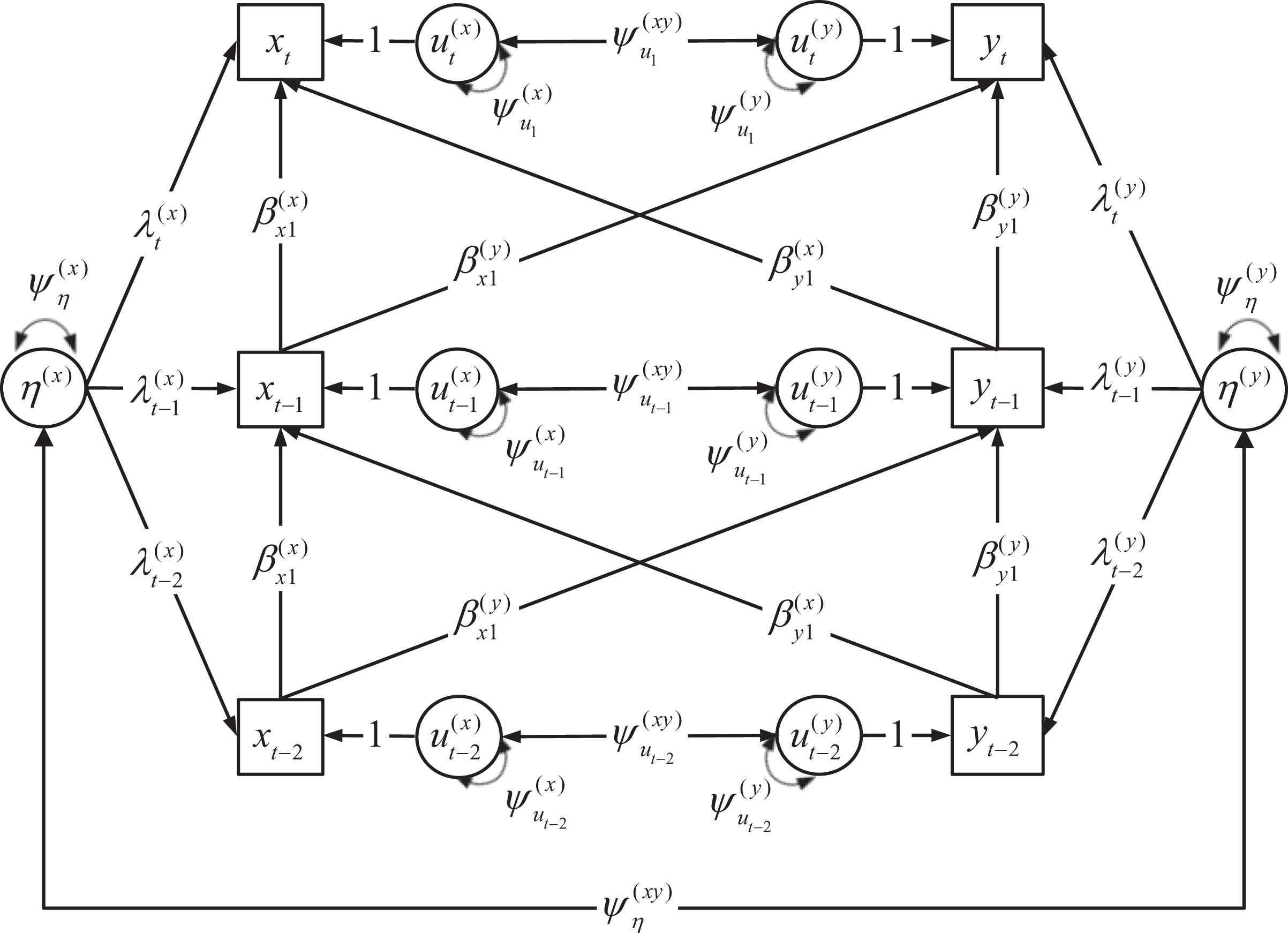
An AR(1)CL(1) model with unit effects.

Although everything changes with time, we model η i because ignoring it assumes that no stable between-unit differences exist (Bond, 2002; Shrout, 2011), which may be difficult to justify (Roberts & DelVecchio, 2000). This said, there are reasons to allow the effect of η i to vary over time. For example, situations differ in their effects on individual behavior, with constraining situations altering trait expressions (Cooper & Withey, 2009; Fleeson, 2004; see also Kanfer & Ackerman, 1989). Larger systems also change in how enduring characteristics are expressed (Gersick & Hackman, 1990; Kirkman & Rosen, 1999). We model such time-varying effects with occasion-specific “factors loadings” λ t ( x ) and λ t ( y ) :

x i t = α t ( x ) + λ t ( x ) η i ( x ) + β x 1 ( x ) x i t − 1 + β y 1 ( x ) y i t − 1 + u i t ( x )

3

y i t = α t ( y ) + λ t ( x ) η i ( y ) + β y 1 ( y ) y i t − 1 + β x 1 ( y ) x i t − 1 + u i t ( y )

4

This can be seen as a λ t × η i interaction, with either “an aggregate shock [ λ t ] that has individual-specific effects [ η i ], or a permanent characteristic [ η i ] that has changing effects over time [ λ t ]” (Arellano, 2003, p. 63; Bai, 2009, 2013; Moral-Benito, 2013). The common scenario where λ t = 1 has been called mean stationarity (Bun & Sarafidis, 2015), with various ways to proceed if it does not hold (see Ahn, Lee, & Schmidt, 2001, 2013; Nauges & Thomas, 2003). We avoid this assumption, but as we note later, it can be imposed by fixing λ t = 1 (except at a first occasion λ t = 1 , which as we note later is freely estimated to reflect that η i is actually a unit-specific average adjusted by AR/CL terms; Hamaker, 2005).

Moving average effects δ x 1 ( x ) and δ y 1 ( y )

To generalize model dynamics, we now introduce MA and CLMA terms. The idea motivating these is that long-run and short-run dynamics may be different as impulses persist/fade over time, but AR and CL terms imply equivalent long- and short-run dynamics as a single set of parameters linking the past to the future. Because AR and CL terms imply impulse persistence, relying on only them to capture system dynamics is akin to assuming that unexpected changes persist or fade multiplicatively vis-à-vis AR and CL terms. This can be modified by making the future a direct function of past impulses, which is how MA and CLMA terms modify the typical cross-lagged model.

We begin with MA terms, which modify AR paths by making observations a direct function of past impulses (Box et al., 2008; Hamaker, Dolan, & Molenaar, 2002). This allows MA terms to modify the short-run persistence of an impulse, whereas AR (and CL) terms still reflect long-run dynamics. As Figure 3 shows, x i t is a function of u i t − 1 ( x ) with an MA term δ x 1 ( x ) and y i t a function of u i t − 1 ( y ) with an MA term δ y 1 ( y ) ; a path from u i t − h ( y ) to y i t is δ y h ( y ) :

x i t = α t ( x ) + λ t ( x ) η i ( x ) + β x 1 ( x ) x i t − 1 + β y 1 ( x ) y i t − 1 + δ x 1 ( x ) u i t − 1 ( x ) + u i t ( x )

5

y i t = α t ( y ) + λ t ( y ) η i ( y ) + β y 1 ( y ) y i t − 1 + β x 1 ( y ) x i t − 1 + δ y 1 ( y ) u i t − 1 ( y ) + u i t ( y )

6

OPEN IN VIEWER

Figure 3.

An AR(1)CL(1)MA(1) model with unit effects.

By including MA terms, generality is added to the way that dynamic processes can be modeled—specifically, by allowing MA terms to modify the way AR terms imply short-run persistence of impulses. This is seen by path tracing in Figure 3, where short-run persistence of an impulse is a sum of MA and AR terms (i.e., a total effect of u i t − 1 ( y ) on y i t is β y 1 ( y ) + δ y 1 ( y ) ), but AR (and CL) terms determine long-run dynamics as an impulse persists beyond the MA term into the future. The key to understanding how this works is by recognizing that an impulse can only travel along an MA term once, whereas AR and CL terms repeatedly link the past to the future over time. To show the value of differentiating short-run and long-run dynamics, we elaborate on two possible cases: (a) After an unexpected change in the form of an impulse, a system may stay perturbed in the short run but then rapidly adapt later versus (b) a system that adapts rapidly in the short run but then adapts very slowly later on.

To explain the first case, consider that as MA terms become more positive ( δ y 1 ( y ) > 0 ), it allows for short-run persistence of a past impulse while still allowing small AR terms to imply very weak long-run persistence. In the extreme case that AR terms equal 0, MA terms can reflect the persistence of an impulse to the next occasion t + 1 only, such as if changes in work stressors, HR practices, or national SWB persist to the next occasion but regress to the mean by the second occasion t + 2. This case could be common because individuals and organizations can fully adapt to the unexpected in some cases (Becker et al., 2006; Frederick & Loewenstein, 1999; Levitt & March, 1988), as can entire nations when agents respond in real-time to policy changes (see classic thought in Lucas, 1976).

In the second case, adaptation may occur rapidly at first but then slow over time. For example, there may be short-run adaptive responses to changes in counterproductive work behaviors (e.g., management interventions), organizational performance (e.g., increased competition), or national income (e.g., less stringent budget controls), but if these responses fade or become ineffective, then what remains of the initial change may persist. This is made possible by MA terms because as they become more negative (i.e., δ y 1 ( y ) < 0 ), the short-run persistence of an impulse is reduced while positive AR terms allow what remains to persist. Consider if an AR term β y 1 ( y ) = .95 were combined with an MA term δ y 1 ( y ) = − .75 , allowing the persistence of an impulse u i t − 2 ( y ) to be a small β y 1 ( y ) + δ y 1 ( y ) = .2 at the next occasion y i t − 1 . Yet, this would persist due to the AR term, with an effect of u i t − 2 ( y ) on y i t being ( β y 1 ( y ) + δ y 1 ( y ) ) β y 1 ( y ) = .2 × .95 = .19. Alternatively, if an AR term β y 1 ( y ) = 1 , the past would never fade in a system that is permanently impacted by its past (see Online Appendix B for insights).

To add additional generality to the model, higher-order MA lags may be included for q MA effects in an MA(q) model. Here, the sum of all MA terms is a shorthand for how MA effects from a single past u modify short-run persistence ( δ y . ( y ) = δ y 1 ( y ) + δ y 2 ( y ) ), with the total short-run persistence of an impulse then being β y . ( y ) + δ y . ( y ) . As noted in the following, choosing an AR(p) and MA(q) model can be done by model checking, but theory and past findings are also key (Allen & Fildes, 2001, 2005; Armstrong, 2001, 2005, 2007, 2012; Armstrong, Green, & Graefe, 2015). Often, simpler models are better (Green & Armstrong, 2015), and “we rarely seem to meet situations for which either p…or q need to be greater than 2. Frequently, values of zero or unity will be appropriate” (Box et al., 2008, p. 102).

Cross-lagged moving average effect δ y ( x ) and δ x ( y )

Just as AR and MA terms allow modeling a separate short-run and long-run dynamic structure, Figure 4 shows that the structure associated with CL terms can be extended analogously by making each unit’s standing on an observed variable a direct function of other variables’ past impulses. We call these CLMA terms, which arise when x i t is regressed on u i t − 1 ( y ) to estimate δ y 1 ( x ) and y i t is regressed on u i t − 1 ( x ) to estimate δ x 1 ( y ) ; a path from u i t − h ( x ) to y i t is δ x h ( y ) . With single-order lags for all terms, we refer to this full GCLM as an AR(1)MA(1)CL(1)CLMA(1) model:

x i t = α t ( x ) + λ t ( x ) η i ( x ) + β x 1 ( x ) x i t − 1 + δ x 1 ( x ) u i t − 1 ( x ) + β y 1 ( x ) y i t − 1 + δ y 1 ( x ) u i t − 1 ( y ) + u i t ( x )

7

y i t = α t ( y ) + λ t ( y ) η i ( y ) + β y 1 ( y ) y i t − 1 + δ y 1 ( y ) u i t − 1 ( y ) + β x 1 ( y ) x i t − 1 + δ x 1 ( y ) u i t − 1 ( x ) + u i t ( y )

8

OPEN IN VIEWER

Figure 4.

A full GCLM, AR(1)MA(1)CL(1)CLMA(1) model with unit effects.

By including CLMA terms, the model changes how causal effects can be understood. As noted previously, lagged effects can be seen as implying an effect of past impulses on future observed variables. In turn, just as the short-run persistence for a variable becomes AR+MA, the short-run effect of one variable on another becomes CL+CLMA. As Figure 4 shows, u i t − 1 ( x ) impacts y i t via CL and CLMA paths, so this is akin to estimating an effect of u i t − 1 ( x ) on y i t as the short-run effect β x 1 ( y ) + δ x 1 ( y ) . The idea here is that impulses can be treated as causes, which has been called Granger-Sims causality (Kuersteiner, 2010; Lechner, 2010).

This type of causality uses an interesting through experiment to ground it: Consider that if impulses are random, then it is as if a natural experiment were done at each occasion by randomly assigning units to a new level on a variable (e.g., u i t = + 1 ). Thus, impulses act as a conceptual randomization device, with CL+CLMA terms showing the short-run effects of random interventions (see Dufour, Pelletier, & Renault, 2006; Dufour & Renault, 1998; Dufour & Tessier, 1993; Lütkepohl, 1993; Sims, 1980). Indeed, longitudinal methods that use planned or natural experiments can rely on this logic by using treatment variables as predictors of random impulses (i.e., putting a time-varying treatment variable “behind” each random impulse; Angrist & Kuersteiner, 2011; Bojinov & Shephard, 2017; Stock & Watson, 2018). Of course, not everyone endorses the idea that impulses approximate randomization, but the fact that cross-lagged models are common and can be shown to rely on past impulses (see Online Appendix B) may help readers appreciate this kind of thought experiment.

The issue of causality aside, CLMA terms offer pragmatic value by allowing complex forms of dependence among variables. We treat this by analogizing the two previous MA cases. The first involved delayed adaptation, such that an unexpected change in a variable has an effect on the future of another, but adaptation then limits the duration of effects. This could be a case of short-lived effects of work stressors on counterproductive behaviors, HR practices on performance, or national income on SWB as each system adapts to the change. Here, an impulse u i t − 1 ( x ) may have a large positive CLMA term but a small CL term associated with y i t , so the early effect does not “repeat” at each future occasion of x. Indeed, as Figure 4 shows, if AR and CL terms were zero, MA and CLMA terms can model a system that fully adapts to previous impulses in all modeled variables (i.e., regression to the mean at t + 2).

The second case involved a small short-run effect that is highly persistent, such as a reverse-causal case of counterproductive behaviors affecting work stressors, organizational performance affecting HR practices, or national SWB affecting income, but with each effect being small yet long-lived over time. For this, an impulse u i t − 1 ( x ) may have a negative CLMA term δ x 1 ( y ) = − .75 and a large positive CL term β x 1 ( y ) = .95 associated with the outcome y i t . In this case, the short-run effect is positive and small β x 1 ( y ) + δ x 1 ( y ) = .20 , but this small effect can persist via CL (and AR) terms due to the large β x 1 ( y ) = .95 (see also Online Appendix B).

The point is that CLMA terms add generality to the kinds of dynamics that can be modeled. For this purpose, researchers may include l higher-order CLMA terms in a CLMA(l) model, such as if l = 2 for a CLMA(2) model. Again, the CLMA effects from a single past u can act as a kind of shorthand indicating how CLMA terms modify short-run effects ( δ x . ( y ) = δ x 1 ( y ) + δ x 2 ( y ) ), which in turn implies that an overall short-run effect of x’s impulses on y is β x . ( y ) + δ x . ( y ) . Given the potential complexity of models with such lags, we now offer ways to simplify hypothesis testing with the GCLM.

Substantive checking

We first examine the SWB dynamics, with an AR(1)MA(1) structure in all four models. As expected, the persistence of impulses quickly falls (top-left of Figures 5a-5d), with impulses almost entirely faded by the fourth future year. Also, 95% CIs include zero by the second year, so statistical significance exists only for the direct effect of a past impulse. In Table 3, this is the combined AR and MA term β y 1 ( y ) + δ y 1 ( y ) , which ranges from .535 to .595, so only 53.5% to 59.5% of a previous year’s impulse persists to the next year. Also, AR parameters β y 1 ( y ) range from .226 to .423, implying mean-reversion ( β y 1 ( y ) < 1 ). Finally, the time-varying unit effects λ t ( y ) are in a range consistent with stable unit effects, with the first λ t = 1 ( y ) being large, as expected, and those in future occasions ranging from .455 to .765. In sum, all results show an expected mean-reverting process, and meaningful unit effects imply stability over time. Therefore, substantively, all models seem appropriate.

On the other hand, income dynamics tell a different story (see top-right of Figures 5a-5d). The AR(1)MA(1) and AR(2)MA(2) models in Figures 5a and 5d imply mean-reversion, with Table 3 showing the AR(1)MA(1) model’s AR effect β x 1 ( x ) = .813 and the AR(2)MA(2) model’s total AR effect β x . ( x ) = .792. However, time-varying unit effects λ t ( x ) in Table 3 are small after the first λ t = 1 ( x ) , ranging from –.031 to .162. This indicates that unit effects account for little observed variation in income and therefore that countries regress to very similar means for income over time. This does not seem plausible given cross-national differences.

Alternatively, the AR(1)MA(2) and AR(2)MA(1) models in Figures 5b and 5c imply expected persistence in income, with Table 3 showing the AR(1)MA(2) model having an AR effect β x 1 ( x ) = .958 and the AR(2)MA(1) an overall AR effect β x . ( x ) = .998 (Wald tests cannot distinguish these from 1). These effects are consistent with theory and past findings about the random-walk nature of income, but with an interesting twist: MA terms are negative, with the AR(1)MA(2) model having an overall δ x . ( x ) = –.271 and the AR(2)MA(1) model δ x 1 ( x ) = –.612. This implies past impulses have an effect on the next year of roughly .6 (i.e., only 60% of an impulse carries over; see Figures 5b and 5c). Yet, large AR terms allow this to persist, so an impulse is not forgotten. This may be due to the GFC: Income is persistent as expected, but past impulses during the GFC do not fully carry over. Also, time-varying unit effects in Table 3 are modest after the first λ t = 1 ( x ) , ranging from –.031 to .412, arguing against mean reversion as AR terms ≥ 1 imply that unit effects may capture stable change (see Online Appendix B). In sum, AR(1)MA(2) and AR(2)MA(1) models seem appropriate. Given its high persistence shown in Figure 5b, we favor the AR(1)MA(2) model to capture income dynamics.

For the income→SWB effect (bottom-left of Figures 5a-5d), all impulse responses include zero in 95% CIs. The short-run effect is positive, with a CL+CLMA term β x 1 ( y ) + δ x 1 ( y ) ranging from .029 to .153 and SEs range from .15 to .25 (p > .05). Yet, this weak effect is still useful for model selection when examining the AR(1)MA(2) model (Figure 5b), which shows an interesting result of income’s persistence: An increase in income has a weak but persistent effect on SWB due to income’s large AR term β x 1 ( x ) = .958, thus further affecting SWB via the CL term β x 1 ( y ) = .131 . This shows how income’s large AR term implies a lasting effect on SWB, even if SWB is mean-reverting, leading us to prefer the AR(1)MA(2) model.

Finally, the SWB→income effect shows 95% CIs include zero at all time horizons (bottom-right of Figures 5a-5d). Yet, unlike the income→SWB effect, the SWB→income effect tends to be negative, with the short-run effect β y 1 ( x ) + δ y 1 ( x ) ranging from –.069 to .002 in the four models (in Table 3). Although this effect is weak, our preferred AR(1)MA(2) model for income still illustrates an interesting implication of SWB and income dynamics: An SWB impulse has an initial negative effect on income that persists due to income’s AR process, which becomes stronger due to SWB’s AR process and income-SWB feedback. This shows how a mean-reverting process such as SWB can have lasting effects on a highly persistent process such as income, leading us to prefer the AR(1)MA(2) model.

Statistical checking

Many researchers agree that model selection should use indices balancing statistical fit with model parsimony (Allen & Fildes, 2001, 2005; Armstrong, 2007; Armstrong et al., 2015; Burnham & Anderson, 2004; Hu & Bentler, 1998, 1999; Lütkepohl, 2005). However, different communities use fit indices differently. SEM researchers typically make recommendations based on simulations (e.g., Hu & Bentler, 1998, 1999). This often results in recommending fit index cutoffs that are not specific to panel data or predicting the results of interventions. Researchers from other fields do not always appreciate this approach.

For example, forecasters empirically examine fit index performance for out-of-sample predictions with real data (Fildes & Ord, 2002; Makridakis & Hibon, 2000), showing that accurate prediction can be less a function of fit indices than substantive checking and other factors (see Allen & Fildes, 2001, 2005; Armstrong et al., 2015; Green & Armstrong, 2015). Economists agree, noting that “statistical fit is overemphasized as a criterion…. As a policymaker, I want to use models to help evaluate the effects of out-of-sample changes in policies” (Kocherlakota, 2010, p.17), which requires substantive and contextual reasoning. Therefore, we do not unconditionally endorse the use of cutoff criteria often found in the SEM community—at least until such cutoffs are examined for use with panel data.

Here, we advocate balancing concerns about fit with substantive checking and an interest in parsimony. If SEM fit indices show serious problems, this may be cause for concern, but modest differences in fit or poor fit for a model that accurately depicts a known process seem acceptable. When in doubt, “you should probably aim towards simplicity at the expense of good specification” (Allen & Fildes, 2001, p. 21). However, “[o]f course, any simple model may sometimes be too simple” (Bernanke & Blinder, 1988, p. 1), and therefore theoretical and contextual knowledge of the processes being modeled should always be used.

To illustrate model selection by statistical checking, we use the following fit indices: standardized root mean square error of approximation (RMSEA), Tucker-Lewis index (TLI), Comparative Fit Index (CFI), Akaike Information Criterion (AIC), Bayesian or Schwarz Information Criterion (BIC), and sample-size adjusted version of the AIC and BIC. We also report the standardized root mean square residual (SRMR) but emphasize the former indices for their balance of parsimony and fit. Examining these indices in Table 3 shows no serious problems with any single model and very modest differences in terms of CFI, TLI, RMSEA, and SRMR. The AIC favors the more complex AR(2)MA(2) model, and the BIC favors the more parsimonious AR(1)MA(1) model, which is expected (see Burnham & Anderson, 2004; Lütkepohl, 2005). This is reversed for the sample-size adjusted AIC and BIC.

Importantly, our preferred AR(1)MA(2) model shows acceptable levels of fit using typical SEM indices (e.g., CFI = .978; TLI = .959; SRMR = .026; RMSEA = .094), but it is the worst model in terms of AIC and BIC indices. However, the differences are inconsistent across models and are often minor. Therefore, we favor a AR(1)MA(2) model because of its acceptable fit and because the substantive relationships it shows are consistent with theory.

It is notable that other procedures can be used for model checking, such as for nonlinearity and local misfit using modification indices, covariance residuals, and residual plots (Asparouhov & Muthén, 2014). This is often considered obligatory, so we do not treat it here.