
Abstract
Constructs that reflect differences in variability are of interest to many researchers studying workplace phenomena. The aggregation methods typically used to investigate “variability-based” constructs suffer from several limitations, including the inability to include Level 1 predictors and a failure to account for uncertainty in the variability estimates. We demonstrate how mixed-effects location-scale (MELS) and heterogeneous variance models, which are direct extensions of traditional mixed-effects (or multilevel) models, can be used to test mean (location)- and variability (scale)-related hypotheses simultaneously. The aims of this article are to demonstrate (a) how the MELS and heterogeneous variance models can be estimated with both nested cross-sectional and longitudinal data to answer novel research questions about constructs of interest to organizational researchers, (b) how a Bayesian approach allows for the inclusion of random intercepts and slopes when predicting both variability and mean levels, and finally (c) how researchers can use a multilevel approach to predict between-group heterogeneous variances. In doing so, this article highlights the added value of viewing variability as more than a statistical nuisance in organizational research.
Keywords
Organizational researchers commonly use the amount (e.g., mean) of a variable as both a predictor and an outcome of substantive interest, while examining variability for instrumental purposes. For example, researchers using direct consensus or referent shift approaches (Chan, 1998) calculate agreement among members of a group to justify the aggregation of a Level 1 variable (James, Demaree, & Wolf, 1984, 1993). Similarly, before proceeding with their analysis, researchers using general linear models assess whether residuals follow the assumed normal distribution with a homogeneous variance (e.g., Kutner, Nachtsheim, Neter, & Li, 2004). In such cases, researchers may view variability as a nuisance that interferes with obtaining appropriate estimates and inferences regarding the mean. However, theoretically meaningful interpretations of variability exist in many areas of organizational research (e.g., personality consistency, performance variability, leader-member exchange [LMX] differentiation, strategic consensus, pay dispersion) and researchers need to utilize methods designed for studying variability to advance the understanding of these workplace phenomena.
Currently, it is common for researchers publishing in top organizational journals to use single-level aggregation methods in analyses predicting variability (e.g., calculating the within-group standard deviation and using it as an outcome in analyses). However, we caution against this common practice due to important limitations, including a failure to account for uncertainty in the variability estimates and the inability to appropriately incorporate Level 1 predictors in analyses. Instead, we propose that the study of variability is ripe for multilevel investigation and explain how multilevel approaches enable researchers to address new research questions that cannot be answered using aggregation and single-level analyses. Specifically, we demonstrate how models that are direct extensions of traditional mixed-effects (or multilevel) models may be used to test mean (location)- and variability (scale)-related hypotheses simultaneously. The most general of these models,
We are not the first to discuss MELS or heterogeneous variance models. MELS models are a relatively recent development in the long history of different approaches to modeling heterogeneous variances (e.g., Aitkin, 1987; Bryk & Raudenbush, 1988; Culpepper, 2010; Goldstein, 2011; Harvey, 1976; Leonard, 1975; Lindley, 1971; Pinheiro & Bates, 2000; Raudenbush, 1988). Researchers have discussed the development of these models in statistical journals and texts (e.g., Goldstein, 2011; Hedeker, Mermelstein, & Demirtas, 2008; Lin, Mermelstein, & Hedeker, 2018a, 2018b; Walters, Hoffman, & Templin, 2018) and applied these models (most often) in fields where the collection of intensive longitudinal data is more common (e.g., medicine; Pugach, Hedeker, Richmond, Sokolovsky, & Mermelstein, 2014). For example, Watts, Walters, Hoffman, and Templin (2016) examined whether time-invariant (Level 2 predictors, e.g., gender, age, Alzheimer’s disease status) as well as time-varying predictors (Level 1 predictors, e.g., day monitor worn) were associated with individual differences in mean level (location side) as well as intraindividual variability (scale side) of physical activity. Although less common, researchers also apply these models to nested cross-sectional data. For example, this approach has been used in an educational context to assess whether the variability in academic achievement within a school is affected by children’s socioeconomic status (SES; Leckie, French, Charlton, & Browne, 2014). By using a Bayesian approach to include a random effect for SES on the scale side of the model, Leckie et al. (2014) demonstrated that the effect of SES on variability in academic achievement within schools varied by private versus public sector (i.e., a cross-level interaction). Culpepper (2010) employed a similar approach to reveal that whites and females demonstrate more predictable academic performance than their male or racial/ethnic minority counterparts.
The first use of these models within the organizational sciences occurred recently, with an important and innovative application to the study of consensus emergence by Lang, Bliese, and de Voogt (2018). With this exception, we suspect MELS and heterogeneous variance models are underutilized in the organizational research literature for at least two reasons. First, it is relatively rare for organizational researchers to have intensive longitudinal data. Second, most articles have been published in statistical and medical journals that organizational scholars tend not to read, and these articles may not be accessible to all readers (e.g., they often assume a depth of mathematical training beyond the level typically provided in graduate programs training organizational researchers).
The objective of this article is to broaden the use of multilevel approaches for studying variability in the organizational sciences. We begin by identifying examples of
The flexibility of modeling the scale side with random effects does have computational costs, especially as the number of random effects increases (Asparouhov & Muthén, 2016). Researchers will likely need to use a Bayesian analysis to estimate more complex MELS models (e.g., those with both random intercepts and slopes on the location and scale sides of the model as is done in the nested cross-sectional example). Throughout the article, as we demonstrate this approach, we aim to strike a balance between providing the technical detail and practical guidance researchers need to use these models in their work. To that end, we use an open-source statistical programming language to conduct the analyses, provide all code used to estimate the models in our examples, and offer detailed interpretations of the model output. Finally, we discuss additional practical considerations for researchers applying multilevel models to predict heterogeneous variance.
Review of the Organizational Literature
In this section, we present the results of a literature review examining the study of theoretically meaningful interpretations of variability in organizational research (i.e., variability-based constructs). We start our review in the year in which Hedeker and colleagues (2008) demonstrated how to estimate the random intercept MELS model in Biometrics using readily available software, thereby making this method more readily available to researchers. We identified articles by searching for the terms variability, dispersion, consensus, and consistency in article titles, keywords, and abstracts of the following top journals: Academy of Management Journal, Administrative Science Quarterly, Journal of Applied Psychology, Journal of Management Studies, Journal of Management, Management Science, Organization Science, Personnel Psychology, and Strategic Management Journal. We identified over 60 articles in which variability-based constructs were discussed (conceptually) or examined as the substantive focus of the article (e.g., as predictor, dependent variable, moderator). While not exhaustive (e.g., researchers may use other terms to refer to variance-based constructs), this search allows us to illustrate the interest in and methods used to examine variability-based constructs in organizational research. We found that organizational researchers have not widely adopted MELS models or similar approaches.
Examples of Variability-Based Constructs in Organizational Research
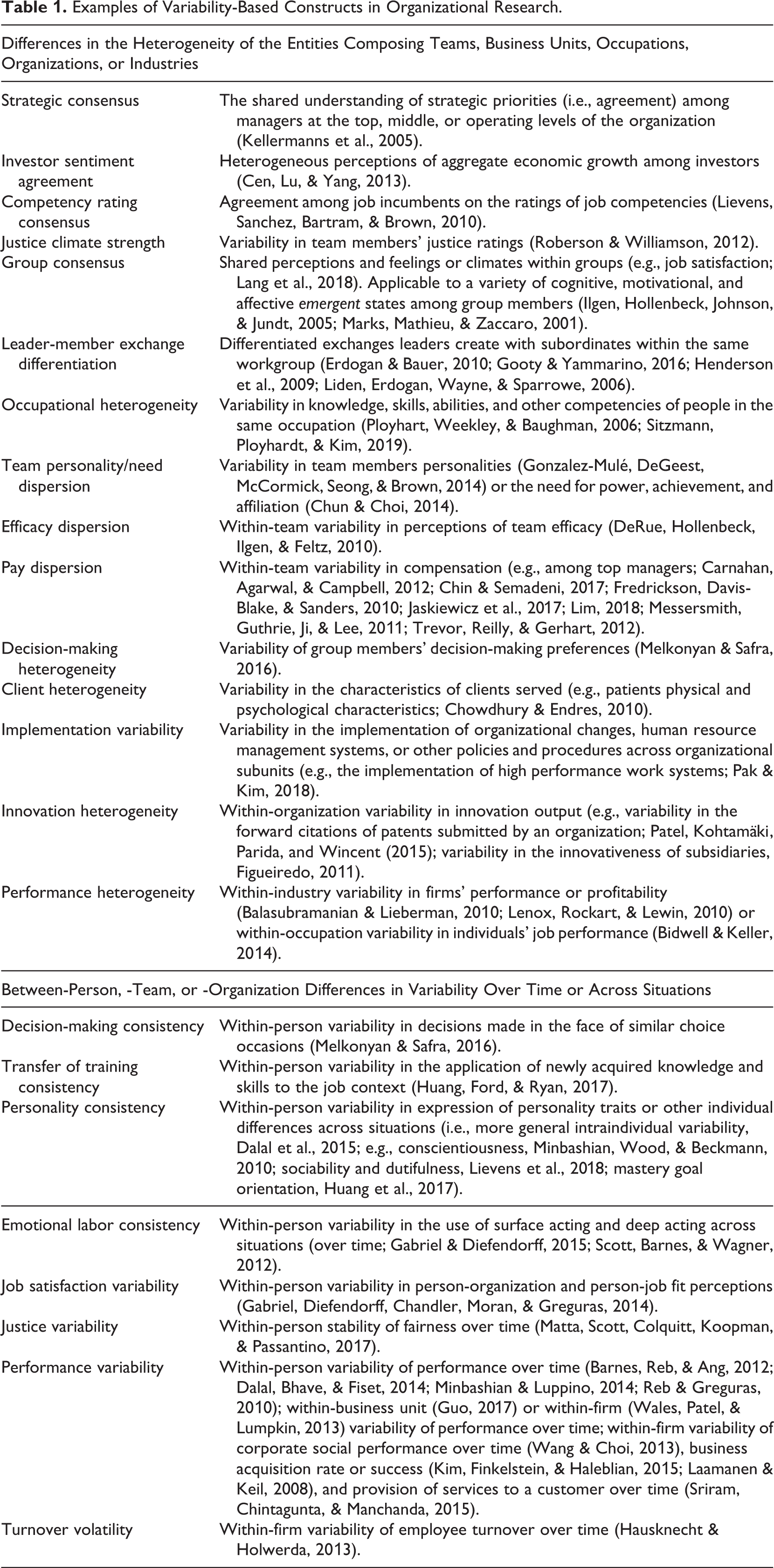
Across the micro-macro organizational research continuum, we identified many examples of variability-based constructs. These constructs reflect between-person, -team, or -organization differences in variability across time/situations (e.g., stability of preferences, attitudes, behaviors) as well as variability in the characteristics, perceptions, or behaviors of lower-level entities (e.g., people, but also teams, business units) that compose a higher-level entity (e.g., team, occupation, organization, or industry). Table 1 provides a description of these constructs.
Examples of Variability-Based Constructs in Organizational Research.
Many variability-based constructs have broad relevance across levels and areas of focus. For example, researchers have examined performance variability for firms over time (e.g., Wales, Patel, & Lumpkin, 2013; Wang & Choi, 2013), within an industry (e.g., Balasubramanian & Lieberman, 2010; Lenox, Rockart, & Lewin, 2010), across organizational subsidiaries (Figueiredo, 2011), across people who occupy the same type of job (Bidwell & Keller, 2014), and for employees over time (Barnes, Reb, & Ang, 2012; Reb & Greguras, 2010). Similarly, pay dispersion has been discussed in reference to labor markets (Cobb & Stevens, 2017), organizations as a whole (Carnahan, Agarwal, & Campbell, 2012), and perhaps most commonly, top management teams (e.g., Chin & Semadeni, 2017; Fredrickson, Davis-Blake, & Sanders, 2010; Jaskiewicz, Block, Miller, & Combs, 2017; Lim, 2018).
Several constructs also reflect variability in characteristics of group members (e.g., personality heterogeneity) or the extent to which there is agreement among members in the group (e.g., justice climate, efficacy dispersion). For example, strategic consensus regarding the firm’s priorities is commonly assessed for managers in the top team, but also at different levels and in different parts of the organization (Kellermanns, Walter, Lechner, & Floyd, 2005). The variability of supervisor behavior across time (e.g., justice variability; Matta, Scott, Colquitt, Koopman, & Passantino, 2017) and when interacting with different members of the workgroup (LMX differentiation; Gooty & Yammarino, 2016; Henderson, Liden, Glibkowski, & Chaudhry, 2009) has also been a topic of study.
It is important to note that most prior research has either conceptually discussed the nature of variance-based constructs or aimed to establish relationships between the construct and important workplace outcomes. For example, Ployhart, Weekley, and Baughman (2006) found that human capital emergence, conceptualized as consisting of both personality level (aggregate mean personality) and personality homogeneity (aggregate standard deviation of personality) within jobs and within organizations, predicted employee job satisfaction and performance. Further, research focusing on within-person personality consistency has found that the relationship between the level of personality traits and job performance is stronger when people are less variable in their personality expression across time/situations (Dalal et al., 2015). Other research has linked variability in the quality of relationships between a supervisor and his or her subordinates (i.e., LMX differentiation) to job satisfaction, performance, and other outcomes (e.g., Erdogan & Bauer, 2010; Schyns, 2006). In the literature on workplace groups and teams, researchers have proposed that team efficacy dispersion will predict team effectiveness above and beyond the average level of efficacy within the team (DeRue, Hollenbeck, Ilgen, & Feltz, 2010). At the department or organization level, researchers have found a stronger relationship between climate level (i.e., mean rating of perceptions of the workplace) and outcomes of interest (e.g., such as work satisfaction and organizational commitment) when employees view the climate similarly (i.e., there is a strong climate in place; González-Romá, Peiró, & Tordera, 2002). Finally, at the firm level, firms with higher trading variability have been found to have lower expected returns (Chordia, Subrahmanyam, & Anshuman, 2001).
These examples are part of the mounting evidence suggesting that variability (in addition to the average amount) of workplace phenomena predicts important workplace outcomes. Thus, there is a need to understand the antecedents of variability-based constructs. In the next section, we describe the smaller subset of studies (13) that have begun to examine these antecedents (see Table 2), including the limitations of approaches that have been applied previously. We explain how MELS and heterogeneous variance models address these limitations and expand the potential questions researchers may address when predicting variability as a substantive construct of interest.
Prior Organizational Research Predicting Variability-Based Constructs.

Use and Limitations of Aggregation Approaches for Predicting Differences in Variability
Our review found that researchers commonly calculate and use aggregate measures of variability as an outcome in single-level regressions or similar analyses. This approach has important limitations, which researchers can overcome by using multilevel approaches for predicting differences in variability.
First, this approach allows researchers to utilize only Level 2 predictors because Level 2 outcome variables (e.g., the standard deviation estimate most commonly used) do not have any Level 1 variability (Leckie et al., 2014). Thus, researchers cannot incorporate Level 1 variables as predictors of variability-based constructs and instead often create Level 2 versions of Level 1 predictors and utilize them in a single-level regression (Hofmann, 2002). This approach loses information that is likely of interest to researchers. In the sections that follow, we demonstrate how the ability to incorporate Level 1 predictors offers new avenues for organizational researchers.
Second, the aggregation approach does not account for uncertainty in the variability estimates. The standard deviation or variance of a sample is random. Therefore, there is uncertainty associated with that statistic. Further, the standard deviation of the variance (i.e.,
Explaining Sources of Variance Versus Predicting Heterogeneous Variances
The use of multilevel models for predicting the location (mean) is common across many areas in the organizational sciences. These models are often “mixed-effects” models because they include both fixed and random effects. For example, a random intercept multilevel model (i.e., the simplest multilevel model) is a “mixed” model that allows each Level 2 unit to have its own predicted mean (e.g., Bliese & Ployhart, 2002; Pinheiro & Bates, 2000). Adding fixed or random effects enable researchers to investigate change in mean-level based on either Level 1 or Level 2 characteristics. For example, it is common for researchers to employ growth models, such as those discussed by Bliese and Ployhart (2002), with data gathered using experience sampling methods in which participants respond to prompts on many occasions (Bolger & Laurenceau, 2013). When researchers use these models, the first step involves variance partitioning (i.e., quantify the amount of variability that exists at higher and lower levels of analysis) and then subsequently explaining some portion of the variance at each level (by predicting differential mean levels with variables of interest). The variance partitioning in these models is the same for everyone in the sample (e.g., one random intercept variance, one random slope variance, and one residual variance).
The characteristic that differentiates MELS and heterogeneous variance models from traditional multilevel models is the explicit modeling of variability (i.e., heterogeneous residual variances). The location side (mean portion) of the model is the same and can be expressed using the notation popularized by Raudenbush and Bryk (2002). The equation on the scale side (i.e., residual variability portion) takes a similar form but uses a different notation to make it easier to keep track of which side of the model the parameter is located. Thus, typical growth models (and other traditional multilevel models) are a special case of MELS and heterogeneous variance models where the scale side of the model contains only the fixed intercept, τ00. To clarify the difference between these types of models, see example equations for traditional regression, multilevel, heterogeneous variance, and MELS models provided in Figure 1 (compare Equation 2 for the traditional multilevel model to Equation 3 for the heterogeneous variance model and Equation 4 for the MELS model). Figures 2 and 3 further demonstrate this conceptual distinction between explaining sources of variance and predicting heterogeneous variances (i.e., differences in variability). The latter may be used to operationalize and predict variance-based constructs in the organizational literature.
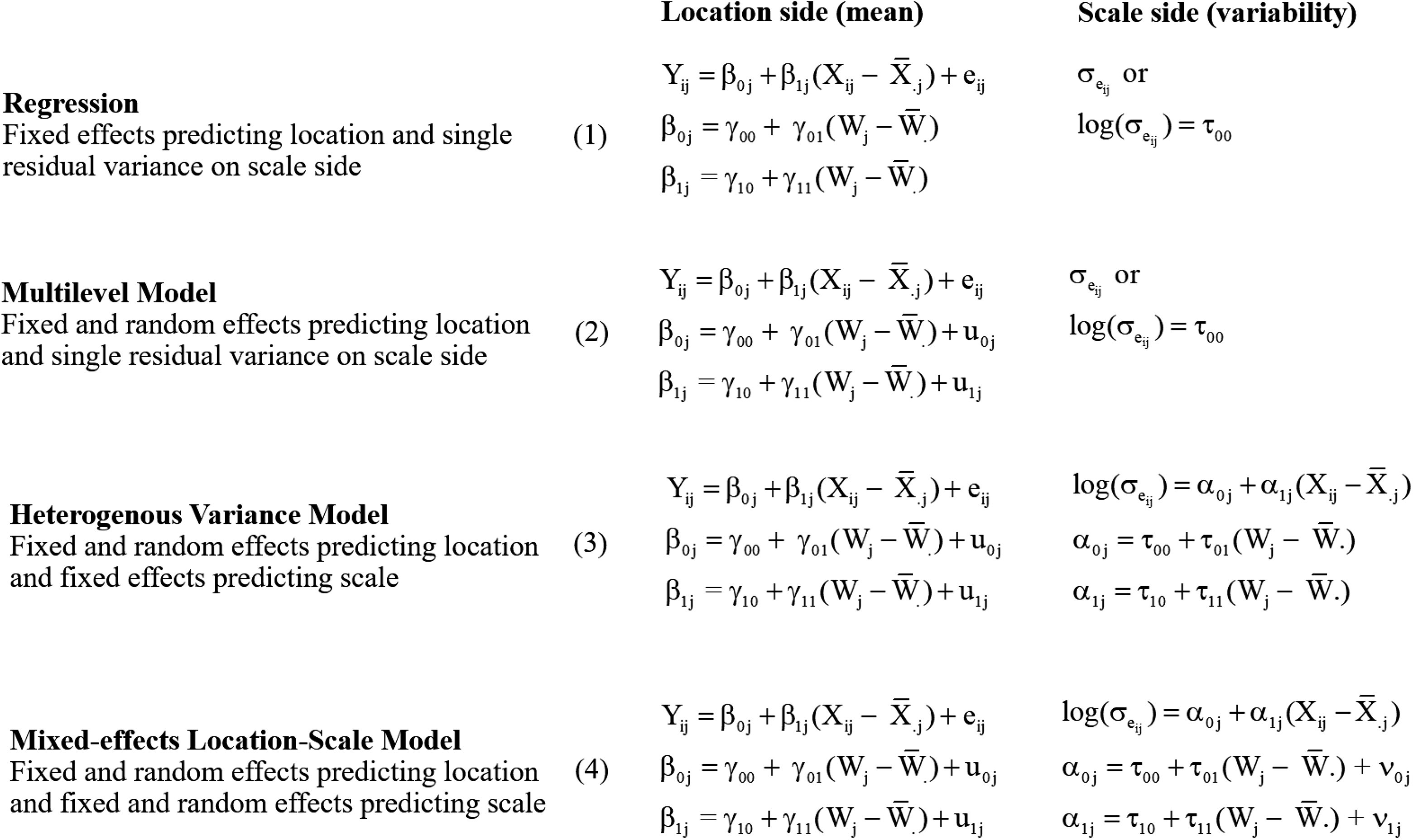
Comparison of regression, multilevel, heterogeneous variance, and mixed-effects location-scale model equations. The location or mean side of the regression equation is presented in a multilevel form, although it contains no additional random effects and is therefore not a multilevel model. This notation is used to facilitate the comparison of the equations across the various model specifications. Note that there is no Level 1 residual term on the scale side of the model (i.e., no e, which is similar to a generalized linear model [e.g., logistic regression] that also lacks a Level 1 residual). In MELS and heterogeneous variance models, the log of the variance (or standard deviation) is used as the outcome to ensure that the predicted variance is nonnegative.

Regression plot illustrating regression assumptions. The left panel contains a typical regression with a positive slope and a homogenous variance. Yi ∼ N(bxi, σ 2 ) is the common notation used to indicate that Yi is normally distributed with a mean that depends upon the individual’s xi value and a variance that is constant (σ 2 ). The right panel displays a heterogeneous variance model where the mean does not change over time depending upon x. The Yi ∼ N(0, τxi) notation indicates that the mean is zero for everyone in the sample and the variability depends upon the xi value.

Conceptual figure depicting predicted variances for two different groups in a MELS model. The black circles represent three different predictors (two at Level 2 and one at Level 1). The other circles represent the variance partitioning between Level 1 (white) and Level 2 (gray). The overlap between circles represents the variance explained. The size of the circle reflects group specific residual variance estimates. Group 2 has less random intercept variance (top circle) but more random slope (middle circle) and Level 1 (bottom circle) variance as compared to Group 1. In a traditional random slope multilevel model there are only three variance components for everyone in the entire sample. In other words, the size of the circles would be the same for all groups. Although not depicted here, the same principles apply to individuals.
Multilevel Models for Predicting Heterogeneous Variances
Above we discussed the conceptual differences between traditional multilevel models and multilevel models for predicting heterogeneous variances. In this section, we describe the notation presented in Figure 1 for the MELS model. In these descriptions, we use individuals nested within groups to make the interpretations more concrete. However, these interpretations would be similar for different nested cross-sectional and longitudinal designs. Also, please note that the interpretation for each coefficient is the same when the coefficients appear in the other more restricted models presented in Figure 1.
First, the location (mean) side of the model in Equation 4 (see Figure 1) is just like any other multilevel model:
Second, the scale (variability) side of the MELS model is a log-linear model in which the log of the residual variance or standard deviation (we use the standard deviation parameterization) is predicted by a linear function using predictors of interest. The log-linear model is used to ensure that the predicted standard deviation is positive. As shown on the scale side of Equation 4, each group (j) and individual within that group (i) has its own residual standard deviation estimate,
Finally, this model generally assumes all random effects ν’s and u’s are normally distributed with means of 0 and random effect standard deviations
If the scale side of the model contains fixed, but not random, effects of predictors (i.e., no ν0j or ν1j), then the model is considered to be a heterogeneous variance model. As described previously, heterogeneous variance models are a restricted version of the MELS model (compare Equation 3 to Equation 4 in Figure 1). This comparison is similar to how linear regression is a restricted version of multilevel models. Heterogeneous variance models, by their inclusion of only fixed effects on the scale side, predict variances that differ for systematic reasons (e.g., males are more variable than females). Recently, Lang et al. (2018) demonstrated the use of an extended multilevel model for heterogeneous variances to predict the emergence of within-group consensus over time. In their article, they estimated several models with random slopes on the location side and the fixed effect of time on the scale side. Some of these models included additional moderators of the effect of time on the scale side (e.g., leadership status and group readiness).
We build on this work by Lang and colleagues (2018) by demonstrating how random slopes may also be included on the scale side of the model. This extension is important because, in a different context, Leckie et al. (2014) and Walters et al. (2018) found that ignoring random effects on the scale side can lead to inflated Type I error rates when predicting heterogeneous within-group variances, specifically when testing hypotheses regarding Level 2 variables. Thus, heterogeneous variance models are susceptible to inflated Type I error rates if additional random effects are erroneously omitted. We want to emphasize that we are not saying the application of heterogeneous variance models is wrong, but rather using these models assumes a systematically varying cross-level interaction (i.e., the variances are heterogeneous due to time as well as other fixed effect interaction terms; Davidian & Giltinan, 1995; Hoffman, 2007; Raudenbush & Bryk, 2002). It is possible to test this assumption by examining the scale-model random effects in the more general MELS models.
A Bayesian Approach
Several years ago, Kruschke, Aguinis, and Joo (2012) outlined a case for the need to apply Bayesian methods in the organizational sciences (see Appendix B for a brief introduction to Bayesian statistics). Kruschke et al. recommend five steps researchers should follow when presenting the findings of a Bayesian analysis. We use these step-by-step guidelines as we make a case for the use of Bayesian methods to estimate MELS and heterogeneous variance models and present the results from our illustrative examples.
First, it is important for researchers to motivate the use of Bayesian methods. While researchers may estimate simple versions of multilevel models predicting heterogeneous variances using maximum likelihood estimation, convergence issues are likely to occur as the number of random effects increase on the location and scale sides of the model (Asparouhov & Muthén, 2016). Thus, we use Bayesian analysis to “open the door to extensive new realms of modeling possibilities that were previously inaccessible” (Kruschke et al., 2012, p. 723). In other words, Bayesian approaches allow researchers to estimate complex models that would be extremely difficult if not impossible to estimate using frequentist approaches (e.g., MELS models that have random intercepts and slopes on both the location and scale sides of the model).
Second, researchers should describe the model and its parameters in detail. We provide this information for both of our illustrative examples in Appendices D and E as well as in the supplemental material. Third, researchers should justify the use of the prior in their analysis. The priors we used were intended to be uninformed (i.e., should not affect the
Fourth, Kruschke et al. (2012) encouraged researchers to describe the Markov chain Monte Carlo (MCMC) process in detail (see Appendix C). The models are estimated using Stan (Carpenter et al., 2017) through the brms R package (Bürkner, 2017). Stan is a powerful probabilistic programming language that allows researchers to estimate many different types of complex models. The Stan programming language is similar to other open-source Bayesian software like OpenBUGS (Spiegelhalter, Thomas, Best, & Lunn, 2007) or JAGS (Plummer, 2013). However, working with the Stan code directly is more difficult than working with these other software programs or typical R packages. The brms package was written to reduce this burden (Bürkner, 2017) and may be used by researchers to generate efficient Stan code. The brms package requests that you provide code that is similar to typical multilevel model code in R (e.g., see the lme4 R package; Bates, Maechler, Bolker, & Walker, 2015). The brms code is then translated into the Stan language (i.e., brms creates the Stan code as well as the Stan data file).
Estimating a Bayesian MELS or heterogeneous variance model in Stan offers, at least, two important advantages over frequentist approaches. First, these models can partition the variability multiple times on both the location and the scale side of the model. Thus, inevitably, some of the variance components are going to become small and likely inestimable using a frequentist framework (Asparouhov & Muthén, 2016). As mentioned previously, a Bayesian approach allows researchers to estimate models with small variance components. Second, Stan uses a different sort of Bayesian sampling procedure (i.e.,
In addition to describing this estimation procedure, researchers should provide evidence that the sampler has converged and adequately sampled throughout the posterior distribution (Kruschke et al., 2012). For each example, we provide evidence that the different starting values (i.e., different
Illustrative Examples
In this section, we provide illustrative examples for nested cross-sectional and longitudinal designs. These examples utilize simulated data (see Appendix D for details regarding data generation) to demonstrate the sorts of research questions that can be addressed using MELS and heterogeneous variance models. Given that the purpose of this article is to demonstrate the flexibility of these methods, the illustrative examples involve relatively complex models that incorporate random slopes. In Appendix E, we provide model alternatives that gradually increase in complexity from an empty linear regression model to a MELS model with random slopes on both sides of the model. These buildup analyses are presented using general notation (i.e., not in the context of the illustrative examples). In the remainder of this section, we briefly describe illustrative research questions and then present the analysis and results as would be typical in a published empirical study. In the supplemental material, we provide the code needed to generate the data that serve as the basis for our illustrative examples as well as the code needed to analyze these data. We also provide interpretations of all parameter estimates (see “Readme.doc” for the intended use of each file). The level of detail provided in the supplemental material would not typically be provided in published articles; this information is meant to aid researchers as they move from output interpretation to writing up the results of their own study.
Nested Cross-Sectional Example: LMX Differentiation
This first example illustrates how the MELS model can be used with nested cross-sectional data to provide new insights into the nature of leader membership exchange (LMX) differentiation. It is common for supervisors to develop different quality relationships with the subordinates they supervise (i.e., who are nested within the leader’s group) resulting in a pattern of LMX that can be described by central tendency (e.g., the mean), variation (e.g., the standard deviation), and relative position (i.e., how does an individual’s LMX compare to others with the same leader; Martin, Thomas, Legood, & Dello Russo, 2018). The MELS model allows researchers to predict these three properties in a single model, while appropriately considering model uncertainty and avoiding the use of aggregation and its associated problems. In this illustrative example, we consider the effects of transformational leadership (i.e., a Level 2 predictor) and a leader’s perceived similarity with each subordinate (i.e., a Level 1 predictor) on LMX reported by subordinates.
Previous research has found that perceived similarity is predictive of higher-quality LMX relationships (Liden, Wayne, & Stilwell, 1993). As a Level 1 variable, perceived similarity can have between, within (relative), and contextual effects (Enders & Tofighi, 2007; Kreft, De Leeuw, & Aiken, 1995) on either the location or the scale side of the model. 2 The within-group level of the model (i.e., Level 1 or subordinate level), which applies to both the location side and the scale side of the model, predicts the relative position piece of the LMX outcomes (see Equation D1 in Appendix D). In this example, γ10 denotes the relative similarity effect on the location side of the model, and τ10 denotes the same effect on the scale side.
Henderson et al. (2009) proposed that transformational leadership may combine with perceived similarity to predict LMX differentiation. They suggest that more transformational leaders (e.g., Leader A in Figure 4) will be less affected by perceived relative similarity. Specifically, we expect that more transformational leaders will have higher mean LMX ratings and that their LMX ratings will be less variable regardless of perceived similarity. In contrast, we hypothesize that less transformational leaders will have lower mean LMX and that their ratings will be more variable (i.e., see differentiation or distance between the data and line for the subordinates who report to Leader B in Figure 4). For these leaders, relative similarity will be more likely to affect relative LMX ratings in terms of the predicted mean LMX as well as in terms of the variation around that predicted mean. Leaders low on transformational leadership will have higher and more consistent LMX with similar group members. These effects manifest themselves in Figure 4 for Leader B as a positive slope of relative similarity on relative LMX and a shrinking distance between the x symbols and the predicted mean (demarked by the line) as similarity increases. We examine these assertions in our illustrative analysis.

Depiction of hypothetical leaders who differ in transformational leadership. The two lines depicted in this figure represent different leaders (A & B). The location of the subordinates (depicted by o) around Leader A’s line (who is high in transformational leadership) indicates that this leader has high and consistent leader-member exchange (LMX) relationships with subordinates regardless of the level of similarity between the leader and the subordinate. Consistency is indicated by the equal distance of the o symbols from the line. The location of the subordinates (depicted by x) around Leader B’s line (who is low in transformational leadership) indicates that LMX for this leader depends upon similarity such that the leader has higher LMX with subordinates who are more similar to the leader. Further, the distance of the xs from the line indicates that subordinates who are more similar to the leader are treated more consistently.
Analysis and Results
Prior Justification
To assess the sensitivity of the inferences to the prior, we utilized multiple sets of priors (i.e., two noninformative or vague options and one informed option). The results did not vary greatly. Thus, we present the results using the default uninformed priors. We provide the specific priors used in these analyses below and refer readers to McElreath (2016) and Bürkner (2017) for more information regarding the choice of priors. One advantage of using brms with uninformed priors is that the user does not have to specify the priors. As a default, priors designed not to influence the final results are incorporated into the analysis. In the supplemental material, we illustrate that in less complex models where both the frequentist and Bayesian models are estimated, the results match to two or three decimal places when using similar priors. Thus, these priors are not affecting the final results. In this analysis,
Model Convergence
Before interpreting the results from the MCMC process, we assessed whether the sampler converged and adequately sampled throughout the posterior distribution. If this is not the case, then the results cannot be interpreted. Two potential problems that could prohibit reaching these goals are
Random and Fixed Effect Output for the Nested Cross-Sectional Leader-Member Exchange Differentiation Example.
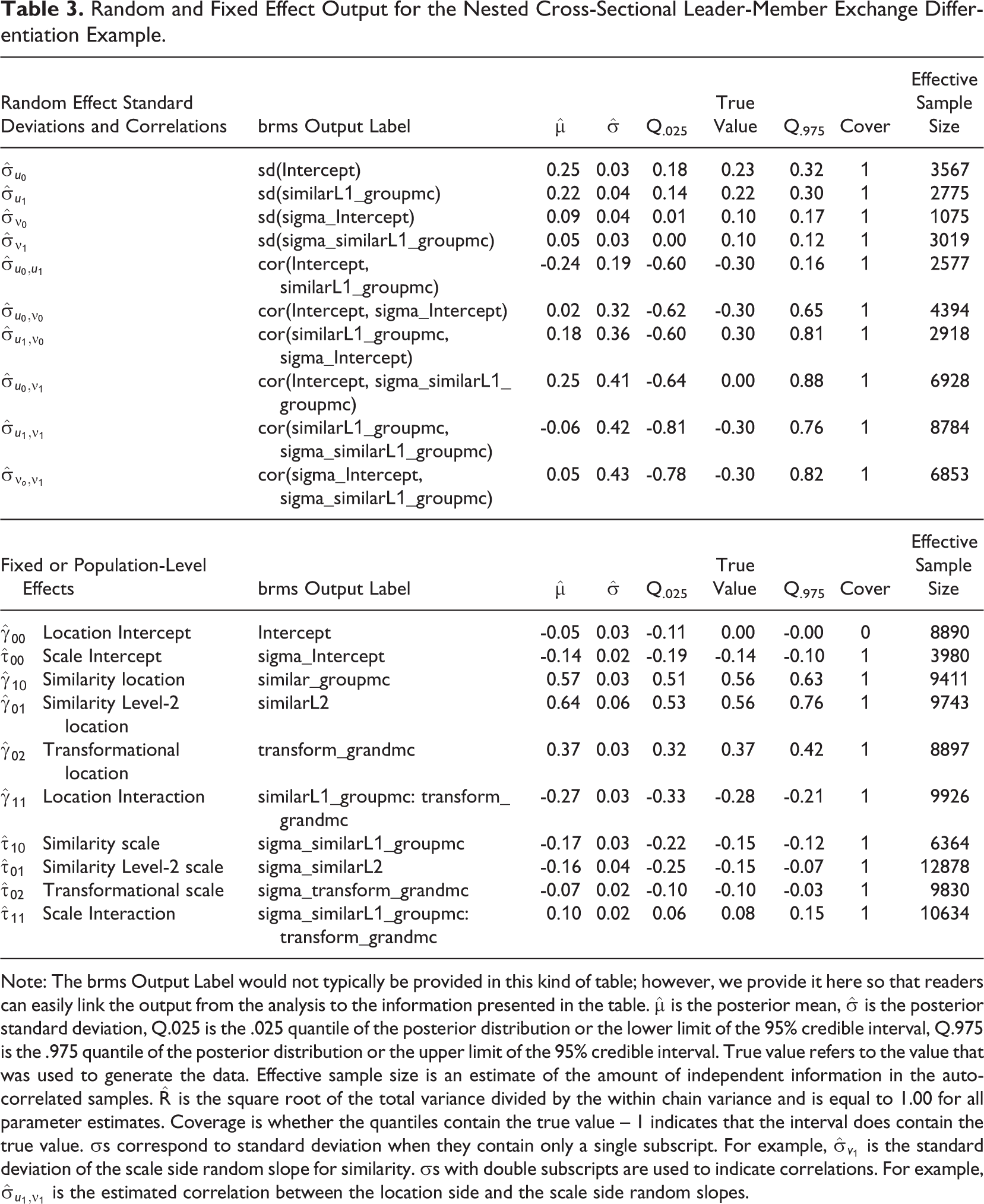
Note: The brms Output Label would not typically be provided in this kind of table; however, we provide it here so that readers can easily link the output from the analysis to the information presented in the table.
To assess whether autocorrelation is prohibiting adequate sampling from the entire posterior distribution, we investigated two sources of information (i.e., trace plots and the
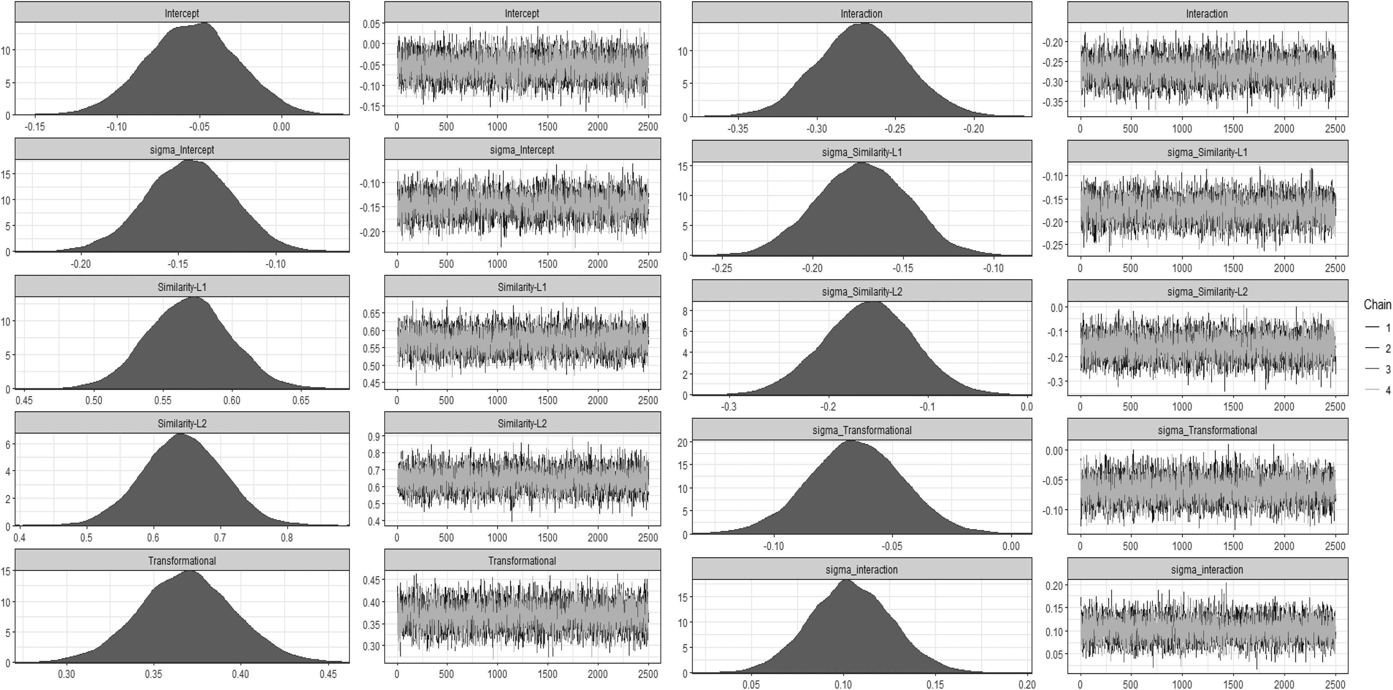
Density and trace plot for the Markov chain Monte Carlo samples for the nested cross-sectional leader-member exchange differentiation example.
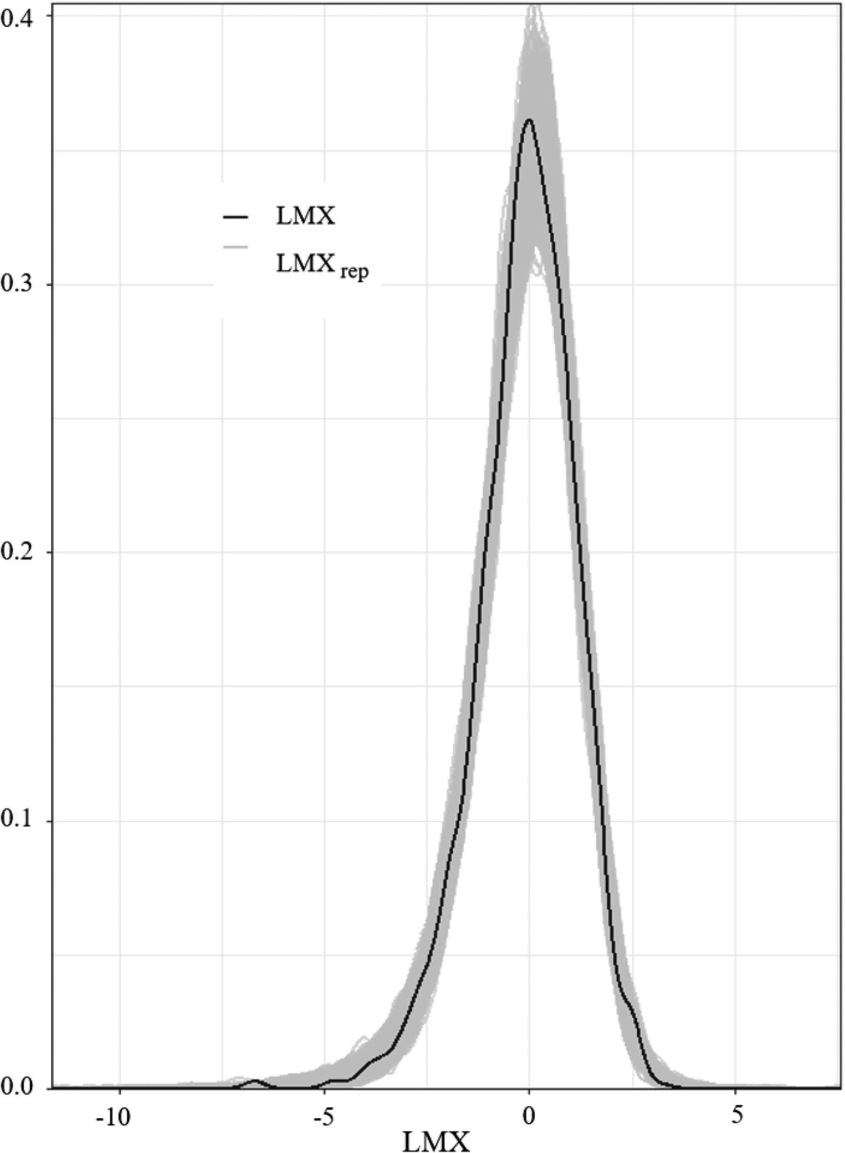
Posterior predictive plot for the nested cross-sectional leader-member exchange differentiation example. The observed data are in black, and the data generated from the model are in gray.
The final indication that the model is performing as expected is only available because we simulated the data. The credible intervals contained the data-generating parameters for all the parameters except for the location intercept. Thus, the 95% credible intervals contained the data-generating (true) value for 19 of the 20 estimated parameters (i.e., 95%). Also note that the model was able to detect all nonzero fixed effects and the nonzero random effect standard deviations; the ability to detect nonzero effects is important, because having credible intervals that contain all parameters may be an indication that the intervals are too wide. This does not appear to be the case. However, there were some effects that the model did not detect; none of the nonzero correlations between the scale model random effects were significant. Thus, a larger sample size is needed to detect these correlations.
Interpretation of Posterior Distribution
Both the mean and the variance sides of the model contain the similarity-by-transformational leadership cross-level interaction, the associated simple main effects, and the Level 2 similarity effect. The location intercept
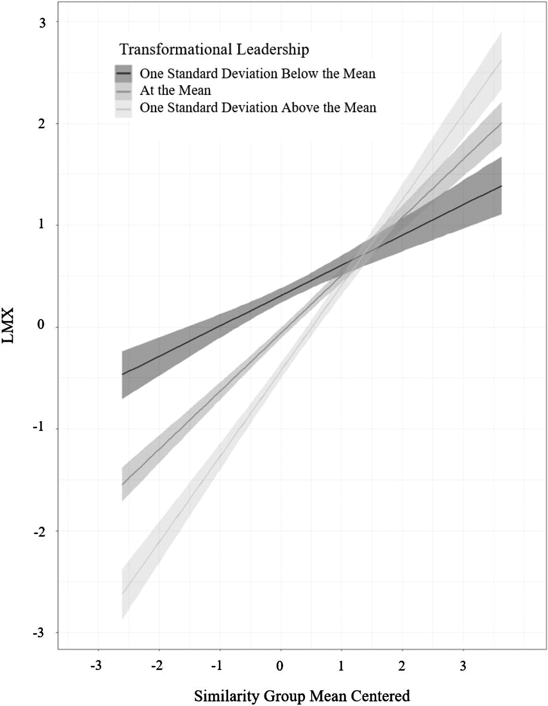
Cross-level interaction plot demonstrating how transformational leadership moderates the effect of similarity on leader-member exchange for the location side of the model (i.e., the predicted mean). The bands reflect the 95% confidence interval.
The scale side of the model is interpreted similarly. The scale intercept,

Cross-level interaction plot demonstrating how transformational leadership moderates the effect of similarity on leader-member exchange for the scale side of the model. This plot presents the results for the log residual standard deviation.
In addition to interpreting the scale side of the model on the log metric, the model can also be interpreted in terms of standard deviations (Lang et al., 2018). These standard deviations are the predicted residual standard deviation (i.e., square root of the residual variance) given specific predictor values. Computing the predicted standard deviation is performed by exponentiating the coefficients; the standard deviations can then be converted into a percentage change that provides a meaningful effect size metric. See Appendix F for a more detailed explanation for this calculation. For example, assuming average similarity (i.e., both the Level 2 and Level 1 predictor values are zero) the predicted standard deviation for a group with a leader that is one unit above average on transformational leadership is calculated as e(–.14 – .07). Thus, their predicted standard deviation value is approximately .81. If the leader had an average level of transformational leadership, then the predicted value would be e-.14, which is approximately .87. The percentage change is computed as (.81 – .87)/.87, which is approximately –.07 or a 7% decrease. Thus, for a one-unit increase in transformational leadership the standard deviation of LMX is reduced by seven percent.
A similar interpretation could be made for the similarity effect for those in a group with a leader that has an average level of transformational leadership and an average group similarity. A one-unit increase in perceived similarity results in a [(e–.14 – .17 – e–.14)/e–.14] × 100 = −15.63% decrease in the predicted standard deviation of LMX. The percentage change is smaller for more transformational leaders. Further, Figures 8 and 9 demonstrate how the slope for similarity as a predictor becomes smaller as transformational leadership increases.

Cross-level interaction plot demonstrating how transformational leadership moderates the effect of similarity on leader-member exchange for the scale side of the model. This plot is rescaled to represent the residual standard deviation.
In summary, LMX relationship quality is affected less by perceived similarity when leaders are higher in transformational leadership. In terms of central tendency, a positive simple main effect of relative similarity (i.e., γ10) indicates that those with relatively more similarity are expected to have higher mean levels of LMX, but that effect decreases as transformational leadership increases. In terms of variation, relatively high similarity results in more consistent LMX relationships. This effect decreases as transformational leadership increases, indicating that transformational leaders treat subordinates consistently regardless of similarity. Groups with similar members have higher mean levels of LMX and less differentiation in LMX ratings.
Longitudinal Example: Between Firm Performance Variability
This second example illustrates how a heterogeneous variance model could be used with longitudinal data to provide new insights into between-firm performance variability differences based on the strategy enacted by different firms. Imitation has traditionally been assumed to reduce between firm performance heterogeneity in an industry. However, Posen and Martignoni (2018) challenged that assumption with a computational model that illustrates the conditions in which imitation can increase between firm performance heterogeneity. They theorize that due to limited information, imitating firms will be unable to duplicate the desired strategy completely and obtain the desired performance. Instead, “copying” firms will have to engage in post-imitation learning where the initial imitation strategy is adjusted. Firms may vary widely in their post-imitation learning ability. Thus, imitation results in both an increased likelihood of achieving the desired performance and an increased likelihood of performing far worse. Thus, there will be increased between-firm performance variability overtime when firms in an industry adopt an imitation strategy.
The data generated in this hypothetical example are meant to emulate monthly performance data across a fiscal year (see Appendix D for details). Thus, time is nested within firm, and each firm is measured on 12 equally spaced occasions. We compare an “imitator” set of firms to a “business as usual” set of firms (i.e., those that continue to perform their preexisting strategies). The outcome is defined generically as firm performance. In terms of heterogeneous variance models, this specific model contains a cross-level interaction on the location side (i.e., the same model as seen in the nested cross-sectional example) and a heterogeneous pattern of Level 2 covariance matrices (i.e., covariance matrices that are systematically varying due to the strategy adopted). The easiest way to estimate this model that allows us to use brms (instead of utilizing Stan directly) is to employ a multiple group approach where each group (i.e., imitators versus business as usual) is allowed to have its own covariance matrix. This approach is similar to some of the approaches described by Kuppens and Yzerbyt (2014). As previously stated, there is a random intercept and linear slope for time as well as their covariance on the location side of the model. In other words, the model allows for differences in terms of initial firm performance (i.e., at the beginning of the fiscal year) and also differences in terms of how much they grow from month to month. The heterogeneous between-group covariance matrices are based on the following rationale.
The decision to imitate the industry leader may be a radical change from the existing practices, and the decision-makers in a firm are likely to be resistant to such radical forms of change. This drastic step would not be taken unless the firm is performing poorly. Based on this rationale, at the beginning of the fiscal year, the imitating firms are hypothesized to have consistent poor performance (i.e., a smaller between-group variability). The location slope variability is hypothesized to be larger in the imitating firms for reasons described previously. Finally, the correlation (i.e., standardized covariance) between the intercept and slope is generated to be larger in the imitation group than the business as usual group. This hypothesis is based on the rationale that very poor initial performance is expected to be associated with a lack of resources or ability to compete in the industry. In other words, no matter what sort of strategy they choose, they are unlikely to succeed.
Analysis and Results
Prior Justification
As in the first illustrative example, the analysis model is the same as the data-generating model, and we use noninformative default priors. The default noninformative priors for the fixed effects are improper (i.e., the distribution does not integrate to one) flat priors (Bürkner, 2017). The standard deviations of the random effects in brms have a default prior of a half student-t distribution with 3 degrees of freedom and a location and scale parameter of 0 and 10 respectively. The prior for each of the 2 × 2 correlation matrices is the LKJcorr (1) (Lewandowski et al., 2009), which is a flat prior over all valid correlation matrices.
Model Convergence
The convergence diagnostics of

Density and trace plot for the Markov chain Monte Carlo samples for the longitudinal between firm performance variability example.
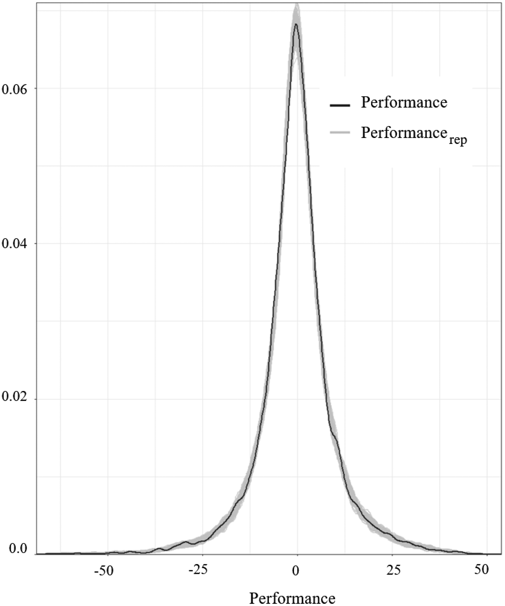
Posterior predictive plot for the longitudinal between firm performance variability example. Note that the observed data are in black and the data generated from the model are in gray.
Fixed and Random Effect Output for Longitudinal Between Firm Performance Variability Example.
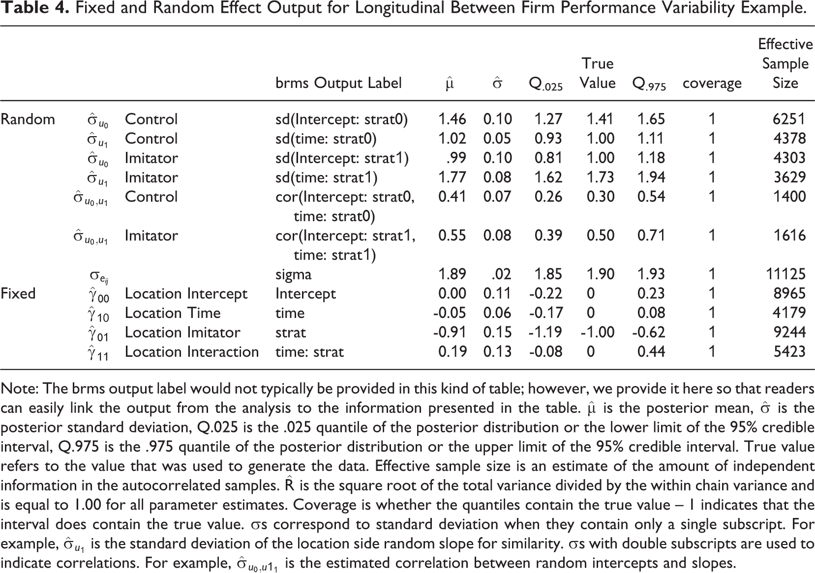
Note: The brms output label would not typically be provided in this kind of table; however, we provide it here so that readers can easily link the output from the analysis to the information presented in the table.
Interpretation of Posterior Distribution
The interpretation for the location side of the model is the same as a typical multilevel model with a cross-level interaction. The only nonzero effect in this example was the simple main effect of being an imitator. In line with the first, hypothesis, at the beginning of the study, the imitators are predicted to perform worse than the business as usual condition,

Cross-level interaction plot demonstrating how strategy moderates the change in average performance over time. The shaded regions or bands reflect the 95% confidence interval.
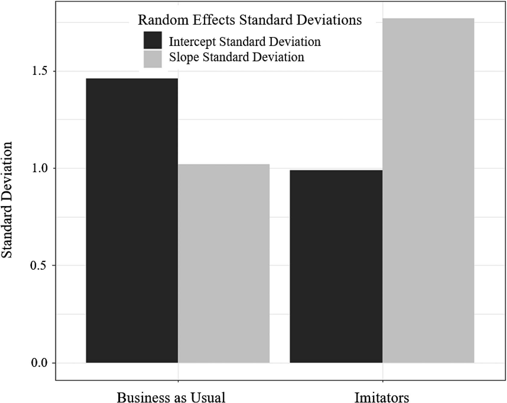
Bar chart displaying random intercept and slope standard deviations by strategy.
Variability Magnitude Hypotheses.
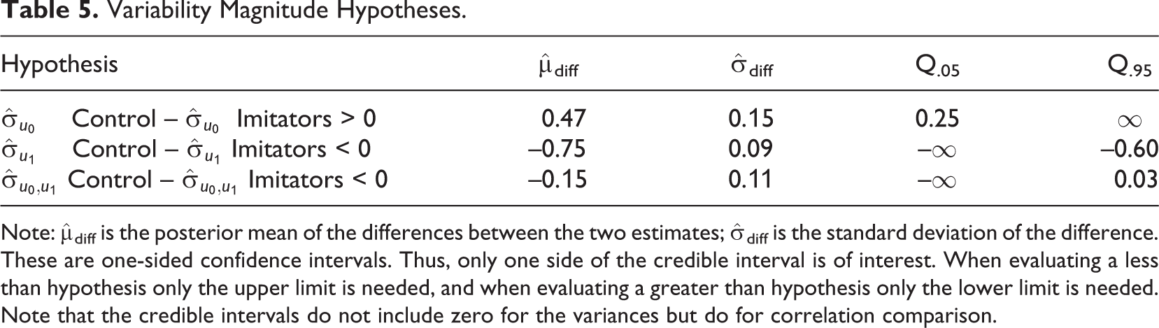
Note:
Discussion
Interest in predicting variance-based constructs is increasing among organizational researchers. Lang et al. (2018) recently illustrated the use of a multilevel model to predict changes in consensus (agreement) among members of a group over time. We build upon this first application of multilevel models for predicting heterogeneous residual variances in the organizational sciences by highlighting the flexible nature of MELS and heterogeneous variance models. Researchers can utilize these models in both micro and macro organizational research with different designs (nested cross-sectional or longitudinal) to model different portions of the variability (within- or between-group variability). Below we summarize the advantages of using the most general MELS models.
Advantages of Using MELS
The MELS model offers several statistical advantages over other approaches, including heterogeneous variance models. First, by including random effects (particularly the random intercept on the scale side of the model), it is possible for researchers to test the assumption that all Level 2 units have the same amount of within-group/person variability (i.e., homogeneous variances) and avoid inflated Type I error rates (Leckie et al., 2014; Walters et al., 2018). Moreover, this model allows researchers to avoid the limitations of aggregation (i.e., computing a standard deviation for each group and predicting it in a single level regression) that include the inability to include Level 1 predictors and disregarding uncertainty in the aggregated variability estimates. This uncertainty should be and is accounted for when the data are analyzed with the MELS model.
As mentioned previously, applying MELS models to predict a construct of substantive interest increases the types of research questions that researchers can address. To this point, organizational researchers have predominately focused on hypotheses about the amount (mean) of responses. However, researchers should consider whether there are sound theoretical reasons to propose hypotheses aimed at predicting variability. Our illustrative example using nested cross-sectional LMX data exemplifies the types of questions that can be addressed with multilevel models but are not possible to examine using an aggregation approach. In the example, cross-level interaction research questions with random slopes for both the mean and the residual standard deviation were addressed using data that were generated based upon a substantive example. In the context of LMX and LMX differentiation, perceived similarity was allowed to have random slopes when predicting LMX mean (location) and LMX differentiation (scale); perceived similarity was also allowed to have Level 2 effects on both sides of the model. The effect of perceived similarity was qualified by transformational leadership as a moderator.
Researchers may also examine questions that consider the amount (mean) and the variability in combination. For example, researchers studying the results of an intervention may find that a particular treatment not only increases the mean of a construct (e.g., employee wellbeing) but also decreases the variability of ratings over time. As another example, researchers might propose that the intervention treatment group would start with a mix (high variability) in wellbeing scores, but over time, all individuals in the treatment group would both improve and become more homogenous. In contrast, a less advantageous treatment might increase the mean, but may also increase the variability. In this case, although on average wellbeing may be improving, the results also suggest that the treatment is creating a disparity between people. In other words, the treatment works for some but not for others. This finding would be similar to the results of the second illustrative example examining firm performance. The ability to predict the mean and variability in the same model makes it possible to test these sorts of combination hypotheses.
Practical Recommendations
Bayesian estimation is appropriate and likely necessary when estimating complex MELS models because of the large number of random effects. The Bayesian approach, in conjunction with brms (Bürkner, 2017) and Stan (Carpenter et al., 2017), utilized in this article allows for the estimation of random slopes as well as cross-level interactions in both sides of the model. In terms of software comparison, brms and Stan is the most widely available alternative. The only other software that has been utilized to estimate this model is Stat-JR which is also a Bayesian program that is distributed with MLWin (Browne, 2017). MixRegLs (Hedeker & Nordgren, 2013) or MixWild does not allow for random slopes on the scale side, and as of version 8.0, Mplus (Muthén & Muthén, 1998-2017) can specify heterogeneous variances, but it is unclear how a random slope could be incorporated on the scale side. Perhaps, the dynamic structural equation modeling framework (Asparouhov, Hamaker, & Muthén, 2018) that incorporates time series analysis into a structural equation modeling framework could provide an alternative.
Bayesian analyses offer several statistical advantages; however, these approaches are also unfamiliar to many researchers. Providing priors is an extra step in conducting an analysis, and researchers must ensure that their choices regarding priors do not influence the final result inappropriately. While brms helps reduce the burden on researchers by supplying default priors that seek not to influence the final results, this is still an issue that researchers should consider. Convergence issues can occur in Bayesian analysis, and when they do, researchers must resolve these issues by investigating various convergence diagnostics. Particularly, researchers may face challenges when estimating random slopes on both sides of the model. We provide code to perform the analyses but do not provide a lengthy discussion of the process of addressing convergence issues. We encourage researchers to consult accessible resources, including Kruschke (2015) and McElreath (2016), as this process is very data/model dependent.
To demonstrate the flexibility provided by utilizing a Bayesian approach to testing variability-related hypotheses, we present a complex MELS model (i.e., with random slopes on the location and scale sides). However, in some cases, less complex models may be more aligned with the questions of substantive interest. We recommend readers use Appendix E as a tool to consider the different types of models they may estimate and to pick the model that best fits their theory and research questions.
One very important takeaway from our review of the existing literature is that precise language is necessary when interpreting complex multilevel models. We found instances where researchers were conducting traditional multilevel models (e.g., growth models) and interpreting the results as if they were predicting heterogeneous variances. Language such as “we predicted variability” may lead readers to think that the study is predicting heterogeneous residual variances when the study is actually using a traditional multilevel model to explain a portion of a single variance estimate that the model provides for everyone in the study (e.g., a Level 2 predictor explains some random intercept variance; see Figure 3). Thus, we recommend that researchers use more precise language when describing their analysis. For example, researchers applying these models should clarify that they used a MELS or heterogeneous variance model to predict heterogeneous residual variances. This language should make it clear that the outcome of interest is a variance-based construct and that these analyses are distinct from explaining variability as is done in a typical regression analysis.
Researchers may have questions regarding centering decisions in MELS and heterogeneous variance models. To our knowledge, researchers have not examined this issue with these specific models. However, given that the scale- side of the model is a log-linear model, researchers may interpret the τs as they would the βs on the scale side. Enders and Tofighi (2007) advise that centering decisions should be based on the research question of interest. Researchers who are interested in Level 1 predictors could include the group mean centered version of the Level 1 predictor without including the Level 2 variable. However, if this approach is used, it is important to remember that all Level 2 variability is being ignored. When researchers are interested in both Level 1 and Level 2 versions of the same predictor, then either group or grand mean centering can be used to provide the Level 1, the Level 2, and the contextual effect. Either approach will provide two of these three effects, and the third effect can be calculated from the other two (Enders & Tofighi, 2007). Further, for researchers interested in a Level 2 predictor only, centering decisions are not overly complicated, and advice concerning single-level regression analyses applies.
Researchers may be interested in providing effect size calculations for models with random slopes on the scale side. Pseudo-R2 values could be calculated for each of the variance components in this model, and they have been shown to work well with models that include random intercepts on both the location side and the scale side (Walters et al., 2018). However, these analyses have yet to be extended to the random slope case. Until this research is conducted, researchers may consider using the intuitive effect size estimate obtained by calculating the proportional increase/decrease in the standard deviation (Lang et al., 2018).
Researchers should be aware that a mediation version of the MELS model has also not yet been developed and evaluated. Many of the hypotheses discussed in this article could easily be expanded to include mediated relationships. For example, the LMX example could be extended to view LMX differentiation as a mediator and add group performance as the distal outcome (Henderson et al., 2009). To address this hypothesis without the shortcomings of aggregation, a mediation version of the model would need to be developed.
Power analyses have also not yet been conducted for the full MELS model presented in this article (i.e., random slopes on both sides of the model). However, recent research examining less complicated models has begun to provide some insight into power issues with these analyses. For example, Walters et al. (2018) found that the power to detect the scale-model random intercept variance and the effect of an individual-level predictor of residual variability increased with the number of individuals and occasions of measurement (and provided power curves that may help researchers planning to conduct a similar analysis).
Research on longitudinal modeling has demonstrated the benefits of model building that occurs in a step-up fashion where the models start simple and become increasingly complex. For example, polynomials of increasing order are often fit to get the best model for improvement over time before adding any additional predictors to the model. Within a given side of the model, it makes sense to model the effect of time correctly before adding in any additional predictors. However, whether researchers should model the location (mean) or scale (variance) side of the model first remains an open question or future research. As methodological work on these models proceeds, researchers should ground their modeling building in theoretical arguments and also test multiple competing models. These models can be compared using the Watanabe-Akaike information criterion (WAIC; Gelman, Hwang, & Vehtari, 2014) which is an extension to the commonly applied Akaike information criterion (AIC; Akaike, 1998) that does not assume that posterior distribution is approximately multivariate normal. We provide examples illustrating how to conduct model comparisons in the supplemental material.
Conclusion
Variability is no longer viewed as something to be averaged over, ignored, or tricked into fitting the assumptions of a typical general linear model. It is substantively interesting to researchers working in many different areas. Regression models produce normal distributions that are conditional on the values of the predictors and their associated regression coefficients. Like any normal distribution, these distributions are characterized by both the mean and the variance. Thus, every effort that is used to model the mean correctly should be used to model the variability correctly as well. By expanding the multilevel repertoire to include MELS and heterogeneous variance models, researchers can appropriately analyze mean and variability-related hypotheses at multiple levels simultaneously.
Footnotes
Appendix A
Appendix B
Appendix C
Appendix D
Appendix E
Appendix F
Authors’ Note
We would like to thank Justin Jones as well as special feature editor Rory Eckardt, the other editors, and anonymous reviewers for the Feature Topic on New Approaches to Multilevel Methods and Statistics for their comments and suggestions throughout the review of this article.
Houston F. Lester is also affiliated with Center for Innovations in Quality, Effectiveness and Safety, Michael E. DeBakey VA Medical Center, Houston, Texas.
Declaration of Conflicting Interests
The author(s) declared no potential conflicts of interest with respect to the research, authorship, and/or publication of this article.
Funding
The authors disclosed receipt of the following financial support for the research, authorship, and/or publication of this article: This work was partially funded by the first author’s VA Health Services Research & Development (HSR&D) Postdoctoral Fellowship: HX-17-014.