Comparing Churn Prediction Techniques and Assessing Their Performance

Abstract

Customer retention has become a focal priority. However, the process of implementing an effective retention campaign is complex and dependent on firms’ ability to accurately identify both at-risk customers and those worth retaining. Drawing on empirical and simulated data from two online retailers, we evaluate the performance of several parametric and nonparametric churn prediction techniques, in order to identify the optimal modeling approach, dependent on context. Results show that under most circumstances (i.e., varying sample sizes, purchase frequencies, and churn ratios), the boosting technique, a nonparametric method, delivers superior predictability. Furthermore, in cases/contexts where churn is more rare, logistic regression prevails. Finally, where the size of the customer base is very small, parametric probability models outperform other techniques.

Keywords

customer churn prediction profitability retention probability models data mining simulations

Introduction

Today’s intense competition has forced companies to focus more attention and resources on customer retention (Roos and Gustafsson 2007). This has also been reflected in an industry report, which found that the majority of Chief Marketing Officer (CMOs) consider retention to be their top priority, allocating the largest share of their budgets to it (Forbes 2011). Although the idea of convincing defecting customers to stay is intuitively appealing, it is not straightforward in practice.

The main focus of customer retention is the prevention of customer churn (Bijmolt et al. 2010). However, convincing customers to stay by any means should not be the ultimate goal. Only profitable would-be churners should be encouraged to stay, while unprofitable customers should be allowed to defect (Reinartz and Kumar 2003). One of the ways to prevent customer defection is to be proactive and provide would-be churners with appropriate incentives before it is too late (Neslin et al. 2006).

Previous research has focused on profitable customers and indicators of when they might become unprofitable. Reinartz and Kumar (2003) applied the customer lifetime value (CLV) concept to inform the decision as to when to stop pursuing a customer(s). In other words, unprofitable customers were simply excluded from further analysis. However, should firms just let these customers go or should they attempt to retain them? If so, which customers are worth retaining? We address these important questions.

As a point of departure, we use the concept of profitable lifetime duration as proposed by Reinartz and Kumar (2003). Specifically, in the context of catalog retailing, they suggest computing the net present value of expected contribution margin of customers and comparing it with the cost of mailing. If the latter is larger, then the relationship with the customer is terminated. Although this approach gives a simple answer to the relationship termination question, it ignores the fact that termination may in fact not be the optimal decision, particularly when certain customers may be amenable to the sorts of retention strategies suggested in this article.

Another question that challenges Reinartz and Kumar’s (2003) approach is the computation of customers’ probability of being active. While their study employs a gamma-exponential/negative binomial distribution (Pareto/NBD) model (Schmittlein, Morrison, and Colombo 1987), later studies suggest that this technique may not be the best method for this purpose (Wübben and Wangenheim 2008). Therefore, we conduct a thorough investigation of different methods to predict customer status to challenge our initial suspicion that Pareto/NBD may not always be the best approach. On this basis, we assess various methods to predict customer status (i.e., defecting or staying active) based on past behavior, going beyond traditional Pareto/NBD techniques and considering the relative performance of a range of different predictive methods.

Literature on churn reveals that predictive models fall into one of the two broad categories, namely, probability models and data mining models. Studies from both of these streams have focused on developing variously sophisticated approaches to predict customer churn. Prior research has compared the performance of models from each of these streams against classic approaches such as Probit or Logit (Hopmann and Thede 2005; Neslin et al. 2006). However, to the best of our knowledge, no prior studies have directly and simultaneously compared the performance of both data mining and probability models in terms of their accuracy in churn prediction, and benchmarked their performance against commonly used classifiers within marketing.

Thus, in the current study, the support vector machine (SVM; Cui and Curry 2005) and boosting (Lemmens and Croux 2006) techniques have been selected from the data mining stream of churn modeling; while Pareto/NBD (Schmittlein, Morrison, and Colombo 1987) is employed from probability modeling; and the performance of all three techniques is compared (using cumulative lift measures) and then benchmarked against both logistic regression, as a popular binary classifier, and the recency, frequency, and monetary (RFM) model, as a simple managerial metric.

Once the models are constructed, we then utilize extracted churn scores to compute the profitability of retention campaigns that are designed to prevent or delay customer churn. Research on the effectiveness of retention campaigns was initiated by Neslin et al. (2006), but a major drawback of their design is the fact that customer heterogeneity is not taken into account and instead of considering each customer separately, the aggregated retention campaign was proposed (by targeting a certain percentage of the customer base). This problem was later solved by Lemmens and Gupta (2013), whose framework we use in our initial analysis. Moreover, based on said framework, we then introduce a “cumulative profitability chart,” which enables us to assess the performance of a churn classifier based on the maximum profit it can generate if implemented in a churn management campaign. We then simulate retention campaigns based on different churn prediction techniques.

Our analyses of churn prediction techniques and retention campaign profitability on two data sets from two online retailers confirm the superiority of the boosting technique. However, in order to improve the generalizability of our findings, we investigate the effect of key characteristics of a data set such as customer base size, frequency of purchase, and churn ratio, using simulations. Results confirm that boosting prevails, except for very small sample sizes, where Pareto/NBD performs better. Boosting also outperforms other methods for all levels of customer purchase frequency, though logistic regression matches boosting for medium to high frequencies. Lastly, when churn ratios among customers are very low, logistic regression outperforms other models, while for low to medium churn ratios, boosting is preferred. Finally, for high churn ratios, all techniques display similar predictive accuracy. These findings allow us to derive managerial insights and to propose when to use which model—based on industry and the properties of customer base.

Background

Customer Churn

According to Kamakura et al. (2005, p. 286), “churn refers to the tendency for customers to defect or cease business with a company.” Customer churn can decrease profit, erode price premiums, forego referrals from continuing customers, and increase acquisition costs (Athanassopoulos 2000). Consequently, retaining customers has become a critical issue for managers (Buckinx and Van den Poel 2005). Thus, astute companies are eager to develop more efficient and effective methods to model their clients’ past behavior and predict their possible future behavior for the purpose of developing churn management campaigns. In fact, it is the potentially catastrophic damage caused by churn that has led top executives to allocate more of their marketing budgets to retention practices (Forbes 2011).

Modeling Customer Churn

Models of consumers’ buying behavior and customer base analysis fall into two broad methodological categories: probability and data mining models (Fader and Hardie 2009).

Probability models

Introduced by Ehrenberg (1959), probability models employ simple probability distributions to model the observed behavior of individual customers and make predictions regarding their future behavior (Fader and Hardie 2009). The work of Ehrenberg (1959) was further extended by Schmittlein, Morrison, and Colombo (1987) and Fader, Hardie, and Lee (2005) to develop Pareto/NBD and beta-geometric/NBD (BG/NBD) models, respectively.

The attractiveness of Pareto/NBD and BG/NBD stems from their ability to (1) utilize previous transaction behavior to construct the model, (2) predict the individual’s future purchase level, and (3) give the probability that a specific customer is active after a specific time. These features have made these two the most well-known and recommended stochastic methodologies for recognizing customer churn as well as for predicting future sales in noncontractual settings (Wübben 2008).

Data mining models

Data mining is the analysis of large data sets to find patterns. Several studies have constructed different data mining models to predict churn in various sectors such as telecommunications (Burez and Van den Poel 2009), retail (Buckinx and Van den Poel 2005), pay TV (Burez and Van den Poel 2007), and online retail (Yu et al. 2011). Moreover, previous studies have emphasized the applicability of machine learning models as an alternative to standard approaches in marketing like logistic regression (Cui and Curry 2005; Lemmens and Croux 2006).

Data mining techniques have also been acknowledged as a remedy for the limitations of probability models in dealing with “real-world” data, where imposing certain distributional assumptions on data can be restraining and, in some cases, misleading (Wübben 2008). However, investigating the performance of these two approaches of churn modeling has not received due consideration in the literature. In one exception, Wübben (2008) compared the performance of models from the above-mentioned streams in terms of the extra revenue they can produce on an aggregated level in a churn management campaign, while having the assumption of homogenous potential value for all customers. Nevertheless, further investigation is required to compare the performance of primary streams of churn modeling based on the profitability of retention campaigns when heterogeneity of customers’ contributions is taken into account, and customers are targeted based on their expected profit rather than their probability of becoming inactive.

Method

Customer Churn in Noncontractual Settings

The nature of noncontractual settings imposes some ambiguity when defining churn, since there is no contract between the firm and its customers—rendering firms incapable of observing the exact time at which a customer defects (Fader and Hardie 2009). Thus, it would be difficult to distinguish between customers who have churned and those who are simply between two consecutive purchases (i.e., dormant). Therefore, with the aim of constructing a binary classification model, a churn criterion needs to be defined so that the target variable can be extracted. Furthermore, some scholars believe that in such settings, since it is probable that a customer returns after a period of inactivity (i.e., “always-a-share” scenario), churn has a different meaning (Rust, Lemon, and Zeithaml 2004; Venkatesan and Kumar 2004).

Thus, in a noncontractual setting, referring to customer churn as a permanent phenomenon is inaccurate. Instead, the current study characterizes churn as a temporary phenomenon, which is being studied for a finite time period. In other words, the aim is to utilize behavioral data in a given time period and predict customers’ probable inactivity in the next period. Whether an inactive customer becomes active or not after the second time period is beyond the scope of this study.

Therefore, in the current study, following Buckinx and Van den Poel (2005), the time window of the data has been split into two subperiods: a “calibration period” and a “prediction period.” Consequently, an “inactive” customer is defined as a customer who has been active during the calibration period by having at least one purchase but shows no activity during the prediction period.

While splitting data into calibration and prediction sets in other contexts is quite straightforward (one can use 1:1 or 2:1 splits), splitting time for churn modeling purposes is not trivial and involves certain challenges—such as duration of prediction period. The difficulty being that prediction period duration should be set in a way that it (1) captures activity/inactivity of customers with a fairly long interpurchase time and (2) captures defection of those with a short average interpurchase time as soon as possible.

This calls for a more cautious split when dealing with noncontractual data. To avoid the above-mentioned problems, the duration of prediction period in this study is constructed in two steps: (1) first, we sort customers in ascending order based on their average interpurchase times and (2) the prediction period is set to be approximately equal to the average interpurchase time of the last customer in 99% mass of the sorted customer base. This approach enables us to avoid prediction periods being too long (and failing to detect churn long after it has happened), or too short (and misclassifying customers with relatively longer interpurchase time as “churners”).

Churn Prediction Techniques

Data mining classifiers fall into two categories based on the number of classifiers they use: single algorithm models and ensemble learners (Coussement and De Bock 2013). Among existing single algorithm classification techniques, SVMs have drawn the attention of marketing scholars, due to their higher predictive capabilities (Cui and Curry 2005). Therefore, this study utilizes SVM to represent a single algorithm technique from the data mining stream of churn modeling. From all ensemble learner techniques, we employ boosting, a well-established method to predict customer churn (De Bock and Van den Poel 2011). From a probability modeling perspective, Pareto/NBD and BG/NBD are arguably the best known. Due to its superior ability to handle customers with no repeated purchases while calculating the probability that a customer is active, Pareto/NBD is employed. Lastly, in order to evaluate the models’ performance against traditional classification approaches, logistic regression is adopted as a benchmark technique, along with the popular RFM method, which is based on managerial heuristics.

SVMs as a single algorithm technique

Introduced by Boser, Guyon, and Vapnik (1992), an SVM is a semiparametric method of data classification. In marketing, SVM has also been successfully used to predict churn in telecommunications (Huang, Kechadi, and Buckley 2012) and online retail (Yu et al. 2011). In a binary classification case, SVM aims to find the maximum marginal hyperplane, which maximizes the margin of separation between the two classes. In this study, SVM with a radial basis function kernel (Coussement and Van den Poel 2009) is used. For a more thorough account of the SVM algorithm, refer to Online Appendix A.

Boosting as an ensemble learner method

The idea of aggregating classifiers was initially proposed by Breiman (1996) who believed that the combination of several base classifiers can increase the overall accuracy of the aggregated model. In this regard, a class of ensemble learners such as random forests, bagging, and boosting has been introduced within the data mining stream of churn modeling. Among existing ensemble learners, the boosting technique is popular due to its outstanding churn prediction capabilities (Lemmens and Croux 2006). Basically, the boosting technique manipulates the weight of misclassified instances by attributing more importance to them over multiple training iterations to help the classifier in the classification of instances, which are difficult to classify correctly (De Bock and Van den Poel 2011). From several versions of boosting available for binary classification (Lemmens and Croux 2006), this study uses adaptive boosting with decision trees as its base classifier. The choice of adaptive boosting is based on the fact that it is one of the most well-known and capable boosting techniques (Han, Kamber, and Pei 2011; for more details of adaptive boosting algorithm, refer to Online Appendix B).

Pareto/NBD model

Developed by Schmittlein, Morrison, and Colombo (1987), Pareto/NBD is one of the most well-known models in customer base analysis to predict customers’ expected transactions and probability of churn (Schmittlein, Morrison, and Colombo 1987). Later, simpler models such as BG/NBD (Fader, Hardie, and Lee 2005) have been developed based on Pareto/NBD. However, the BG/NBD model is unable to assign an accurate probability that an individual customer is “alive” at the end of the calibration period, for customers with no repeated purchase in that period (Fader, Hardie, and Lee 2005; Hoppe and Wagner 2007). Hence, this study only investigates the performance of the Pareto/NBD model from the probability modeling stream. For details on Pareto/NBD, refer to Online Appendix C.

Logistic regression

Where the dependent variable is binary (e.g., churner as 1 vs. nonchurner as 0), linear regression is not applicable, as it allows the dependent variable to fall outside the range of 0 to 1. Thus, logistic regression is favored, due to its ease of use, interpretability, robustness, and popularity among marketers and customer churn modelers (Buckinx and Van den Poel 2005; Gupta et al. 2006; Neslin et al. 2006).

RFM model

A simple managerial metric derived from direct marketing, frequently used to increase response rates (Gupta et al. 2006). Customers are classified into five equal groups based on RFM aspects of their past behavior. This allows assigning a three-digit number to each customer. The lower the number, the higher their churn probability (for details on implementing RFM models, see Kumar and Reinartz 2012, p. 111).

In this study, the RFM model and logistic regression are used as benchmark techniques to be compared against the performance of more sophisticated models. It is of course insightful to know whether the added complexity of more sophisticated techniques pays off in predicting churn when simpler methods such as logistic regression and RFM can be utilized instead.

Evaluation Criteria

There are several evaluation criteria such as error rate, Return On Investment (ROI) curve, area under Receiver Operating Characteristic (ROC) curve (AUC), or cumulative lift that can be used to judge which technique best predicts churn. However, the major issue with these is that they simply consider correct or incorrect classification, ignoring customer profitability, which managers are obviously interested in. As previously discussed, for managers, the ultimate goal is not only to identify churners but to calculate the value of retaining them. Therefore, in addition to cumulative lift, we introduce a new metric based on cumulative profitability.

Cumulative lift

The choice of cumulative lift (Risselada, Verhoef, and Bijmolt 2010) in this study is supported by the fact that it is the most popular prediction criterion in predictive modeling (Neslin et al. 2006). The focus of this measure is on customers with the highest probabilities of being “positive” (i.e., a churner) and is defined as the ratio of positives in a segment divided by the ratio of positives in the whole test set. For instance, by randomly targeting n% of customers with incentives n% of “real” churners will be targeted. However, by using a classification model with top nth percentile lift equal to p, it is expected that p × n% of all real churners will receive the incentive when the top n% of customers are targeted. For a model to perform better than the random classifier (randomly defining churner), the lift p should be greater than 1.

Generated profit (cumulative profitability)

The cumulative lift measure evaluates the performance of a classifier with the hidden assumption that the company’s aim is to rank its customers based on their likelihood to churn and then target the first nth percentile of customers in order to persuade them to stay. Contrary to this traditional retention approach, Lemmens and Gupta (2013) have developed a metric based on the Neslin et al.’s (2006) retention campaign framework. The metric assumes that promotions, as a widespread retention approach (Fruchter and Zhang 2004), are sent to customers across the customer base in order to persuade them to stay. The metric is able to calculate the incremental profit (π _i ) that targeting customer i can generate for the focal company according to Equation 1. This approach is very different to the one proposed by Reinartz and Kumar (2003) that calculates profitable lifetime duration. Reinartz and Kumar (2003) use a CLV framework to identify and abandon customers who are not expected to be profitable because they are no longer alive. Nevertheless, our objective is to investigate the expected profit that such customers can generate for the focal company if they are approached and incentivized to stay alive for at least one more purchase during the next time period. In other words, for every customer, the incremental profitability of targeting with retention incentives is computed and only customers with the highest incremental profit π _i are targeted.

In Equation 1, π _i is the individual-level profit of targeting customer i (i.e., the incremental or extra profit that company can have by persuading customer i to stay active for one more purchase during the prediction period). In this regard, π _i depends on several parameters and can be expressed as follows:

π_{i} = p_{i} [γ_{i} (V_{i P} - δ)] + (1 - p_{i}) [- φ_{i} δ],

where p_i is the probability of being a would-be churner for customer i extracted from the classification model; γ _i represents the probability of accepting the incentive offer by a would-be churner and staying active during the prediction period; δ is the value of the offered incentive; φ _i represents the probability of accepting a retention incentive by a customer who would not become inactive in the prediction period; and V_iP is the expected profit for customer i in the prediction period if the customer is retained.

On this basis, customers are ranked and targeted based on the incremental profit π _i they can generate for the company if targeted. The total profit of a retention campaign Π is then a sum of π _i over targeted customers (Π = Σπ_i, i ∈ target). As different churn prediction techniques will produce different churn probabilities p_i , the individual incremental profits π _i will also vary depending on the technique used. Therefore, the total profit Π can be used as an evaluation criterion of churn prediction methods.

It is assumed here that a customer who accepts the offer will make at least one purchase in the next (prediction) period. This is a realistic assumption when coupons are used as an incentive (redemption implies purchase activity). The profit obtained from this transaction (V_iP ) is presumed to be the same as an average profit from transactions of the same customer in calibration period (V_iC ):

V_{i C} = \frac{1}{j} \sum_{j = 1}^{J_{i}} p_{j i},

where p_ji is the profit that customer i generates for the company in his or her jth transaction. In retail, with multiple product categories and different category margins, p_ji is computed as:

p_{j i} = \sum_{c = 1}^{C} R_{c j i} \times m_{c},

where R_cji is the revenue generated by customer i in the jth transaction, purchasing from category c. Here, m_c is the average margin of product category c.

The conservative position is adopted in defining future spending V_iP , assuming that the retained customers will stay active for only one transaction during the next (prediction) period. Having this assumption, π _i gives the minimum profit that activating customer i can generate for the company. Obviously, if the customer stays active for more than one transaction, the generated profit π _i increases.

As for the retention incentive δ, it is assumed that similar incentives, in the form of vouchers, are considered for all customers in the customer base. It is important to note that π _i can have positive and negative values. Positive values mean that the benefit of bringing back a would-be churner to the customer base is larger than the loss obtained (voucher redeemed). According to Equation 1, when a customer is highly likely to churn (i.e., high value of p_i ), the incremental profit that targeting this customer with an incentive can generate is likely to be positive (depending on the level of V_iP ). On the other hand, negative values of π _i mean that the loss is higher than the gain. This can be the case of customers with low probability to defect. It is important to stress that we do not claim that nonchurners are not profitable. Instead, we assess the potential value of targeting nonchurners with retention incentives and, as Equation 1 implies, when a nonchurner (i.e., low value of p_i ) is targeted, the cost of sending the incentive will outweigh the recovered value of defection, which is low as the customer was not planning to leave.

Once π _i for all customers are calculated using Equation 1, customers are ranked based on the profit that they can generate at individual levels if they are targeted with a retention incentive. The cumulative profit for each percentile from top to bottom of the customer base can be calculated as Π = Σπ_i, i ∈ target (percentile). The optimum target size and the maximum profit of a retention campaign can also then be determined.

Empirical Study

In order to test the performance of models from different streams of churn modeling, the empirical study is conducted in two phases. This separation is necessary because not all investigated approaches can model the same number of input variables. Thus, in Phase 1, using data sets from two different retail contexts, two data mining models are compared against Pareto/NBD and then all three are benchmarked against logistic regression. As Pareto/NBD is based only on three recency- and frequency-based variables, all models in this phase are built with these three variables only. The motivation for such analysis is to uncover the best churn prediction approach in scenarios, with the least possible information available. As limiting data mining techniques and logistic regression to only three covariates may handicap these methods, we perform the second phase of our analysis on one of the data sets in which Pareto-NBD is eliminated and multiple extra covariates are added to remaining models. Moreover, we add to the second phase as another benchmark the RFM model (Kumar and Reinartz 2012), which is a simple managerial metric and mimics frequently used managerial heuristics in practice.

Data

In order to obtain more generalizable results, the study is conducted on the transactional records of two firms from different industries and with different data properties. The first firm (hereafter referred to as Organization A) is a major national online retailer. There were in total 122,489 customers active from August 2011 to September 2012, with eight transactions per customer on overage and with average spend per transaction of US$197. The second data set comes from transactional records of an online CD retailer (hereafter referred to as Organization B) and contains sales records of 23,570 customers with an average number of transactions of 2.9 and average spend per transaction of US$22, over an 18-month period. This data set is described in details in Fader and Hardie (2001). Both organizations sell goods online and do not establish long-term contractual agreements with customers. This means a customer can stop being a “customer” at any time without notifying the firm (i.e., making this a true noncontractual setting).

For model building purposes, we split the time window of the data into two consecutive subperiods called “calibration” and “prediction,” respectively, as discussed earlier. The duration of the prediction period for Organization A was set at 12 weeks, with 48 weeks attributed to the calibration period. This duration was chosen to capture activity/inactivity of customers with long interpurchase times and, at the same time, capture defection of those with short average interpurchase times as soon as possible. We include a customer in the study only if he or she has made his or her first purchase in the first half of the calibration period. For Organization B, due to the much lower frequency of transactions, the calibration and prediction periods were set to be 40 weeks each.

Variables

Predictor variables (Phase 1)

The raw data consist of customers’ transactional information at an individual level. As mentioned earlier, among the modeling approaches considered in this study, data mining-based classifiers and logistic regression have no limit in incorporating the predictors. However, Pareto/NBD can only work with specific variables (i.e., recency and frequency of purchases) as its predictors. On this basis, and with the aim of maximizing the comparability of the models, in the first phase of the study, we have kept the number and type of predictor variables the same across different models. The results of this analysis will be insightful for managers who face the problem of limited information.

Therefore, three recency- and frequency-based variables have been chosen as predictor variables to construct the models on both data sets in Phase 1. Recency and frequency variables have been proven to play an undeniable role in predicting customer churn (Coussement and De Bock 2013). As Wu and Chen (2000) note, the more recent a customer’s purchase is, the more likely he or she is active. In addition, according to Reinartz and Kumar (2000), a customer’s purchase frequency can be a measure to calculate probability that the customer is alive. For the purpose of the current study, the recency- and frequency-based variables have been extracted as defined by Schmittlein, Morrison, and Colombo (1987) and Fader, Hardie, and Lee (2005).

x: number of transactions observed during the calibration period;

T: observation period, that is, the time between the first purchase of a customer and the end of the calibration period;

t_x : time between the first and the last purchase in observation period (0 ≤ t_x ≤ T).

Predictor variables (Phase 2)

To capture the impact of covariates other than recency- and frequency-based variables on improving the accuracy of churn prediction models, in the second phase of the study, we use data set from Organization A and incorporate more covariates into models while dropping Pareto/NBD. By adding more covariates to data mining models and logistic regression, we can uncover whether added complexity of models pays off. Therefore, the following covariates were added in the second phase:

Monetary indicator (Δm): monetary metrics are popular churn predictors (Miguéis, Camanho, and Falcão e Cunha 2013). Customers with high spending levels are more likely to stay, and changing pattern of spending may be an indicator of churn. Thus, we include a change of total spending of a customer from the first to second halves of the calibration period.

Service failure (sf): service failure has proved to be an influential factor on customers’ tendency to defect (Keaveney 1995; Keiningham et al. 2014). Therefore, we use total number of service failures for each customer in the calibration period as another predictor of churn. Service failure in our context constitutes missing and damaged items, poor quality, returns of the goods, and refunds. On average, each customer had 0.46 failures, and the total failure rate was 5.6%.

Product categories (pc): previous studies suggest that product category-based variables can be considered as churn indicators (Buckinx and Van den Poel 2005; Miguéis, Camanho, and Falcão e Cunha 2013). For each of 10 categories, we create two variables: (1) change in the number of items purchased from the category (quantity dynamics) and (2) change in the money spent per category (spending dynamics).

Socioeconomic status (ss): socioeconomic status has links to loyalty (Sirgy and Samli 1985) and may contribute to churn likelihood. According to Homburg and Giering (2001), the relationship between satisfaction and loyalty for people from high socioeconomic levels is weaker than those with lower socioeconomic status. Although focal firm does not collect socioeconomic status from customers, we use the socioeconomic status of areas where customers live as a proxy. These data were extracted from a Socio-Economic Indexes for Areas database provided by the Governmental Bureau of Statistics. This variable was constructed with 10 levels from low to high.

Loyalty program membership (lpm): previous research confirms the significant difference between members and nonmembers of loyalty programs in terms of purchase behavior (Meyer-Waarden 2008). Therefore, the binary variable of loyalty program membership was used as another predictor.

Target variable

The target variable in both phases of our study is churn (i.e., inactivity, we use both terms interchangeably here), which is defined based on customers’ transactional history in both calibration and prediction periods. Therefore, a customer is defined as a churner (coded as 1), when he or she has been active in the calibration period (has at least one transaction) but has no activity in the prediction period. On the other hand, an “active” customer (coded as 0) is defined as a customer who has been active in the calibration period and has made at least one purchase in the prediction period. The coding 1 = inactive and 0 = active is chosen deliberately to highlight the focus on inactive customers.

Model Construction

When solving classification problems, the main requirement for the model is to perform satisfactorily—not only on existing data but also on new data. When the same data set is used to develop and evaluate the performance of classifiers, a bias might be introduced due to the chance aspect of the data to match well with one model and not with the other one. To tackle this problem, a data set is divided into training and test sets. The model is then developed on the training set and evaluated on the test set.

However, when comparing the performance of several classifiers, the specific partitioning into training and test sets may introduce nonrandom effect associated with this particular split. In other words, certain classifier may be favored not because of their classification superiority but because of the nature of the partitioning data. This, of course, greatly influences the robustness of results. Therefore, to avoid this problem, we use a randomized approach called “5 × 2 cross validation” (Alpaydin 1999; Burez and Van den Poel 2009) to compute each customers’ churn scores (inactivity probability) for all classifiers discussed earlier. We used R statistical software (version 3.1.2) with appropriate packages (such as ada, e1071, and BTYD) for estimation. While we acknowledge that the Pareto/NBD model is different from other classifiers and does not require training and test sets, to keep the model building process consistent across all models and to make the chosen models comparable, the above-mentioned procedure has also been employed for the Pareto/NBD model where in each step of each iteration, the model parameters are estimated on one half of the data set and then using the estimated parameters, P(Alive) (Schmittlein, Morrison, and Colombo 1987) is calculated for observations in the second half of the data set.

Results

Cumulative Lift Evaluation

We estimate all models for Phase 1 (constrained predictors) on both data sets and for Phase 2 (extended predictors) on Organization A’s data set using the 5 × 2 cross-validation process described earlier. Once the scores are obtained, the cumulative lift chart for each model is produced (Figures 1 and 2 for Phase 1 and Figure 3 for Phase 2). Also, the lifts for the first decile, which are usually the most salient, are summarized in Table 1.

Figure 1.

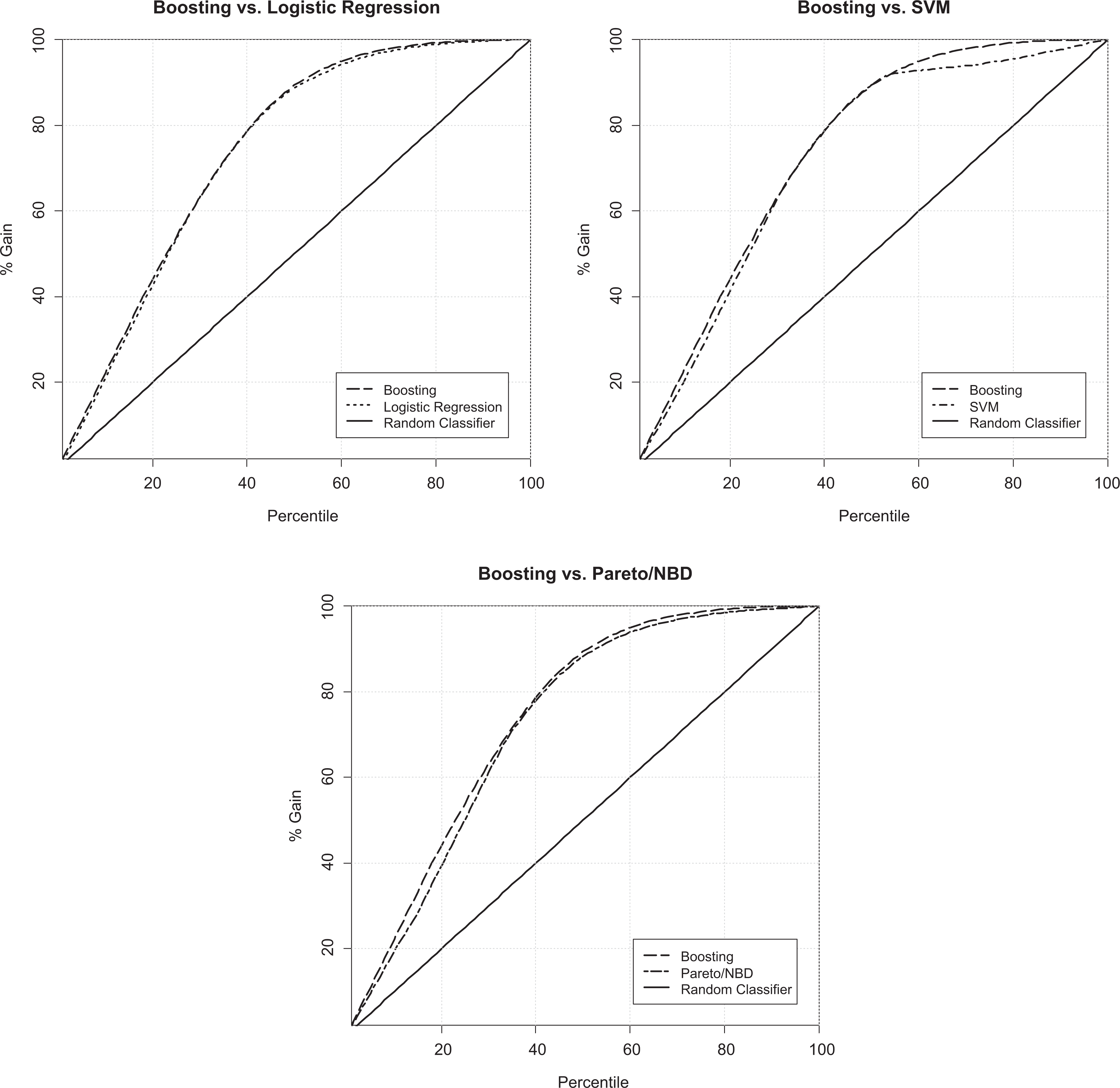
Cumulative lift charts of classification methods for Phase 1 analysis while predictors restricted to recency- and frequency-based variables (Organization A).

Figure 2.

Cumulative lift charts of classification methods for Phase 1 analysis while predictors restricted to recency- and frequency-based variables (Organization B).

Figure 3.

Cumulative lift charts of classification methods for Phase 2 while multiple predictors employed (Organization A).

Table 1.

Gain (%) for 10th Percentile for Different Models, Data Sets, and Phases.

Model	Phase 1		Phase 2
Model	Organization A	Organization B	Organization A
Boosting	23	12	23
Logistic regression	21	11	21
SVM	19	11	21
Pareto/NBD	19	11	—
RFM	—	—	22

Note. SVM = support vector machine; RFM = recency, frequency, and monetary; NBD = negative binomial distribution.

Several important findings follow from our analysis. We group them into three groups based on the effects of (1) predictive technique, (2) data sets, and (3) number of predictors.

Predictive techniques: One of the striking results is that regardless of the number of predictors (Phases 1 and 2) and regardless of data set (A or B), the boosting model outperforms other models, especially for the top two deciles. Another interesting finding common across both phases is the consistently strong performance of logistic regression. Additionally, the cumulative lift charts extracted for the models in the second phase of the study (Figure 3 and Table 1) also reveal that the RFM model, as a common managerial metric (Gupta et al. 2006; Kumar and Reinartz 2012) also performs satisfactorily in churn (inactivity) prediction (Wübben and Wangenheim 2008).

Data sets: Comparing Figures 1 and 2 shows that regardless of predictive techniques, churn prediction is much more accurate for Organization A than Organization B. This difference can only be attributed to the data peculiarities: Data Set B has smaller sample size, lower number of transactions per customer, and lower spending per transaction than Data Set A. In order to identify what data characteristics contribute to model performance, we will conduct a simulation study later. This will allow us to generalize findings.

Predictors: One would expect that adding more predictors will considerably increase predictive validity of the model. However, as Figures 1 and 3 together with Table 1 show, the differences between results from Phases 1 and 2 are not that large, confirming the proven predictive ability of simple variables such as recency and frequency.

Overall, the cumulative lift charts on both data sets in Phase 1 (Figures 1 and 2) confirm that the boosting technique, as an ensemble learner method from the data mining stream of churn modeling, delivers a higher lift compared to other tested techniques and especially compared to Pareto/NBD. Likewise, in the second phase of the study, when multiple covariates were added to the models, the cumulative charts as presented in Figure 3 again echo boosting’s superiority. However, boosting’s superiority shrinks when more predictors are added. Furthermore, cumulative lift charts in Figure 3 confirm that the simple RFM model performs relatively well against other fairly complex models. Results also suggest that apart from recency- and frequency-based variables, some other variables such as number of failures and loyalty program membership can significantly contribute to building the logit, boosting, and SVM models. Specifically, we confirm previous findings that service failure contributes to churn and loyalty membership decreases likelihood of churn. We have also found evidence that decreases in customers spending on dairy, fresh vegetables, and grocery as well as the decrease in number of items purchased from bakery products, dairy, fresh vegetables, grocery, and meat can be an indicator of churn. However, we could not find any effect of customers’ socioeconomic status on churn. This perhaps can be explained by the variable employed, which in lieu of actual socioeconomic status used suburb as a proxy.

Cumulative Profitability Evaluation

As discussed earlier, cumulative lift has widely been employed to evaluate the performance of churn classifiers by identifying customers with a high propensity to become inactive in the next time period. Nevertheless, one issue that this approach does not take into account is that customers with high likelihoods of becoming inactive are not necessarily customers who can make a purchase with the highest profit in the next period if they are targeted with a retention incentive and remain active for at least one more purchase. Thus, if the company seeks to target would-be churners who can generate the highest profit if they are retained for at least one more transaction, it should rank the customer base based on their expected profit; this is where the metric and approach developed by Lemmens and Gupta (2013) comes into play.

In this regard, as a second measure of the models’ performance, the current study utilizes the maximum profit that a retention campaign can generate for the company using each of the models. With the help of simulation, we assess the effect of developed retention campaigns using different models on extra profit generated by this activity. In this regard, using Equation 1 and for models built in Phases 1 and 2 of the study, the individual-level generated profit for customers in our data sets is calculated when a hypothetical voucher is sent to a customer to encourage him or her to make one purchase in the prediction period. Here, the value of the voucher is assumed to be US$20 and US$4 for customers in Organizations A and B, respectively. The value of the voucher was chosen to be approximately 10% of the average transaction value for all customers in two data sets in calibration period (which is approximately US$200 for Data Set A and US$33 for Data Set B). We assume that the average redemption rates for would-be churners (γ _i ) in a data set equals to 0.3 and for nonchurners (φ _i ) equals to 0.9. However, neither of the redemption rates are the same across customers (i.e., both heterogeneous). Specifically, we allow both rates to have Beta distribution with γ _i ∼ Beta (7.5, 17.5) and φ _i ∼ Beta (9, 1).

Once π _i for all customers is calculated, customers are ranked based on their expected profit (rather than on churn likelihood). We repeat the same computations 1,000 times by drawing another set of redemption rates from Beta distributions and average results over these draws. This allows us not only to eliminate the effect of particular randomly chosen redemption rates but also to incorporate uncertainty in our analysis. By so doing, the cumulative profitability charts of retention campaigns (dashed lines in Figures 4, 5, and 6) for both data sets, based on each of the constructed models and for each phase of the study, can be extracted. The proposed cumulative profitability chart shows what extra profit the company can generate by targeting a certain percentage of customers ranked from most to least attractive from a retention perspective. Moreover, as all these charts have an inverted U shape, it is straightforward to determine the optimum target size and the maximum (predicted) profit of each retention campaign. Also, we can compare predicted profit with actual profit as we know the actual status of customer in prediction period. Let y_i = 1 if customer i is a real churner (the customer remains inactive in the next period if he or she is not approached with an incentive), and y_i = 0 if customer i is a real nonchurner (customer purchases in next period). The real profit can be calculated using Equation 4, and its cumulative charts can be similarly extracted using Equation 1 (continuous black lines in Figures 4, 5, and 6). We also can derive precisely the value of V_iP , which is based on profits from previous transactions. Knowing the dollar amount of each purchase and composition of the basket together with margins for each category, we can derive the exact profit that company received from each transaction (see Equations 2 to 4).

Figure 4.

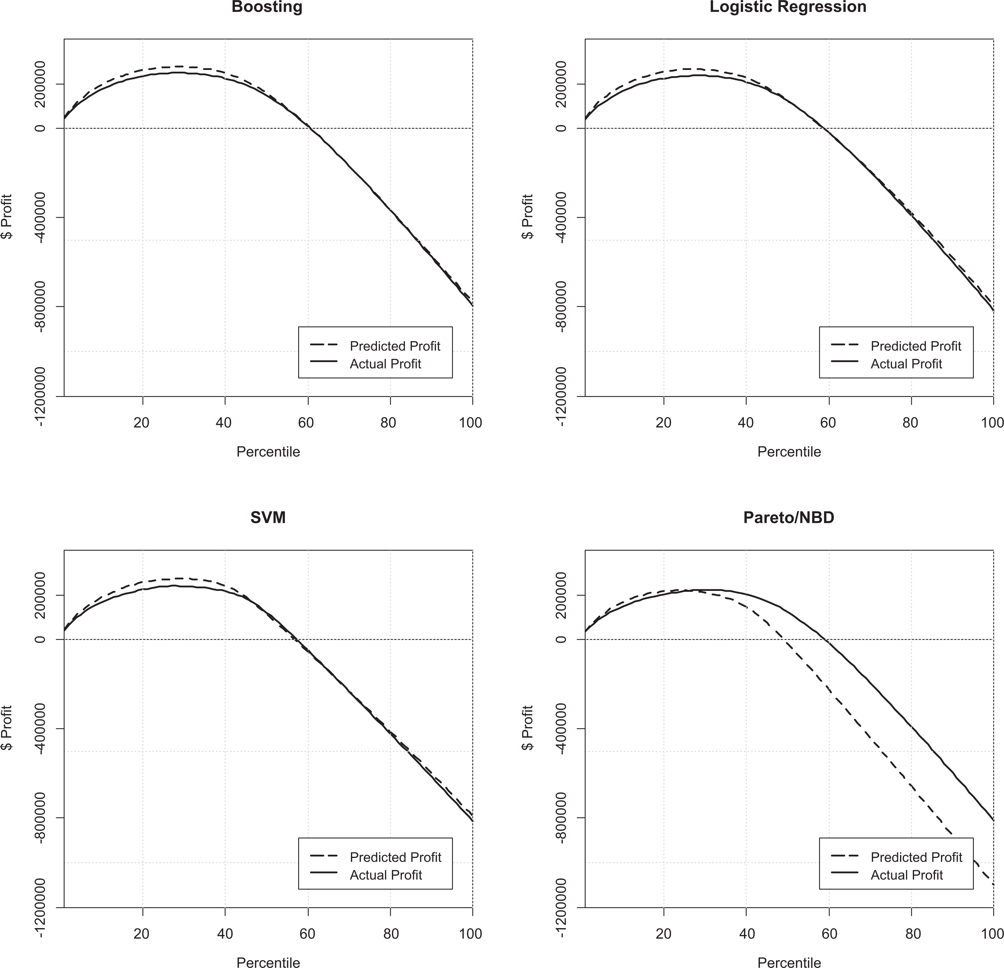
Predicted versus actual profit of the retention campaigns for Organization A (Phase 1 of analysis: predictors are restricted to recency- and frequency-based variables).

Figure 5.

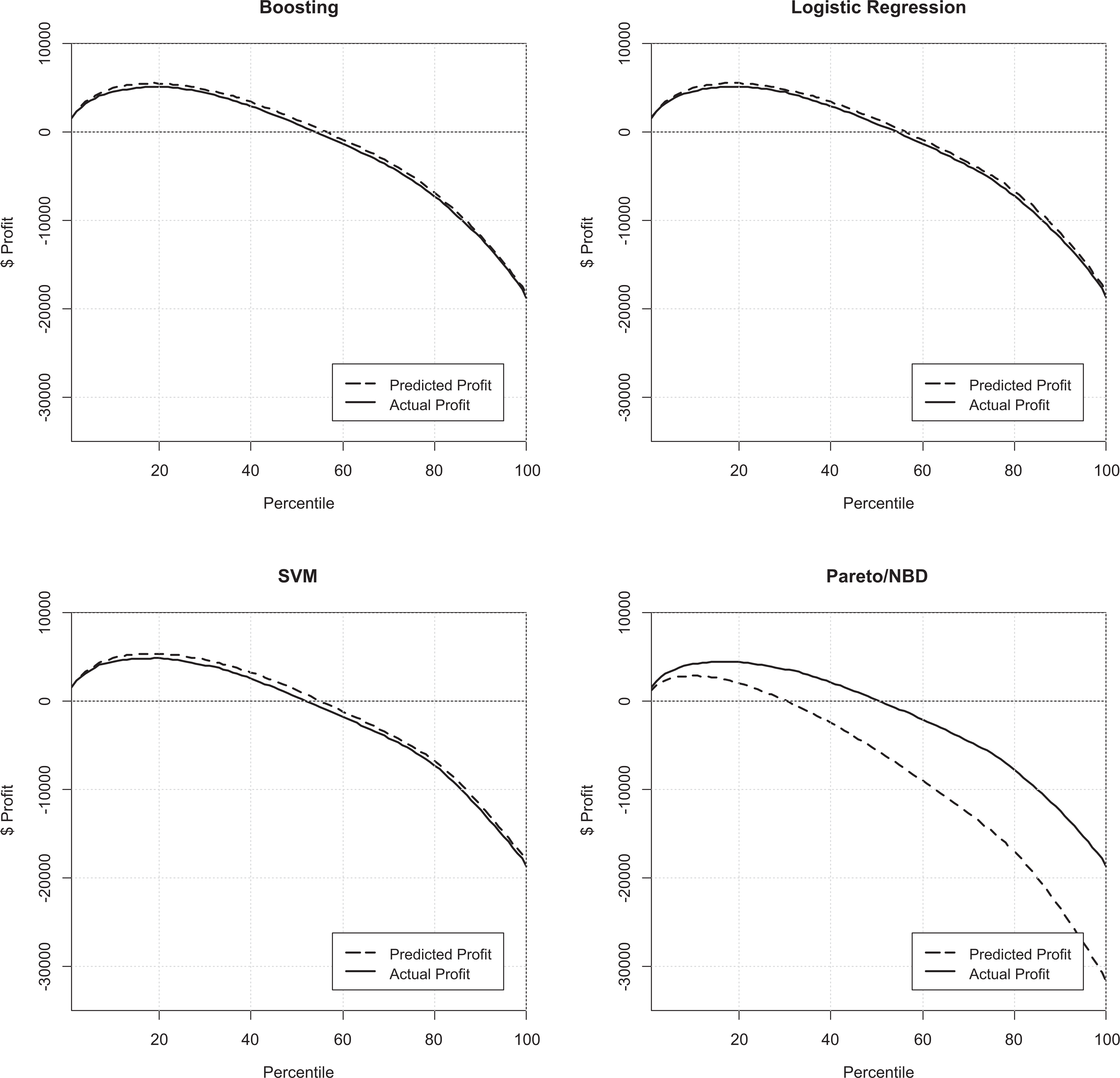
Predicted versus actual profit of the retention campaigns for Organization B (Phase 1 of analysis: predictors are restricted to recency- and frequency-based variables).

Figure 6.

Predicted versus actual profit of the retention campaigns (Phase 2 of analysis: multiple predictors are employed).

π_{real (i)} = {\begin{matrix} γ_{i} (V_{i P} - δ), if y_{i} = 1 \\ - φ_{i} δ, if y_{i} = 0 \end{matrix} .

As we had data for both calibration and prediction periods, we could produce both predicted and actual profits of the retention campaigns. However, in a real-life scenario, managers only have past data. Fortunately, predicted and actual profits are quite close and the maximum predicted profit is very close to the maximum actual profit. Therefore, using the proposed approach, managers can make their decisions based on predicted figures and be confident that the realization will be close to prediction. These maximum profits are presented in Table 2.

Table 2.

Maximum Actual Profit (US$) for Different Models, Data Sets, and Phases.

Model	Phase 1		Phase 2
Model	Organization A	Organization B	Organization A
Boosting	249,083 (241,795; 255,873)	5,088 (4,934; 5,232)	253,410 (246,141; 260,171)
Logistic regression	236,955 (230,155; 243,282)	5,138 (4,980; 5,286)	240,650 (233,700; 247,120)
SVM	240,262 (232,962; 247,082)	4,821 (4,664; 4,967)	245,430 (238,163; 252,206)
Pareto/NBD	215,211 (208,617; 221,375)	4,200 (4,076; 4,316)	—
RFM	—	—	227,543 (220,503; 234,127)

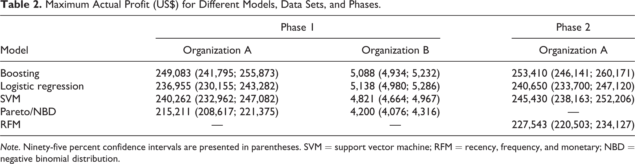
Note. Ninety-five percent confidence intervals are presented in parentheses. SVM = support vector machine; RFM = recency, frequency, and monetary; NBD = negative binomial distribution.

It is important to mention that targeting potential churners is quite a risky endeavor, but if well executed, can be lucrative. Figures 4 to 6 confirm that mass targeting without careful selection can be ruinous. For instance, targeting more than 50% of the customer base can generate negative profits for retention campaigns with losses accumulating rapidly into hundreds of thousands of dollars. The reason for this is that customers who were not planning to defect or be inactive receive vouchers, invariably redeem them, but do not change their behavior, meaning the company wasted money on ineffective retention actions.

In terms of optimization, the highest actual profit of a retention campaign in both phases of the study for Organization A is achieved when the campaign is designed using the boosting model (US$249,083 and US$253,410, respectively). The difference is not statistically significant¹ though, indicating that extra variables did not improve prediction much. However, boosting produced significant differences over other techniques. For Organization B, logistic regression outperformed boosting, but the difference is not statistically significant. Surprisingly, among all four retention campaigns designed based on the classifiers in Phase 1 of the study, the lowest profit is generated by Pareto/NBD, thereby questioning its applicability.

It is also important to note that all figures presented in Table 2 are calculated under the assumption that would-be churners become inactive after making one extra purchase. This is a very conservative assumption, but we make it purposefully. Needless to say, if customers stay active for a longer period (more transactions), the extra profit generated by this retention practice would become even higher.

Overall, based on cumulative lift and profit measures extracted from both data sets and in both phases of the study, the boosting model as an ensemble learner from data mining stream of churn modeling outperforms all other tested models. Specifically, in the first phase of the study, the boosting technique clearly outperforms the Pareto/NBD model. Results also point to the inferiority of Pareto/NBD against the other tested models, in line with Wübben and Wangenheim (2008). Our findings can improve the accuracy of the CLV framework proposed by Reinartz and Kumar (2003), where P(Alive) extracted from the Pareto/NBD model is replaced by a churn score extracted from a boosting model. Furthermore, the analysis of models in the second phase of the study confirms our earlier argument on the importance of using different evaluative criteria to judge the performance of the models. For instance, according to Table 1, the boosting model only marginally outperforms the RFM model from a cumulative lift perspective. However, comparing the performance of the two models in Table 2, based on the profit they can produce when implementing retention campaigns (as we proposed in this study), one finds a significant difference in model performance (US$253,410 vs. US$227,543).

Sensitivity analysis

We have implemented heterogeneous redemption rates across customer base for profit calculation, which allowed us to capture uncertainty. However, it is not clear whether the distribution of redemption rates itself plays an important role. Therefore, we conduct additional sensitivity analysis, by fixing the mean of the distribution for redemption rate (γ) and vary the degree of variability among customers. Thus, we evaluate the maximum profit for boosting technique for Organization A in Phase 2 depending on the variance of redemption rate across customers. The alternative distributions of γ and maximum profits from campaigns are presented in Table 3 (first four rows). Interestingly, regardless of the variance of γ, profits remain almost the same when means are fixed (differences are not significant). We therefore conclude that the spread of the distribution for redemption rates does not play an impactful role in determining maximum profit. However, if we fix variance and vary mean (last two rows in Table 3), the change in profit is highly significant. Therefore, the most important factor is the average of redemption rates in the customer base and not the degree of their variability.

Table 3.

Maximum Actual Profit (US$) for Different Distributions of Redemption Rate γ.

Distribution of γ	Mean (γ)	ln [var(γ)]	Profit
γ ∼ Beta (7.5, 17.5)	0.3	−4.819	253,410 (246,141; 260,171)
γ ∼ Beta (34.5, 80.5)	0.3	−6.314	246,365 (242,722; 249,516)
γ ∼ Beta (148.5, 346.5)	0.3	−7.767	247,495 (245,444; 249,051)
γ ∼ Beta (640.5, 1,494.5)	0.3	−9.227	246,690 (245,320, 247,567)
γ ∼ Beta (3.76, 15.05)	0.2	−4.819	136,785 (130,476; 142,820)
γ ∼ Beta (11.48, 17.23)	0.4	−4.819	375,270 (367,616; 382,175)

Simulation

Our results so far show that boosting model outperforms other techniques based not only on cumulative lift but also on profitability measures. Online Appendix D details the factors to which this superiority can be attributed. Although results were consistent for two data sets, it is important to provide more evidence in order to derive empirical generalizations (Bass and Wind 1995). Simulations are designed in such way that data characteristics of interest are manipulated and, therefore, their effects can be established and measured. The advantage of simulation is that data can be controlled to a higher degree than analyzing multiple real data sets. However, the drawback of simulations is that certain data generating process should be chosen to generate synthetic data. This could be problematic in our case, as we aim to find out which methods best predict churn, and if certain methods are used for data generation, the same method(s) will perform best for prediction. Fortunately, there is a simple and elegant solution to this problem. Instead of generating fully synthetic data, new data can be created from existing empirical data (Burez and Van den Poel 2009). This can be achieved by randomly drawing observations from real data but at the same time controlling certain properties. The relevant properties for our study are (a) sample size, (b) frequency of purchases, and (c) ratio of churners.

Therefore, a random sample of 50,000 customers is selected from Organization A’s data set, as our base sample from which all other subsamples will be created using random sampling and over-/undersampling methods (Burez and Van den Poel 2009). We create (a) 50 samples with different sizes from 500 to 50,000; (b) 25 samples with different average purchase frequency per customer from 2 to 26; and (c) 50 samples with different churn ratios from 1% to 100%. We then evaluate boosting, logistic regression, and Pareto/NBD models from Phase 1 of the study on created samples and compute top decile lifts. Figures 7 to 9 illustrate how changing the three main characterizes of a data set can influence the performance of models in terms of their top decile lift for churn prediction.

Figure 7.

Performance of boosting, logistics regression, and Pareto/NBD models based on top decile lift measure and data sets with different sizes.

Figure 8.

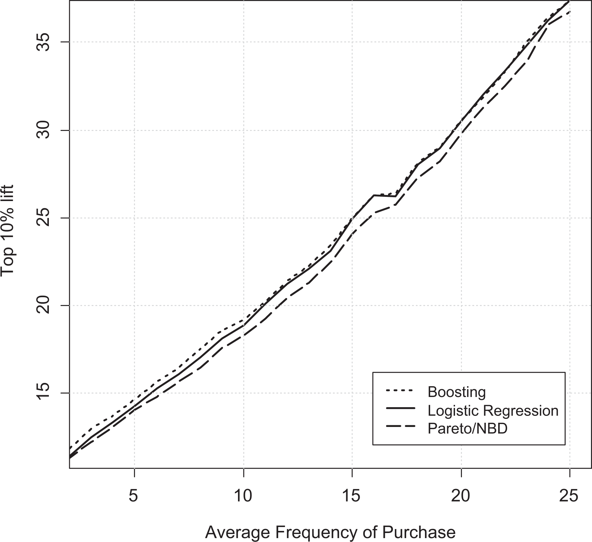
Performance of boosting, logistics regression, and Pareto/NBD models based on top decile lift measure and for data sets with different average frequency of purchase.

Figure 9.

Performance of boosting, logistics regression, and Pareto/NBD models based on top decile lift measure and for data sets with different churn ratios.

Sample Size

Figure 7 shows that for very small sample sizes, the Pareto/NBD model has the upper hand. However, across other (larger) sample sizes, boosting proves to be the best performing model. Another finding is that the performance of models to predict churn is not sensitive to sample sizes. Therefore, for data sets with more than 1,000 observations, adding more data points will not increase predictive performance significantly.

Frequency of Purchases

Figure 8 shows that higher average frequency of purchase leads to better performance of all evaluated models in predicting churn, but boosting consistently outperforms other models across almost the entire range of frequencies. For high levels of purchase frequencies, logistic regression performs as well as boosting.

Churn Ratio

Finally, Figure 9 illustrates that churn ratio is negatively associated with top decile lift. This can be explained by the fact that with more churners, the random model will perform better and better and it becomes more and more difficult for other models to improve on it. For samples with very small churn ratios (up to 4%), logistics regression performs the best, followed by Pareto/NBD. However, as churn ratio increases, the boosting technique starts to outperform all models, while Pareto/NBD remains the least favorable. Finally, for data sets with high churn ratios, the difference between models becomes negligible and they converge to the same performance.

Based on our findings, we offer a guide (Table 4) as to which technique to adopt for predicting churn—based on different data properties. For a wide range of sample sizes (from small to very large samples), boosting outperforms other models and it is only for very small samples that Pareto/NBD model is favored. When the frequency of purchase is low, boosting can deliver the best predictive performance. For medium and above purchase frequencies, both boosting and logistic regression models can be employed, although the logistic regression model might be the preferred due to its ease of implementation. Lastly, for data sets where churn is a very rare event, logistic regression is potentially the best option. As the churn ratio increases, the boosting model begins to catch up. When the churn ratio reaches the “very high” level, all models become almost identical. One should note that the simulation results presented here are obtained in the absence of common balancing techniques to handle class imbalance (Burez and Van den Poel 2009).

Table 4.

A Guide on Using Different Churn Classifiers Based on the Identified Characteristics of a Data Set.

	Very Low/Small	Low/Small	Medium	High/Large	Very High/Large
Sample size	PNBD	BOOST	BOOST	BOOST	BOOST
Average purchase frequency	BOOST	BOOST	LR, BOOST	LR, BOOST	LR, BOOST
Churn ratio	LR	BOOST	BOOST	LR, BOOST, PNBD	LR, BOOST, PNBD

Note. BOOST = boosting; NBD = negative binomial distribution; PNBD = Pareto/NBD; LR = logistic regression.

Discussion and Conclusions

Summary of Findings

Many studies have espoused the merits of data mining and probability modeling (Hopmann and Thede 2005; Neslin et al. 2006; Wübben 2008; Wübben and Wangenheim 2008) in predicting customer churn. Nevertheless, to the best of our knowledge, the current study is among the first to (1) simultaneously investigate the performance of (two) data mining predictive models, a probability model, logistic regression, and the RFM metric in predicting customer churn in noncontractual settings; (2) evaluate and compare the performance of different customer churn classifiers by operationalizing a novel profit metric which is based on the expected incremental profit of each customer when he or she is targeted with a retention incentive while accounting for customers’ heterogeneity; and (3) provide managerial recommendations as to which techniques to use under what circumstances.

In this regard, we have benchmarked two data mining techniques (SVM as a single algorithm technique and boosting as an ensemble learner) and one probability model (Pareto/NBD) against logistic regression and the RFM model in terms of their performance from a cumulative lift perspective. We have also performed analysis with both limited (Phase 1: online grocery retailer and online CD retailer) and extended number of predictors (Phase 2: online grocery retailer). Our analysis in two phases of the study and on data sets from two different contexts confirms the relative superiority of the boosting technique based on the cumulative lift when compared with Pareto/NBD, SVM, logistic regression, and RFM. This also enables us to propose a superior alternative to the Pareto/NBD model used by Reinartz and Kumar (2003) in developing their CLV framework.

In addition, in order to compare the models in terms of the profit they can produce in a customer retention sense, we evaluate their performance in a simulated churn management campaign. We assume that the firm aims to provide customers who are likely to become inactive in the next period, with an incentive in the form of a voucher to persuade them to make at least one purchase in the next time period. Our findings suggest that campaigns designed using the boosting technique can generate the highest profit for the company when compared with campaigns designed using SVM, logistic regression, Pareto/NBD, or RFM methods. Moreover, campaigns designed using Pareto/NBD generate the lowest profit. Furthermore, our results suggest that the Pareto/NBD model, as one of the most popular models from the probability modeling stream, is unable to outperform logistic regression—a traditional approach used by marketing academics and practitioners.

Lastly, our analysis on simulated data where primary characteristics of a data set (i.e., sample size, average frequency of purchase, and churn ratio) are manipulated, once again confirming the superiority of the boosting model under most conditions. The only exceptions are when the churn ratio is very low (where logistic regression excels) and when the data set is small (where Pareto/NBD prevails).

Managerial Implications

Companies that rely on a proactive targeted approach (Burez and Van den Poel 2007) in dealing with churn are interested in identifying customers at “defection risk.” However, not all would-be churners are profitable if retained. Thus, in reality, companies are interested in identifying those who are at churn risk and expected to be profitable if targeted with a retention incentive. This information would enable companies to target such customers with tailored incentives to persuade them to stay. Such strategies have the benefit of lower costs as incentives are expected to be lower than in the case of customers who have already left the company and have to be “bribed” to return. The implementation of a proactive targeted strategy in dealing with customer churn calls for accurate prediction models, the identification of which has been an objective of this study.

Our findings are particularly useful to managers looking to improve marketing ROI by accurately identifying customers more likely to defect and carefully targeting those with more profit potential to make at least one additional purchase. More importantly, the study provides managers (especially in the online retail and similar contexts) with a guide to help select the appropriate method based on their specific data set characteristics. Accordingly, the findings suggest that in order for companies to establish an effective churn management regime, a “toolbox” of modeling techniques is required. This would enable managers to decide on the most powerful technique depending on context of the business, size of the business, and behavior of customers. In particular, our findings suggest that where the size of the customer base is very small (e.g., local organic food store), Pareto/NBD can best capture churn intention. However, for companies with large customer bases such as online retailers with thousands of customers, data mining techniques and specifically the boosting technique can deliver better predictive power. In addition, practitioners are advised to consider the purchasing patterns of customers while choosing the modeling approach. As the simulation study shows, for a great range of companies, including those with a very low (e.g., vacuum cleaner retailer) to medium (e.g., an online fashion retailer) purchase frequencies, the boosting technique delivers the most promising prediction accuracy. However, it is expected that for businesses such as grocery retailers where the frequency of purchases is high, logistic regression, as parametric technique, rivals boosting. Also, in cases/contexts where churn is a very rare event, logistics regression is expected to deliver superior predictive power. Nevertheless, as the churn ratio increases, boosting begins to prevail. For companies with very high churn ratios, since all three tested models appear to deliver the same predictive power, logistic regression can be the best choice for managers due to its transparency, interpretability, and ease of use. It should be noted that since high/low churn ratio is not necessarily specific to a particular context, managers are advised to closely observe the dynamics of churn ratio within company’s customer base over time and employ the appropriate modeling approach accordingly.

Limitations and Further Research

Simulations have enabled us to detect certain patterns of model performance under different circumstances—allowing us to empirically generalize our findings beyond the specifics of our data sets and establish a more generalizable rule in terms of “which methodology is more appropriate when?” Although our simulation results have validity in online retailing, we acknowledge that they may not necessarily hold in other significantly different contexts.

The unavailability of more service-related variables in our data sets has hindered our ability to explore how factors such as service quality and customer satisfaction impact the predictive quality of our churn models. However, this provides rich avenues for future studies to investigate such effects using data sets containing more service-related variables. The absence of robust promotion data required us to perform simulations on profitability analysis. Using real data on voucher distribution could be another interesting direction for further research. A recent study (Kumar, Bhagwat, and Xi 2015) investigated the effect of offer content on probability of customer win back. Testing the effect of the offer content in customer retention is another direction for future research. Finally, the model can be extended to incorporate the potential link between the value of promotion incentive and the probability of accepting the offer into the profitability metric.

Footnotes

Declaration of Conflicting Interests

The author(s) declared no potential conflicts of interest with respect to the research, authorship, and/or publication of this article.

Funding

The author(s) received no financial support for the research, authorship, and/or publication of this article.

Note

Supplemental Material

The online appendices are available at

References

Alpaydin

Ethem

(1999), “Combined 5 × 2 cv F Test for Comparing Supervised Classification Learning Algorithms,” Neural Computation, 11 (8), 1885–1892.

Athanassopoulos

Antreas D.

(2000), “Customer Satisfaction Cues to Support Market Segmentation and Explain Switching Behavior,” Journal of Business Research, 47 (3), 191–207.

Bass

Frank M.

Wind

Jerry

(1995), “Introduction to the Special Issue: Empirical Generalizations in Marketing,” Marketing Science, 14 (3), G1–G5.

Bijmolt

Tammo H. A.

Leeflang

Peter S. H.

Block

Frank

Eisenbeiss

Maik

Hardie

Bruce

Lemmens

Aurélie

Saffert

Peter

(2010), “Analytics for Customer Engagement,” Journal of Service Research, 13 (3), 341–356.

Boser

Bernhard E.

Guyon

Isabelle M.

Vapnik

Vladimir N.

(1992), “A Training Algorithm for Optimal Margin Classifiers,” in Proceedings of the Fifth Annual Workshop on Computational Learning Theory, David

Haussler

, ed. Pittsburgh, PA: ACM, 144–152.

Breiman

Leo

(1996), “Bagging Predictors,” Machine Learning, 24 (2), 123–140.

Buckinx

Wouter

Poel

Dirk Van den

(2005), “Customer Base Analysis: Partial Defection of Behaviourally Loyal Clients in a Non-contractual FMCG Retail Setting,” European Journal of Operational Research, 164 (1), 252–268.

Burez

Jonathan

Poel

Dirk Van den

(2009), “Handling Class Imbalance in Customer Churn Prediction,” Expert Systems with Applications, 36 (3), 4626–4636.

Burez

Jonathan

Poel

Dirk Van den

(2007), “CRM at a Pay-TV Company: Using Analytical Models to Reduce Customer Attrition by Targeted Marketing for Subscription Services,” Expert Systems with Applications, 32 (2), 277–288.

10.

Coussement

Kristof

De Bock

Koen W.

(2013), “Customer Churn Prediction in the Online Gambling Industry: The Beneficial Effect of Ensemble Learning,” Journal of Business Research, 66 (9), 1629–1636.

11.

Coussement

Kristof

Poel

Dirk Van den

(2009), “Improving Customer Attrition Prediction by Integrating Emotions from Client/Company Interaction Emails and Evaluating Multiple Classifiers,” Expert Systems with Applications, 36 (3, Part 2), 6127–6134.

12.

Cui

Dapeng

Curry

David

(2005), “Prediction in Marketing Using the Support Vector Machine,” Marketing Science, 24 (4), 595–615.

13.

Bock

Koen

Poel

Dirk Van den

(2011), “An Empirical Evaluation of Rotation-based Ensemble Classifiers for Customer Churn Prediction,” Expert Systems with Applications, 38 (10), 12293–12301.

14.

Ehrenberg

Andrew S. C.

(1959), “The Pattern of Consumer Purchases,” Journal of the Royal Statistical Society, 8 (1), 26–41.

15.

Fader

Peter S.

Hardie

Bruce

(2009), “Probability Models for Customer-base Analysis,” Journal of Interactive Marketing, 23 (1), 61–69.

16.

Fader

Peter S.

Hardie

Bruce

(2001), “Forecasting Repeat Sales at CDNOW: A Case Study,” Interfaces, 31 (3), S94–S107.

17.

Fader

Peter S.

Hardie

Bruce

Lok Lee

(2005), “Counting Your Customers” the Easy Way: An Alternative to the Pareto/NBD Model,” Marketing Science, 24 (2), 275–284.

18.

Forbes (2011), “Bringing 20/20 Foresight to Marketing: CMOs Seek a Clearer Picture of the Customer,” Forbes Insights, 1–13.

19.

Fruchter

Gila E.

John Zhang

(2004), “Dynamic Targeted Promotions: A Customer Retention and Acquisition Perspective,” Journal of Service Research, 7 (1), 3–19.

20.

Gupta

Sunil

Hanssens

Dominique

Hardie

Bruce

Kahn

William

Kumar

Lin

Nathaniel

Ravishanker

nalini

Sriram

(2006), “Modeling Customer Lifetime Value,” Journal of Service Research, 9 (2), 139–155.

21.

Han

Jiawei

Kamber

Micheline

Pei

Jian

(2011), Data Mining: Concepts and Techniques, 3rd ed. San Francisco, CA: Morgan Kaufmann.

22.

Homburg

Christian

Giering

Christian Annette

(2001), “Personal Characteristics as Moderators of the Relationship between Customer Satisfaction and Loyalty: An Empirical Analysis,” Psychology & Marketing, 18 (1), 43–66.

23.

Hopmann

Jörg

Thede

Anke

(2005), “Applicability of Customer Churn Forecasts in a Non-Contractual Setting,” in Innovations in Classification, Data Science, and Information Systems (Proceedings of the 27th Annual Conference of the Gesellschaft für Klassifikation e.V., Brandenburg University of Technology, Cottbus, March 12–14, 2003), Daniel

Baier

Klaus-Dieter

Wernecke

, eds. Berlin, Germany: Springer-Verlag, 330–337.

24.

Hoppe

Daniel

Wagner

Uno

(2007), “Customer Base Analysis: The Case for a Central Variant of the Betageometric/NBD Model,” Marketing: Journal of Research and Management, 3 (2), 75–90.

25.

Huang

Bingquan

Kechadi

Mohand T.

Buckley

Brian

(2012), “Customer Churn Prediction in Telecommunications,” Expert Systems with Applications, 39 (1), 1414–1425.

26.

Kamakura

Wagner

Mela

Carl

Ansari

Asim

Bodapati

Anand

Fader

Pete

Iyengar

Raghuram

Naik

Prasad

Sun

Scott Neslin Baohong

Verhoef

Peter

Wedel

Michel

Wilcox

Ron

(2005), “Choice Models and Customer Relationship Management,” Marketing Letters, 16 (3), 279–291.

27.

Keaveney

Susan M.

(1995), “Customer Switching Behavior in Service Industries: An Exploratory Study,” Journal of Marketing, 59 (2), 71–82.

28.

Keiningham

Timothy L.

Morgeson

Forest V.

Aksoy

Lerzan

Williams

Luke

(2014), “Service Failure Severity, Customer Satisfaction, and Market Share: An Examination of the Airline Industry,” Journal of Service Research, 17 (4), 415–431.

29.

Kumar

Bhagwat

Yashoda

Zhang

(2015), “Regaining “Lost” Customers: The Predictive Power of First-Lifetime Behavior, the Reason for Defection, and the Nature of the Win-Back Offer,” Journal of Marketing, 79 (4), 34–55.

30.

Kumar

Reinartz

Werner

(2012), Customer Relationship Management: Concept, Strategy, and Tools. Berlin, Germany: Springer

31.

Lemmens

Aurélie

Christophe Croux

(2006), “Bagging and Boosting Classification Trees to Predict Churn,” Journal of Marketing Research, 43 (2), 276–286.

32.

Lemmens

Aurélie

Gupta

Sunil

(2013), “Managing Churn to Maximize Profits,” Working Paper, Harvard Business School, Boston, MA.

33.

Meyer-Waarden

Lars

(2008), “The Influence of Loyalty Programme Membership on Customer Purchase Behaviour,” European Journal of Marketing, 42 (1/2), 87–114.

34.

Miguéis

V. L.

Camanho

Ana

Cunha

João Falcão e

(2013), “Customer Attrition in Retailing: An Application of Multivariate Adaptive Regression Splines,” Expert Systems with Applications, 40 (16), 6225–6232.

35.

Neslin

Scott A.

Gupta

Sunil

Kamakura

Wagner

Junxiang

Mason

Charlotte H.

(2006), “Defection Detection: Measuring and Understanding the Predictive Accuracy of Customer Churn Models,” Journal of Marketing Research, 43 (2), 204–211.

36.

Reinartz

Werner J.

Kumar

(2003), “The Impact of Customer Relationship Characteristics on Profitable Lifetime Duration,” Journal of Marketing, 67 (1), 77–99.

37.

Reinartz

Werner J.

Kumar

(2000), “On the Profitability of Long-Life Customers in a Noncontractual Setting: An Empirical Investigation and Implications for Marketing,” Journal of Marketing, 64 (4), 17–35.

38.

Risselada

Hans

Verhoef

Peter C.

Bijmolt

Tammo H. A.

(2010), “Staying Power of Churn Prediction Models,” Journal of Interactive Marketing, 24 (3), 198–208.

39.

Roos

Inger

Gustafsson

Anders

(2007), “Understanding Frequent Switching Patterns,” Journal of Service Research, 10 (1), 93–108.

40.

Rust

Ronald T.

Lemon

Katherine N.

Zeithaml

Valarie A.

(2004), “Return on Marketing: Using Customer Equity to Focus Marketing Strategy,” Journal of Marketing, 68 (1), 109–127.

41.

Schmittlein

David C.

Morrison

Donald G.

Colombo

Richard

(1987), “Counting Your Customers: Who Are They and What Will They Do Next?,” Management Science, 33 (1), 1–24.

42.

Sirgy

M. Joseph

Coskun Samli

(1985), “A Path Analytic Model of Store Loyalty Involving Self-Concept, Store Image, Geographic Loyalty, and Socioeconomic Status,” Journal of Academy of Marketing Science, 13 (3), 265–291.

43.

Venkatesan

Rajkumar

Kumar

(2004), “A Customer Lifetime Value Framework for Customer Selection and Resource Allocation Strategy,” Journal of Marketing, 68 (4), 106–125.

44.

Couchen

Chen

hsiu-Li

(2000), “Counting Your Customers: Compounding Customer’s In-Store Decisions, Interpurchase Time and Repurchasing Behavior,” European Journal of Operational Research, 127 (1), 109–119.

45.

Wübben

Markus

(2008), Analytical CRM: Developing and Maintaining Profitable Customer Relationships in Non-contractual Settings. New York, NY: Springer.

46.

Wübben

Markus

Wangenheim

Florian V.

(2008), “Instant Customer Base Analysis: Managerial Heuristics Often “Get it Right”,” Journal of Marketing, 72 (3), 82–93.

47.

Xiaobing

Guo

Shunsheng

Guo

Jun

Huang

Xiaorong

(2011), “An Extended Support Vector Machine Forecasting Framework for Customer Churn in E-Commerce,” Expert Systems with Applications, 38 (3), 1425–1430.

Supplementary Material

Please find the following supplemental material available below.

For Open Access articles published under a Creative Commons License, all supplemental material carries the same license as the article it is associated with.

For non-Open Access articles published, all supplemental material carries a non-exclusive license, and permission requests for re-use of supplemental material or any part of supplemental material shall be sent directly to the copyright owner as specified in the copyright notice associated with the article.

0.00 MB

0.17 MB

0.85 MB